Unsupervised Progressive Learning and the STAM Architecture
←
→
Page content transcription
If your browser does not render page correctly, please read the page content below

Unsupervised Progressive Learning and the STAM Architecture

                                                            James Smith∗ , Cameron Taylor∗ , Seth Baer and Constantine Dovrolis†
                                                                                  1
                                                                                    Georgia Institute of Technology
                                                            { jamessealesmith, cameron.taylor, cooperbaer.seth, constantine}@gatech.edu,
arXiv:1904.02021v6 [cs.LG] 13 May 2021

                                                                      Abstract                                  dimensionality that, ideally, makes it easier to identify the
                                                                                                                explanatory factors of variation behind the data [Bengio et al.,
                                                 We first pose the Unsupervised Progressive Learn-              2013], leading to better performance in tasks such as clustering
                                                 ing (UPL) problem: an online representation learn-             or classification. FL methods differ in the prior P (h) and the
                                                 ing problem in which the learner observes a non-               loss function. A similar approach is self-supervised methods,
                                                 stationary and unlabeled data stream, learning a               which learn representations by optimizing an auxiliary task
                                                 growing number of features that persist over time              [Gidaris et al., 2018].
                                                 even though the data is not stored or replayed. To                In this work, we focus on a new and pragmatic problem that
                                                 solve the UPL problem we propose the Self-Taught               adopts some elements of CL and FL but is also different than
                                                 Associative Memory (STAM) architecture. Lay-                   them – we refer to this problem as single-pass unsupervised
                                                 ered hierarchies of STAM modules learn based on a              progressive learning or UPL for short. UPL can be described
                                                 combination of online clustering, novelty detection,           as follows:
                                                 forgetting outliers, and storing only prototypical fea-        (1) The data is observed as a non-IID stream (e.g., different
                                                 tures rather than specific examples. We evaluate               portions of the stream may follow different distributions and
                                                 STAM representations using clustering and classi-              there may be strong temporal correlations between successive
                                                 fication tasks. While there are no existing learning           examples), (2) the features should be learned exclusively from
                                                 scenarios that are directly comparable to UPL, we              unlabeled data, (3) each example is “seen” only once and the
                                                 compare the STAM architecture with two recent con-             unlabeled data are not stored for iterative processing, (4) the
                                                 tinual learning models, Memory Aware Synapses                  number of learned features may need to increase over time, in
                                                 (MAS) and Gradient Episodic Memories (GEM),                    response to new tasks and/or changes in the data distribution,
                                                 after adapting them in the UPL setting. 1                      (5) to avoid catastrophic forgetting, previously learned features
                                                                                                                need to persist over time, even when the corresponding data
                                         1       Introduction                                                   are no longer observed in the stream.
                                         The Continual Learning (CL) problem is predominantly ad-                  The UPL problem is encountered in important AI appli-
                                         dressed in the supervised context with the goal being to learn         cations, such as a robot learning new visual features as it
                                         a sequence of tasks without “catastrophic forgetting” [Good-           explores a time-varying environment. Additionally, we argue
                                         fellow et al., 2013]. There are several CL variations but a            that UPL is closer to how animals learn, at least in the case
                                         common formulation is that the learner observes a set of ex-           of perceptual learning [Goldstone, 1998]. We believe that in
                                         amples {(xi , ti , yi )}, where xi is a feature vector, ti is a task   order to mimic that, ML methods should be able to learn in a
                                         identifier, and yi is the target vector associated with (xi , ti )     streaming manner and in the absence of supervision. Animals
                                         [Lopez-Paz and Ranzato, 2017]. Other CL variations replace             do not “save off" labeled examples to train in parallel with
                                         task identifiers with task boundaries that are either given [Hsu       unlabeled data, they do not know how many “classes” exist
                                         et al., 2018] or inferred [Zeno et al., 2018]. Typically, CL           in their environment, and they do not have to replay/dream
                                         requires that the learner either stores and replays some previ-        periodically all their past experiences to avoid forgetting them.
                                         ously seen examples [Rebuffi et al., 2017] or generates exam-             To address the UPL problem, we describe an architecture
                                         ples of earlier learned tasks [Shin et al., 2017].                     referred to as STAM (“Self-Taught Associative Memory”).
                                            The Unsupervised Feature (or Representation) Learning               STAM learns features through online clustering at a hierarchy
                                         (FL) problem, on the other hand, is unsupervised but mostly            of increasing receptive field sizes. We choose online clustering,
                                         studied in the offline context: given a set of examples {xi },         instead of more complex learning models, because it can be
                                         the goal is to learn a feature vector hi = f (xi ) of a given          performed through a single pass over the data stream. Further,
                                                                                                                despite its simplicity, clustering can generate representations
                                             ∗
                                               These authors contributed equally to this work.                  that enable better classification performance than more com-
                                             †
                                               Contact Author                                                   plex FL methods such as sparse-coding or some deep learning
                                             1
                                               Code available at https://github.com/CameronTaylorFL/stam        methods [Coates et al., 2011]. STAM allows the number of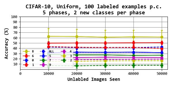
clusters to increase over time, driven by a novelty detection
mechanism. Additionally, STAM includes a brain-inspired
dual-memory hierarchy (short-term versus long-term) that en-
ables the conservation of previously learned features (to avoid
catastrophic forgetting) that have been seen multiple times at
the data stream, while forgetting outliers. To the extent of our
knowledge, the UPL problem has not been addressed before.
The closest prior work is CURL (“Continual Unsupervised
Representation Learning”) [Rao et al., 2019]. CURL however
does not consider the single-pass, online learning requirement.
We further discuss this difference with CURL in Section 7.
2    STAM Architecture
In the following, we describe the STAM architecture as a se-                Figure 1: A hypothetical pool of STM and LTM centroids visualized
                                                                            at seven time instants. From ta to tb , a centroid is moved from STM
quence of its major components: a hierarchy of increasing
                                                                            to LTM after it has been selected θ times. At time tb , unlabeled
receptive fields, online clustering (centroid learning), novelty            examples from classes ‘2’ and ‘3’ first appear, triggering novelty
detection, and a dual-memory hierarchy that stores prototyp-                detection and new centroids are created in STM. These centroids are
ical features rather than specific examples. The notation is                moved into LTM by td . From td to tg , the pool of LTM centroids
summarized for convenience in the Supplementary Material                    remains the same because no new classes are seen. The pool of
(SM)-A.                                                                     STM centroids keeps changing when we receive “outlier” inputs of
I. Hierarchy of increasing receptive fields: An input vector                previously seen classes. Those centroids are later replaced (Least-
xt ∈ Rn (an image in all subsequent examples) is analyzed                   Recently-Used policy) due to the limited capacity of the STM pool.
through a hierarchy of Λ layers. Instead of neurons or hidden-
layer units, each layer consists of STAM units – in its simplest            III. Novelty detection: When an input patch xl,m at layer l
form a STAM unit functions as an online clustering module.                  is significantly different than all centroids at that layer (i.e.,
Each STAM unit processes one ρl ×ρl patch (e.g. 8×8 subvec-                 its distance to the nearest centroid is a statistical outlier), a
tor) of the input at the l’th layer. The patches are overlapping,           new centroid is created in Cl based on xl,m . We refer to this
with a small stride (set to one pixel in our experiments) to                event as Novelty Detection (ND). This function is necessary
accomplish translation invariance (similar to CNNs). The                    so that the architecture can learn novel features when the data
patch dimension ρl increases in higher layers – the idea is                 distribution changes.
that the first layer learns the smallest and most elementary fea-              To do so, we estimate in an online manner the distance
tures while the top layer learns the largest and most complex               distribution between input patches and their nearest centroid
features.                                                                   (separately for each layer). The novelty detection threshold at
II. Centroid Learning: Every patch of each layer is clustered,
in an online manner, to a set of centroids. These time-varying              layer l is denoted by D̂l and it is defined as the 95-th percentile
centroids form the features that the STAM architecture gradu-               (β = 0.95) of this distance distribution.
ally learns at that layer. All STAM units of layer l share the              IV. Dual-memory organization: New centroids are stored
same set of centroids Cl (t) at time t – again for translation              temporarily in a Short-Term Memory (STM) of limited capacity
invariance.2 Given the m’th input patch xl,m at layer l, the                ∆, separately for each layer. Every time a centroid is selected
nearest centroid of Cl selected for xl,m is                                 as the nearest neighbor of an input patch, it is updated based
                                                                            on (2). If an STM centroid cl,j is selected more than θ times,
                     cl.j = arg min d(xl,m , c)                      (1)    it is copied to the Long-Term Memory (LTM) for that layer.
                                 c∈Cl
                                                                            We refer to this event as memory consolidation. The LTM has
where d(xl,m , c) is the Euclidean distance between the patch               (practically) unlimited capacity and a much smaller learning
xl,m and centroid c.3 The selected centroid is updated based                rate (in our experiments the LTM learning rate is set to zero).
on a learning rate parameter α, as follows:                                    This memory organization is inspired by the Complemen-
           cl,j = α xl,m + (1 − α)cl,j ,        0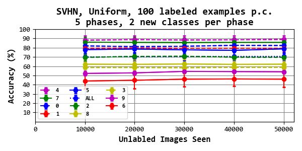
at each layer using randomly sampled patches from the first
few images of the unlabeled stream. The initial value of the
novelty-detection threshold is calculated based on the distance
distribution between each of these initial STM centroids and
its nearest centroid.
3    Clustering using STAM
We can use the STAM features in unsupervised tasks, such as
offline clustering. For each patch of input x, we compute the
nearest LTM centroid. The set of all such centroids, across
all patches of x, is denoted by Φ(x). Given two inputs x and
y, their pairwise distance is the Jaccard distance of Φ(x) and
Φ(y). Then, given a set of inputs that need to be clustered,
and a target number of clusters, we apply a spectral clustering       Figure 2: An example of the classification process. Every patch (at
algorithm on the pairwise distances between the set of inputs.        any layer) that selects a CIN centroid votes for the single class that has
We could also use other clustering algorithms, as long as they        the highest association with. These patch votes are first averaged at
do not require Euclidean distances.                                   each layer. The final inference is the class with the highest cumulative
                                                                      vote across all layers.
4    Classification using STAM
Given a small amount of labeled data, STAM representations            where 1/|L(t)| is the chance term and γ is the significance
can also be evaluated with classification tasks. We emphasize         term.
that the labeled data is not used for representation learning –       III. Classification using a hierarchy of centroids: At test
it is only used to associate previously learned features with a       time, we are given an input x of class k(x) and infer its class
given set of classes.                                                 as k̂(x). The classification task is a “biased voting” process in
I. Associating centroids with classes: Suppose we are given           which every patch of x, at any layer, votes for a single class as
some labeled examples XL (t) from a set of classes L(t) at            long as that patch selects a CIN centroid.
time t. We can use these labeled examples to associate existing          Specifically, if a patch xl,m of layer l selects a CIN centroid
LTM centroids at time t (learned strictly from unlabeled data)        c, then that patch votes vl,m = maxk∈L(t) gc (k) for the class
with the set of classes in L(t).                                      k that has the highest association with c, and zero for all other
    Given a labeled example of class k, suppose that there is         classes. If c is not a CIN centroid, the vote of that patch is
a patch x in that example for which the nearest centroid is           zero for all classes.
c. That patch contributes the following association between              The vote of layer l for class k is the average vote across all
centroid c and class k:                                               patches in layer l (as illustrated in Figure 2):
                     fx,c (k) = e−d(x,c)/D̄l                   (3)                                   P
                                                                                                                vl,m
                                                                                            vl (k) = m∈Ml                            (6)
where D̄l is a normalization constant (calculated as the average                                          |Ml |
distance between input patches and centroids). The class-
association vector gc between centroid c and any class k is           where Ml is the set of patches in layer l. The final inference
computed aggregating all such associations, across all labeled        for input x is the class with the highest cumulative vote across
examples in XL :                                                      all layers:
                   P                                                                                       XΛ
                      x∈XL (k) fx,c (k)                                                  k̂(x) = arg max        vl (k)             (7)
  gc (k) = P            P                   0
                                               , k = 1 . . . L(t)                                        0 k
                          x∈XL (k0 ) fx,c (k )
                                                                                                                l=1
               k0 ∈L(t)
                                                                (4)
where XLP  (k) refers to labeled examples belonging to class k.       5    Evaluation
Note that k gc (k)=1.
                                                                      To evaluate the STAM architecture in the UPL context, we
II. Class informative centroids: If a centroid is associated
                                                                      consider a data stream in which small groups of classes appear
with only one class k (gc (k) = 1), only labeled examples
                                                                      in successive phases, referred to as Incremental UPL. New
of that class select that centroid. At the other extreme, if a
                                                                      classes are introduced two at a time in each phase, and they are
centroid is equally likely to be selected by examples of any
                                                                      only seen in that phase. STAM must be able to both recognize
labeled class, (gc (k) ≈ 1/|L(t)|), the selection of that centroid
                                                                      new classes when they are first seen in the stream, and to also
does not provide any significant information for the class of
                                                                      remember all previously learned classes without catastrophic
the corresponding input. We identify the centroids that are
                                                                      forgetting. Another evaluation scenario is Uniform UPL,
Class INformative (CIN) as those that are associated with at
                                                                      where all classes appear with equal probability throughout the
least one class significantly more than expected by chance.
                                                                      stream – the results for Uniform UPL are shown in SM-G.
Specifically, a centroid c is CIN if
                                                                         We include results on four datasets: MNIST [Lecun et
                                      1                               al., 1998] , EMNIST (balanced split with 47 classes) [Cohen
                   max gc (k) >            +γ                  (5)    et al., 2017] , SVHN [Netzer et al., 2011] , and CIFAR-10
                  k∈L(t)            |L(t)|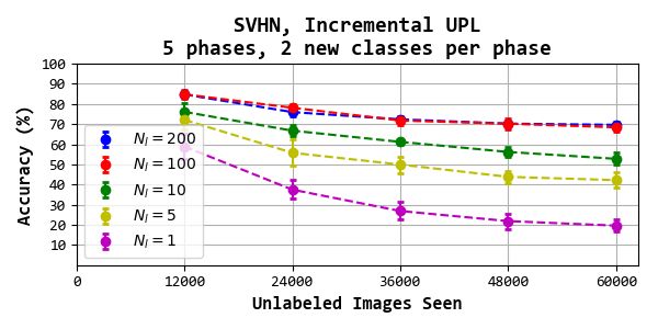
Figure 3: Clustering accuracy for MNIST (left), SVHN (left-center), CIFAR-10 (right-center), and EMNIST (right). The task is expanding
clustering for incremental UPL. The number of clusters is equal to 2 times the number of classes in the data stream seen up to that point in time.

[Krizhevsky et al., 2014] . For each dataset we utilize the                phases in the data stream. This makes the comparison with
standard training and test splits. We preprocess the images by             STAM somehow unfair, because STAM does not have access
applying per-patch normalization (instead of image normaliza-              to this information. The results show however that STAM per-
tion), and SVHN is converted to grayscale. More information                forms better even without knowing the temporal boundaries
about preprocessing can be found in SM-H.                                  of successive phases.
   We create the training stream by randomly selecting, with                  Memory Aware Synapse (MAS) is another supervised
equal probability, Np data examples from the classes seen dur-             continual learning model that expects known task boundaries
ing each phase. Np is set to 10000, 10000, 2000, and 10000                 [Aljundi et al., 2018]. As in GEM, we combined MAS with
for MNIST, SVHN, EMNIST, and CIFAR-10 respectively.                        a rotation prediction self-supervised task, and provided the
More information about the impact of the stream size can be                model with information about the start of each new phase in
found in SM-E. In each task, we average results over three                 the data stream.
different unlabeled data streams. During testing, we select                   To satisfy the stream requirement of UPL, the number of
100 random examples of each class from the test dataset. This              training epochs for both GEM and MAS is set to one. Deep
process is repeated five times for each training stream (i.e., a           learning methods become weaker in this streaming scenario
total of fifteen results per experiment). The following plots              because they cannot train iteratively over several epochs on
show mean ± std-dev.                                                       the same dataset. For all baselines, the classification task is
   For all datasets, we use a 3-layer STAM hierarchy. In the               performed using a K = 1 Nearest-Neighbor (KNN) classifier
clustering task, we form the set Φ(x) considering only Layer-3             – we have experimented with various values of K and other
patches of the input x. In the classification task, we select a            single-pass classifiers, and report only the best performing
small portion of the training dataset as the labeled examples              results here. We have also compared the memory require-
that are available only to the classifier. The hyperparameter              ment of STAM (storing centroids at STM and LTM) with the
values are tabulated in SM-A. The robustness of the results                memory requirement of the two baselines. The results of that
with respect to these values is examined in SM-F.                          comparison appear in SM-C.
Baseline Methods: We evaluate the STAM architecture                        Clustering Task: The results for the clustering task are
comparing its performance to two state-of-the-art baselines for            given in Figure 3. Given that we have the same number of test
continual learning: GEM and MAS. We emphasize that there                   vectors per class we utilize the purity measure for clustering
are no prior approaches which are directly applicable to UPL.              accuracy. In MNIST, STAM performs consistently better than
However, we have taken reasonable steps to adapt these two                 the two other models, and its accuracy stays almost constant
baselines in the UPL setting. Please see SM-B for additional               throughout the stream, only dropping slightly in the final phase.
details about our adaptation of GEM and MAS.                               In SVHN, STAM performs better than both deep learning base-
   Gradient Episodic Memories (GEM) is a recent super-                     lines with the gap being much smaller in the final phase. In
vised continual learing model that expects known task bound-               CIFAR-10 and EMNIST, on the other hand, we see similar
aries [Lopez-Paz and Ranzato, 2017]. To turn GEM into an                   performance between all three models. Again, we emphasize
unsupervised model, we combined it with a self supervised                  that STAM is not provided task boundary information while
method for rotation prediction [Gidaris et al., 2018]. Addition-           the baselines are and is still able to perform better, significantly
ally, we allow GEM to know the boundary between successive                 in some cases.
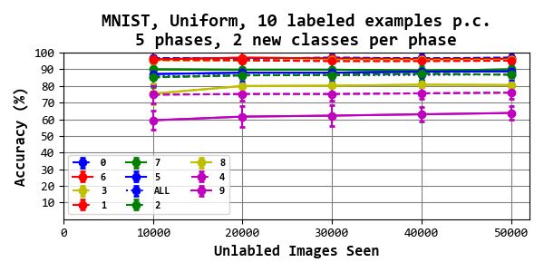
Figure 4: Classification accuracy for MNIST (left), SVHN (center), CIFAR-10 (right-center), and EMNIST (right). The task is expanding
classification for incremental UPL, i.e., recognize all classes seen so far. Note that the number of labeled examples is 10 per class (p.c.) for
MNIST and EMNIST and 100 per class for SVHN and CIFAR-10.

Classification Task: We focus on an expanding classifica-                 to the largest two receptive fields) contain the highest fraction
tion task, meaning that in each phase we need to classify all             of CIN centroids (center column of Figure 6). The ability to
classes seen so far. The results for the classification task are          recognize new classes is perhaps best visualized in the LTM
given in Figure 4. Note that we use only 10 labeled exam-                 centroid count (right column of Figure 6). During each phase
ples per class for MNIST and EMNIST, and 100 examples                     the LTM count stabilizes until a sharp spike occurs at the start
per class for SVHN and CIFAR-10. We emphasize that the                    of the next phase when new classes are introduced. This rein-
two baselines, GEM and MAS, have access to the temporal                   forces the claim that the LTM pool of centroids (i) is stable
boundaries between successive phases, while STAM does not.                when there are no new classes, and (ii) is able to recognize
   As we introduce new classes in the stream, the average                 new classes via novelty detection when they appear.
accuracy per phase decreases for all methods in each dataset.                In the CIFAR-10 experiment, the initial spike of centroids
This is expected, as the task gets more difficult after each              learned is sharp, followed by a gradual and weak increase in
phase. In MNIST, STAM performs consistently better than                   the subsequent phases. The per-class accuracy results show
GEM and MAS, and STAM is less vulnerable to catastrophic                  that STAM effectively forgets certain classes in subsequent
forgetting. For SVHN, the trend is similar after the first phase          phases (such as classes 2 and 3), suggesting that there is room
but the difference between STAM and both baselines is smaller.            for improvement in the novelty detection algorithm because
With CIFAR-10, we observe that all models including STAM                  the number of created LTM centroids was not sufficiently high.
perform rather poorly – probably due to the low resolution                   In the EMNIST experiment, as the number of classes in-
of these images. STAM is still able to maintain comparable                creases towards 47, we gradually see fewer “spikes" in the
accuracy to the baselines with a smaller memory footprint.                LTM centroids for the lower receptive fields, which is expected
Finally, in EMNIST, we see a consistently higher accuracy                 given the repetition of patterns at that small patch size. How-
with STAM compared to the two baselines. We would like to                 ever, the highly CIN layers 2 and 3 continue to recognize new
emphasize that these baselines are allowed extra information              classes and create centroids, even when the last few classes
in the form of known tasks boundaries (a label that marks                 are introduced.
when the class distribution is changing) and STAM is still
performs better both on all datasets.                                     Ablation studies: Several STAM ablations are presented in
                                                                          Figure 5. On the left, we remove the LTM capability and
6    A closer look at Incremental UPL                                     only use STM centroids for classification. During the first two
We take a closer look at STAM performance for incremental                 phases, there is little (if any) difference in classification accu-
UPL in Figure 6. As we introduce new classes to the incre-                racy. However, we see a clear dropoff during phases 3-5. This
mental UPL stream, the architecture recognizes previously                 suggests that, without the LTM mechanisms, features from
learned classes without any major degradation in classification           classes that are no longer seen in the stream are forgotten over
accuracy (left column of Figure 6). The average accuracy per              time, and STAM can only successfully classify classes that
phase is decreasing, which is due to the increasingly difficult           have been recently seen. We also investigate the importance
expanding classification task. For EMNIST, we only show                   of having static LTM centroids rather than dynamic centroids
the average accuracy because there are 47 total classes. In all           (Fig. 5-middle). Specifically, we replace the static LTM with
datasets, we observe that layer-2 and layer-3 (corresponding              a dynamic LTM in which the centroids are adjusted with the
Figure 5: Ablation study: A STAM architecture without LTM (left), a STAM architecture in which the LTM centroids are adjusted with the
same learning rate α as in STM (center), and a STAM architecture with removal of layers (right). The number of labeled examples is 100 per
class (p.c.).

same learning rate parameter α, as in STM. The accuracy suf-           pervised learning from non-stationary data with unknown task
fers drastically because the introduction of new classes “takes        boundaries. Like STAM, CURL also includes a mechanism
over" LTM centroids of previously learned classes, after the           to trigger dynamic capacity expansion as the data distribution
latter are removed from the stream. Similar to the removal of          changes. However, a major difference is that CURL is not a
LTM, we do not see the effects of “forgetting" until phases            streaming method – it processes each training example multi-
3-5. Note that the degradation due to a dynamic LTM is less            ple times. We have experimented with CURL but we found
severe than that from removing LTM completely.                         that its performance collapses in the UPL setting due to mostly
   Finally, we look at the effects of removing layers from             two reasons: the single-pass through the data requirement of
the STAM hierarchy (Fig. 5-right). We see a small drop in              UPL, and the fact that we can have more than one new classes
accuracy after removing layer 3, and a large drop in accu-             per phase. For these reasons, we choose not to compare STAM
racy after also removing layer 2. The importance of having a           with CURL because such a comparison would not be fair for
deeper hierarchy would be more pronounced in datasets with             the latter.
higher-resolution images or videos, potentially showing multi-            iLAP [Khare et al., 2021] learns classes incrementally by
ple objects in the same frame. In such cases, CIN centroids            analyzing changes in performance as new data is introduced –
can appear at any layer, starting from the lowest to the highest.      it assumes however a single new class at each transition and
                                                                       known class boundaries. [He and Zhu, 2021] investigate a
7   Related Work                                                       similar setting where pseudo-labels are assigned to new data
                                                                       based on cluster assignments but assumes knowledge of the
I: Continual learning: The main difference between most                number of classes per task and class boundaries.
continual learning approaches and STAM is that they are de-            VIII. Clustering-based representation learning: Clustering
signed for supervised learning, and it is not clear how to adapt       has been used successfully in the past for offline representation
them for online and unlabeled data streams [Aljundi et al.,            learning (e.g., [Coates et al., 2011]). Its effectiveness, however,
2018; Aljundi et al., 2019; Lopez-Paz and Ranzato, 2017].              gradually drops as the input dimensionality increases [Beyer
II. Offline unsupervised learning: These methods require               et al., 1999]. In the STAM architecture, we avoid this issue
prior information about the number of classes present in a             by clustering smaller subvectors (patches) of the input data.
given dataset and iterative training (i.e. data replay) [Bengio        If those subvectors are still of high dimensionality, another
et al., 2013].                                                         approach is to reduce the intrinsic dimensionality of the input
III. Semi-supervised learning (SSL): SSL methods require               data at each layer by reconstructing that input using represen-
labeled data during the representation learning stage [Kingma          tations (selected centroids) from the previous layer.
et al., 2014].
                                                                       IX. Other STAM components: The online clustering com-
IV. Few-shot learning (FSL) and Meta-learning: These
                                                                       ponent of STAM can be implemented with a rather simple
methods recognize object classes not seen in the training set
                                                                       recurrent neural network of excitatory and inhibitory spiking
with only a single (or handful) of labeled examples [Van-
                                                                       neurons, as shown recently [Pehlevan et al., 2017]. The nov-
schoren, 2018]. Similar to SSL, FSL methods require labeled
                                                                       elty detection component of STAM is related to the problem
data to learn representations.
                                                                       of anomaly detection in streaming data [Dasgupta et al., 2018].
V. Multi-Task Learning (MTL): Any MTL method that in-
                                                                       Finally, brain-inspired dual-memory systems have been pro-
volves separate heads for different tasks is not compatible with
                                                                       posed before for memory consolidation (e.g., [Parisi et al.,
UPL because task boundaries are not known a priori in UPL
[Ruder, 2017]. MTL methods that require pre-training on a              2018; Shin et al., 2017]).
large labeled dataset are also not applicable to UPL.                  8    Discussion
VI. Online and Progressive Learning: Many earlier meth-
ods learn in an online manner, meaning that data is processed          The STAM architecture aims to address the following desider-
in fixed batches and discarded afterwards. These methods are           ata that is often associated with Lifelong Learning:
often designed to work with supervised datastreams, stationary            I. Online learning: STAMs update the learned features
streams, or both [Venkatesan and Er, 2016].                            with every observed example. There is no separate training
VII. Unsupervised Continual Learning: Similar to the UPL               stage for specific tasks, and inference can be performed in
problem, CURL [Rao et al., 2019] focuses on continual unsu-            parallel with learning.
Figure 6: STAM Incremental UPL evaluation for MNIST (row-1), SVHN (row-2), EMNIST (row-3) and CIFAR-10 (row-4). Per-class (p.c.)
and average classification accuracy (left); fraction of CIN centroids over time (center); number of LTM centroids over time (right). The task is
expanding classification, i.e., recognize all classes seen so far.
II. Transfer learning: The features learned by the STAM Acknowledgements
architecture in earlier phases can be also encountered in the
data of future tasks (forward transfer). Additionally, new This work is supported by the Lifelong Learning Machines
centroids committed to LTM can also be closer to data of (L2M) program of DARPA/MTO: Cooperative Agreement
earlier tasks (backward transfer). HR0011-18-2-0019. The authors acknowledge the comments
of Zsolt Kira for an earlier version of this work.
III. Resistance to catastrophic forgetting: The STM-
LTM memory hierarchy of the STAM architecture mitigates References
catastrophic forgetting by committing to "permanent storage" [Aljundi et al., 2018] Rahaf Aljundi, Francesca Babiloni,
(LTM) features that have been often seen in the data during Mohamed Elhoseiny, Marcus Rohrbach, and Tinne Tuyte-
any time period of the training period. laars. Memory aware synapses: Learning what (not) to
IV. Expanding learning capacity: The unlimited capacity forget. In ECCV, 2018.
of LTM allows the system to gradually learn more features as [Aljundi et al., 2019] Rahaf Aljundi, Klaas Kelchtermans,
it encounters new classes and tasks. The relatively small size and Tinne Tuytelaars. Task-free continual learning. In
of STM, on the other hand, forces the system to forget features Proceedings of the IEEE/CVF Conference on Computer
that have not been recalled frequently enough after creation. Vision and Pattern Recognition, pages 11254–11263, 2019.
V. No direct access to previous experience: STAM only [Bengio et al., 2013] Yoshua Bengio, Aaron Courville, and
needs to store data centroids in a hierarchy of increasing re- Pascal Vincent. Representation learning: A review and
ceptive fields – there is no need to store previous exemplars or new perspectives. IEEE Trans. Pattern Anal. Mach. Intell.,
to learn a generative model that can produce such examples. 35(8):1798–1828, August 2013.[Beyer et al., 1999] Kevin S. Beyer, Jonathan Goldstein, recognition. Proceedings of the IEEE, 86(11):2278–2324, Raghu Ramakrishnan, and Uri Shaft. When is ”nearest Nov 1998. neighbor” meaningful? In Proceedings of the 7th Interna- [Lopez-Paz and Ranzato, 2017] David Lopez-Paz and tional Conference on Database Theory, ICDT ’99, pages Marc’Aurelio Ranzato. Gradient episodic memory for 217–235, London, UK, UK, 1999. Springer-Verlag. continual learning. In Proceedings of the 31st International [Coates et al., 2011] Adam Coates, Andrew Ng, and Honglak Conference on Neural Information Processing Systems, Lee. An analysis of single-layer networks in unsupervised NIPS’17, pages 6470–6479, USA, 2017. Curran Associates feature learning. In Proceedings of the fourteenth interna- Inc. tional conference on artificial intelligence and statistics, [Netzer et al., 2011] Yuval Netzer, Tao Wang, Adam Coates, pages 215–223, 2011. Alessandro Bissacco, Bo Wu, and Andrew Y. Ng. Reading [Cohen et al., 2017] Gregory Cohen, Saeed Afshar, Jonathan digits in natural images with unsupervised feature learning. Tapson, and André van Schaik. EMNIST: an extension In NIPS Workshop on Deep Learning and Unsupervised of MNIST to handwritten letters. ArXiv, abs/1702.05373, Feature Learning 2011, 2011. 2017. [Parisi et al., 2018] German I Parisi, Jun Tani, Cornelius We- [Dasgupta et al., 2018] Sanjoy Dasgupta, Timothy C Shee- ber, and Stefan Wermter. Lifelong learning of spatiotem- han, Charles F Stevens, and Saket Navlakha. A neural data poral representations with dual-memory recurrent self- structure for novelty detection. Proceedings of the National organization. Frontiers in neurorobotics, 12:78, 2018. Academy of Sciences, 115(51):13093–13098, 2018. [Pehlevan et al., 2017] Cengiz Pehlevan, Alexander Genkin, [Gidaris et al., 2018] Spyros Gidaris, Praveer Singh, and and Dmitri B Chklovskii. A clustering neural network Nikos Komodakis. Unsupervised representation learning model of insect olfaction. In 2017 51st Asilomar Confer- by predicting image rotations. In International Conference ence on Signals, Systems, and Computers, pages 593–600. on Learning Representations, 2018. IEEE, 2017. [Goldstone, 1998] Robert L Goldstone. Perceptual learning. [Rao et al., 2019] Dushyant Rao, Francesco Visin, Andrei Annual review of psychology, 49(1):585–612, 1998. Rusu, Razvan Pascanu, Yee Whye Teh, and Raia Had- [Goodfellow et al., 2013] Ian J Goodfellow, Mehdi Mirza, sell. Continual unsupervised representation learning. In Da Xiao, Aaron Courville, and Yoshua Bengio. An empiri- Advances in Neural Information Processing Systems 32, cal investigation of catastrophic forgetting in gradient-based pages 7645–7655. Curran Associates, Inc., 2019. neural networks. arXiv preprint arXiv:1312.6211, 2013. [Rebuffi et al., 2017] Sylvestre-Alvise Rebuffi, Alexander [He and Zhu, 2021] Jiangpeng He and Fengqing Zhu. Un- Kolesnikov, Georg Sperl, and Christoph H. Lampert. supervised continual learning via pseudo labels. arXiv iCaRL: Incremental classifier and representation learning. preprint arXiv:2104.07164, 2021. In 2017 IEEE Conference on Computer Vision and Pattern [Hsu et al., 2018] Yen-Chang Hsu, Yen-Cheng Liu, Anita Ra- Recognition, CVPR’17, pages 5533–5542, 2017. masamy, and Zsolt Kira. Re-evaluating continual learning [Ruder, 2017] Sebastian Ruder. An overview of multi- scenarios: A categorization and case for strong baselines. task learning in deep neural networks. arXiv preprint In NeurIPS Continual learning Workshop, 2018. arXiv:1706.05098, 2017. [Khare et al., 2021] Shivam Khare, Kun Cao, and James [Shin et al., 2017] Hanul Shin, Jung Kwon Lee, Jaehong Kim, Rehg. Unsupervised class-incremental learning through and Jiwon Kim. Continual learning with deep generative confusion. arXiv preprint arXiv:2104.04450, 2021. replay. In I. Guyon, U. V. Luxburg, S. Bengio, H. Wallach, [Kingma et al., 2014] Diederik P. Kingma, Danilo J. R. Fergus, S. Vishwanathan, and R. Garnett, editors, Ad- Rezende, Shakir Mohamed, and Max Welling. Semi- vances in Neural Information Processing Systems 30, pages supervised learning with deep generative models. In 2990–2999. Curran Associates, Inc., 2017. Proceedings of the 27th International Conference on [Vanschoren, 2018] Joaquin Vanschoren. Meta-learning: A Neural Information Processing Systems - Volume 2, survey. arXiv preprint arXiv:1810.03548, 2018. NIPS’14, pages 3581–3589, Cambridge, MA, USA, 2014. [Venkatesan and Er, 2016] Rajasekar Venkatesan and MIT Press. Meng Joo Er. A novel progressive learning technique for [Krizhevsky et al., 2014] Alex Krizhevsky, Vinod Nair, and multi-class classification. Neurocomput., 207(C):310–321, Geoffrey Hinton. The cifar-10 dataset. online: http://www. September 2016. cs. toronto. edu/kriz/cifar. html, 55, 2014. [Zeno et al., 2018] Chen Zeno, Itay Golan, Elad Hoffer, and [Kumaran et al., 2016] Dharshan Kumaran, Demis Hassabis, Daniel Soudry. Task agnostic continual learning using and James L McClelland. What learning systems do in- online variational bayes. arXiv preprint arXiv:1803.10123, telligent agents need? complementary learning systems 2018. theory updated. Trends in cognitive sciences, 20(7):512– 534, 2016. [Lecun et al., 1998] Y. Lecun, L. Bottou, Y. Bengio, and P. Haffner. Gradient-based learning applied to document
SUPPLEMENTARY MATERIAL                                               similar LTM centroids. Figure 9(f) shows that the accuracy
                                                                     remains almost the same when ∆ = 500 and |Cl | ≈ 1000.
A    STAM Notation and Hyperparameters                               Using these values we get an LTM memory size of 620000,
                                                                                    620000
All STAM notation and parameters are listed in Tables 1 - 5.         resulting in 1401540×4 ≈ 11% of GEM’s and MAS’s memory
                                                                     footprint.
B    Baseline models
                                                                     Temporary Storage and STM: We provide GEM with the
The first baseline is based on the Gradient Episodic Memories        same amount of memory as STAM’s STM. We set ∆ = 400
(GEM) model [Lopez-Paz and Ranzato, 2017] for continual              for MNIST, that is equivalent to 82 ∗ 400 + 132 ∗ 400 + 182 ∗
learning. We adapt GEM in the UPL context using the rotation-        400 = 222800 floating point values. Since the memory in
prediction self-supervised loss [Gidaris et al., 2018]. We also      GEM does not store patches but entire images, we need to
adopt the Network-In-Network architecture of [Gidaris et al.,        convert this number into images. The size of an MNIST image
2018]. The model is trained with the Adam optimizer with a           is 282 = 784, so the memory for GEM on MNIST contains
learning rate of 10−4 , batch size of 4 (the four rotations from     222800/784 ≈ 285 images. We divide this number over the
each example image), and only one epoch (to be consistent            total number of Phases – 5 in the case of MNIST – resulting in
with the streaming requirement of UPL). GEM requires knowl-          Mt = 285/5 = 57 images per task. Similarly for SVHN and
edge of task boundaries: at the end of each phase (time period       CIFAR the ∆ values are 2000 and 2500 respectively, resulting
with stationary data distribution), the model stores the Mn          in Mt ≈ 1210/5 = 242, 1515/5 = 303, and 285/23 ≈ 13
most recent examples from the training data – see [Lopez-Paz         images for SVHN, CIFAR-10, and EMNIST respectively.
and Ranzato, 2017] for more details. We set the size Mn of
the “episodic memories buffer” to the same size with STAM’s          D    Generalization Ability of LTM Centroids
STM, as described in SM-C.                                           To analyze the quality of the LTM centroids learned by STAM,
   The second baseline is based on the Memory Aware Synapse          we assess the discriminative and generalization capability of
(MAS) model [Aljundi et al., 2018] for continual learning. As        these features. For centroid c and for class k, the term gc (k)
in the case of GEM, we adapt MAS in the UPL context using            (defined in Equation 4) is the association between centroid
a rotation-prediction self-supervised loss [Gidaris et al., 2018],   c and class-k, a number between 0 and 1. The closer that
and the Network-In-Network architecture. At the end of each          metric is to 1, the better that centroid is in terms of its ability
Phase, MAS calculates the importance of each parameter on            to generalize across examples of class-k and to discriminate
the last task. These values are used in a regularization term        examples of that class from other classes.
for future tasks so that important parameters are not forgotten.        For each STAM centroid, we calculate the maximum value
Importantly, this calculation requires additional data. To make      of gc (k) across all classes. This gives us a distribution of
sure that MAS utilizes the same data with STAM and GEM,              “max-g” values for the STAM centroids. We compare that dis-
we train MAS on the first 90% of the examples during each            tribution with a null model in which we have the same number
Phase, and then calculate the importance values on the last          of LTM centroids, but those centroids are randomly chosen
10% of the data.                                                     patches from the training dataset. These results are shown Fig-
C    Memory calculations                                             ure 7. We also compare the two distributions (STAM versus
                                                                     “random examples”) using the Kolmogorov-Smirnov test. We
The memory requirement of the STAM model can be calcu-               observe that the distributions are significantly different and the
lated as:                                                            STAM centroids have higher max-g values than the random
                  Λ            Λ
                  X            X                                     examples. While there is still room for improvement (par-
            M=       ρ2l · ∆ +   ρ2l · |Cl |       (8)               ticularly with CIFAR-10), these results confirm that STAM
                      l=1           l=1
                                                                     learns better features than a model that simply remembers
where the first sum term is equivalent to the STM size and the       some examples from each class.
second sum term is the LTM size.
   We compare the LTM size of STAM with the learnable                E    Effect of unlabeled and labeled data on
parameters of the deep learning baselines. STAM’s STM, on                 STAM
the other hand, is similar GEM’s a temporary buffer, and so
we set the episodic memory storage of GEM to have the same           We next examine the effects of unlabeled and labeled data
size with STM.                                                       on the STAM architecture (Figure 8). As we vary the length
                                                                     of the unlabeled data stream (left), we see that STAMs can
Learnable Parameters and LTM: For the 3-layer SVHN                   actually perform well even with much less unlabeled data. This
architecture with |Cl | ≈ 3000 LTM centroids, the LTM                suggests that the STAM architecture may be applicable even
memory size is ≈ 1860000 pixels. This is equivalent to               where the datastream is much shorter than in the experiments
≈ 1800 gray-scale SVHN images. In contrast, the Network-             of this paper. A longer stream would be needed however if
In-Network architecture has 1401540 trainable parameters,            there are many classes and some of them are infrequent. The
which would also be stored at floating-point precision. Again,       accuracy “saturation" observed by increasing the unlabeled
with four bytes per weight, the STAM model would require             data from 20000 to 60000 can be explained based on the
  1860000
1401540×4 ≈ 33% of both GEM’s and MAS’s memory foot-                 memory mechanism, which does not update centroids after
print in terms of learnable parameters. Future work can de-          they move to LTM. As showed in the ablation studies, this
crease the STAM memory requirement further by merging                is necessary to avoid forgetting classes that no longer appear
Table 1: STAM Notation
Symbol Description
x input vector.
n dimensionality of input data
Ml number of patches at layer l (index: m = 1 . . . Ml )
xl,m m’th input patch at layer l
Cl set of centroids at layer l
cl,j centroid j at layer l
d(x, c) distance between an input vector x and a centroid c
ĉ(x) index of nearest centroid for input x
d˜l novelty detection distance threshold at layer l
U (t) the set of classes seen in the unlabeled data stream up to time t
L(t) the set of classes seen in the labeled data up to time t
k index for representing a class
gl,j (k) association between centroid j at layer l and class k.
D̄l average distance between a patch and its nearest neighbor centroid at layer l.
vl,m (k) vote of patch m at layer l for class k
vl (k) vote of layer l for class k
k(x) true class label of input x
k̂(x) inferred class label of input x
Φ(x) embedding vector of input x
Table 2: STAM Hyperparameters
Symbol Default Description
Λ 3 number of layers (index: l = 1 . . . Λ)
α 0.1 centroid learning rate
β 0.95 percentile for novelty detection distance threshold
γ 0.15 used in definition of class informative centroids
∆ see below STM capacity
θ 30 number of updates for memory consolidation
ρl see below patch dimension
Table 3: MNIST/EMNIST Architecture Table 4: SVHN Architecture Table 5: CIFAR Architecture
∆ ∆ ∆ ∆ ∆ ∆
Layer ρl (inc) (uni) Layer ρl (inc) (uni)
Layer ρl (inc) (uni)
1 8 400 2000 1 10 2000 10000 1 12 2500 12500
2 13 400 2000 2 14 2000 10000 2 18 2500 12500
3 20 400 2000 3 18 2000 10000 3 22 2500 12500
in the stream. The effect of varying the number of labeled in performance. This is likely due to the static nature of the
examples per class (right) is much more pronounced. We see LTM centroids - with low α values, the LTM centroids will
that the STAM architecture can perform well above chance primarily represent the patch they were intialized as. (b) As
even in the extreme case of only a single (or small handful of) we vary the rates of γ, there is little difference in our final
labeled examples per class. classification rates. This suggests that the maximum gl,j (k)
values are quite high, which may not be the case in other
F STAM Hyperparameter Sweeps datasets besides SVHN. (c) We observe that STAM is robust
to changes in Θ. (d,e) The STM size ∆ has a major effect
We examine the effects of STAM hyperparameters in Figure on the number of learned LTM centroids and on classification
9. (a) As we decrease the rate of α, we see a degradationFigure 7: Comparison between the distribution of max-g values with STAM and random patches extracted from the training data. Note that
the number of labeled examples is 10 per class (p.c.) for MNIST and EMNIST and 100 per class for SVHN and CIFAR-10.
Figure 8: The effect of varying the amount of unlabeled data in the entire stream (left) and labeled data per class (right). The number of
labeled examples is 100 per class (p.c.).
accuracy. (e) The accuracy in phase-5 for different numbers similarity between that class and others.
of layer-3 LTM centroids (and correspnding ∆ values). The
accuracy shows diminishing returns after we have about 1000 H Image preprocessing
LTM centroids at layer-3. (g,h) As β increases the number
Given that each STAM operates on individual image patches,
of LTM centroids increases (due to a lower rate of novelty
we perform patch normalization rather than image normaliza-
detection); if β ≥ 0.9 the classification accuracy is about the
tion. We chose a normalization operation that helps to identify
same.
similar patterns despite variations in the brightness and con-
trast: every patch is transformed to zero-mean, unit variance
G Uniform UPL before clustering. At least for the datasets we consider in this
In order to examine if the STAM architecture can learn all paper, grayscale images result in higher classification accuracy
classes simultaneously, but without knowing how many classes than color.
exist, we also evaluate the STAM architecture in a uniform We have also experimented with ZCA whitening and Sobel
UPL scenario (Figure 10). Note that LTM centroids converge filtering. ZCA whitening did not work well because it requires
to a constant value, at least at the top layer, Each class is estimating a transformation from an entire image dataset (and
recognized at a different level of accuracy, depending on the so it is not compatible with the online nature of the UPL(a) (b)
(c) (d)
(e) (f)
(g) (h)
Figure 9: Hyperparameter sweeps for α, γ, θ, β, and ∆. The number of labeled examples is 100 per class (p.c.).
problem). Sobel filtering did not work well because STAM
clustering works better with filled shapes rather than the fine
edges produced by Sobel filters.Figure 10: Uniform UPL evaluation for MNIST (row-1) and SVHN (row-2). Per-class/average classification accuracy is given at the left; the number of LTM centroids over time is given at the center; the fraction of CIN centroids over time is given at the right. Note that the number of labeled examples is 10 per class (p.c.) for MNIST and 100 per class for SVHN and CIFAR-10.
You can also read