Unsupervised Representation Learning: Autoencoders and Factorization - Ju Sun
←
→
Page content transcription
If your browser does not render page correctly, please read the page content below
Unsupervised Representation Learning:
Autoencoders and Factorization

Ju Sun
Computer Science & Engineering
University of Minnesota, Twin Cities

November 11, 2020

                                        1 / 33
Recap

  We have talked about

    – Basic DNNs (multi-layer feedforward)
    – Universal approximation theorems
    – Numerical optimization and training DNNs

                         Models and applications

    – Unsupervised representation learning: autoencoders and variants
    – DNNs for spatial data: CNNs
    – DNNs for sequential data: RNNs, LSTM
    – Generative models: variational Autoencoders and GAN
    – Interactive models: reinforcement learning

  involve modification and composition of the basic DNNs
                                                                        2 / 33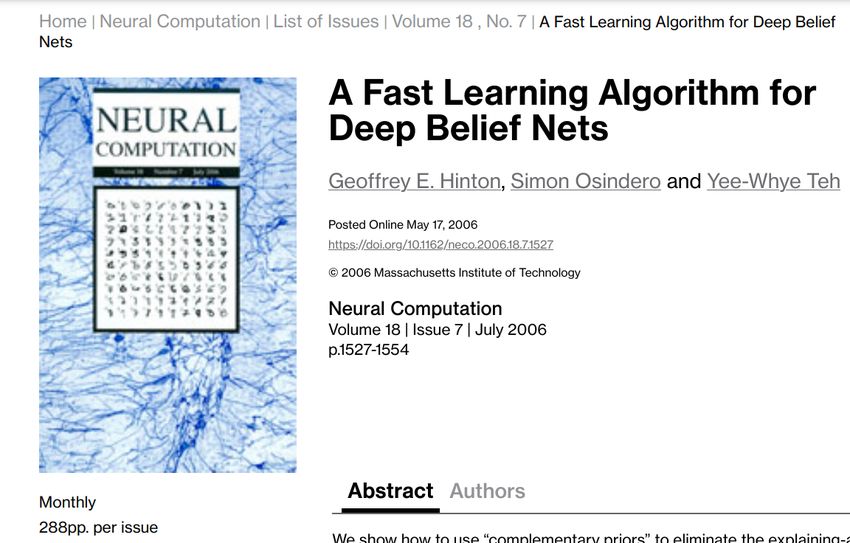
Feature engineering: old and new

                                                    Feature engineering: derive
                                                    features for efficient learning

                 Credit: [Elgendy, 2020]

   Traditional learning pipeline

      – feature extraction is “independent” of the learning models and tasks
      – features are handcrafted and/or learned

   Modern learning pipeline

      – end-to-end DNN learning
                                                                                      3 / 33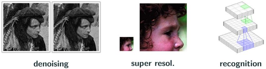
Unsupervised representation learning

   Learning feature/representation without task information (e.g., labels)
   (ICLR — International Conference on Learning Representation)

   Why not jump into the end-to-end learning?

     – Historical: Unsupervised representation learning key to the revival of deep
       learning (i.e., layerwise pretraining, [Hinton et al., 2006, Hinton, 2006])

     – Practical: Numerous advanced models built on top of the ideas in
       unsupervised representation learning (e.g., encoder-decoder networks)

                                                                                     4 / 33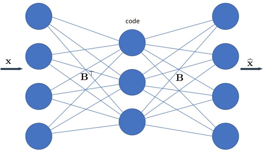
Outline

   PCA for linear data

   Extensions of PCA for nonlinear data

   Application examples

   Suggested reading

                                          5 / 33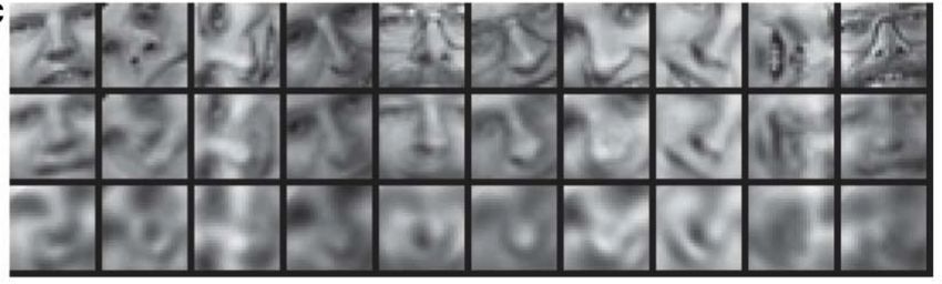
PCA: the geometric picture

   Principal component analysis (PCA)

     – Assume x1 , . . . , xn ∈ RD are zero-centered and write
       X = [x1 , . . . , xm ] ∈ RD×m
     – X = U SV | , where U spans the column space (i.e., range) of X
     – Take top singular vectors B from U , and obtain B | X

                                               – B has orthonormal columns, i.e.,
                                                 B | B = I (BB | 6= I when
                                                 D 6= d )
                                               – sample to representation:
                                                         .
                                                 x 7→ x0 = B | x (RD → Rd ,
                                                 dimension reduction)
                                               – representation to sample:
  PCA is effectively to identify the                      .
                                                 x0 7→ x
                                                       b = Bx0 (Rd → RD )
   best-fit subspace to x1 , . . . , xm
                                                 b = BB | x ≈ x
                                               – x
                                                                               6 / 33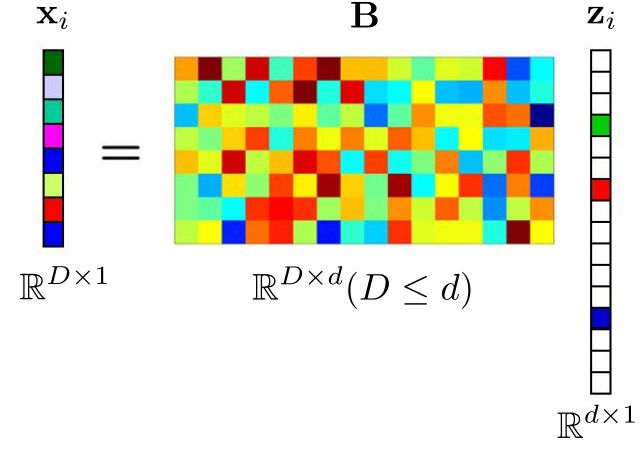
Autoencoders

  story in digital communications ...

                                        autoencoder: [Bourlard and Kamp, 1988,
                                        Hinton and Zemel, 1994]

   – Encoding:
     x 7→ x0 = B | x                    To find the basis B, solve (d ≤ D)
                                                          m
   – Decoding:                                            X
                                                   min          kxi − BB | xi k22
     x0 7→ BB | x = x
                    b                            B∈RD×d
                                                          i=1

                                                                                    7 / 33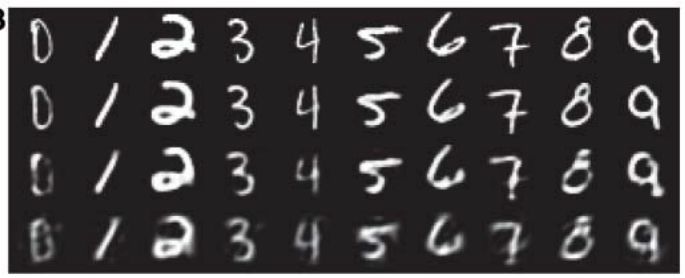
Autoencoders

 autoencoder:
                                     To find the basis B, solve
                                                           m
                                                           X
                                                    min          kxi − BB | xi k22
                                                  B∈RD×d
                                                           i=1

                                     So the autoencoder is performing PCA!

   One can even relax the weight tying:
                                          m
                                          X
                             min                kxi − BA| xi k22 ,
                       B∈RD×d ,A∈Rd×D
                                          i=1

   which finds a basis (not necessarily orthonormal) B that spans the top singular
   space also [Baldi and Hornik, 1989], [Kawaguchi, 2016],
   [Lu and Kawaguchi, 2017].

                                                                                     8 / 33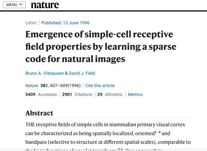
Factorization

                                      To perform PCA,
                                                               m
                                                               X
                                                         min         kxi − BB | xi k22
                                                     B∈RD×d
                                                               i=1
                                                               Xm
                                                   min               kxi − BA| xi k22 ,
                                          B∈RD×d ,A∈Rd×D
                                                               i=1

   But: the basis B and the representations/codes z i ’s are all we care about

   Factorization: (or autoencoder without encoder)
                                           m
                                           X
                                min              kxi − Bz i k22 .
                         B∈RD×d ,Z∈Rd×m
                                           i=1

   All three formulations will find three different B’s that span the same principal
   subspace [Tan and Mayrovouniotis, 1995, Li et al., 2020b, Li et al., 2020a,
   Valavi et al., 2020]. They’re all doing PCA!

                                                                                          9 / 33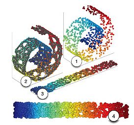
Sparse coding

   Factorization: (or autoencoder without encoder)
                                           m
                                           X
                               min               kxi − Bz i k22 .
                         B∈RD×d ,Z∈Rd×m
                                           i=1

  What happens when we allow d ≥ D? Underdetermined even if B is known.

   Sparse coding: assuming z i ’s are sparse and d ≥ D
                                   Xm                     m
                                                          X
                      min              kxi − Bz i k22 + λ   Ω (z i )
                  B∈RD×d ,Z∈Rd×m
                                     i=1                     i=1

  where Ω promotes sparsity, e.g., Ω = k·k1 .

                                                                          10 / 33
More on sparse coding
also known as (sparse) dictionary learning [Olshausen and Field, 1996,
Mairal, 2014, Sun et al., 2017, Bai et al., 2018, Qu et al., 2019]
11 / 33Outline
PCA for linear data
Extensions of PCA for nonlinear data
Application examples
Suggested reading
12 / 33Quick summary of the linear models
– B from U of X = U SV |
– autoencoder:
Pm | 2
minB∈RD×d i=1 kxi − BB xi k2
– autoencoder:
Pm | 2
minB∈RD×d ,A∈Rd×D i=1 kxi − BA xi k2
PCA is effectively to identify
the best-fit subspace to – factorization:
Pm 2
x1 , . . . , xm minB∈RD×d ,Z∈Rd×m i=1 kxi − Bz i k2
– when d ≥ D, sparse coding/dictionary
learning
m
X m
X
min kxi − Bz i k22 + λ Ω (z i )
B∈RD×d ,Z∈Rd×m
i=1 i=1
e.g., Ω = k·k1
13 / 33What about nonlinear data?
– Manifold, but not mathematically (i.e., differential geomety sense) rigorous
– (No. 1?) Working hypothesis for high-dimensional data: practical
data lie (approximately) on union of low-dimensional “manifolds”. Why?
* data generating processes often controlled by very few parameters
14 / 33Manifold learning
Classic methods (mostly for visualization): .e.g.,
– ISOMAP [Tenenbaum, 2000]
– Locally-Linear Embedding [Roweis, 2000]
– Laplacian eigenmap [Belkin and Niyogi, 2001]
– t-distributed stochastic neighbor embedding
(t-SNE) [van der Maaten and Hinton, 2008]
Nonlinear dimension reduction and representation learning
15 / 33From autoencoders to deep autoencoders
m
X
min kxi − BB | xi k22
B∈RD×d
i=1
Xm
min kxi − BA| xi k22
B∈RD×d ,A∈Rd×D
i=1
nonlinear generalization of the linear mappings:
deep autoencoders
m
X
min kxi − gV ◦ fW (xi )k22
V ,W
i=1
simply A| → fW and B → gV
A side question: why not calculate “nonlinear basis”?
16 / 33Deep autoencoders
m
X
min kxi − gV ◦ fW (xi )k22
V ,W
i=1
the landmark paper [Hinton, 2006] ... that introduced pretraining
17 / 33From factorization to deep factorization
factorization
m
X
min kxi − Bz i k22
B∈RD×d ,Z∈Rd×m
i=1
nonlinear generalization of the linear mappings:
deep factorization
m
X
min kxi − gV (z i )k22
V ,Z∈Rd×m
i=1
simply B → gV
[Tan and Mayrovouniotis, 1995, Fan and Cheng, 2018, Bojanowski et al., 2017,
Park et al., 2019, Li et al., 2020b], also known as deep decoder.
18 / 33From sparse coding to deep sparse coding
– when d ≥ D, sparse coding/dictionary
learning
m
X m
X
min kxi − Bz i k22 + λ Ω (z i )
B∈RD×d ,Z∈Rd×m
i=1 i=1
e.g., Ω = k·k1
nonlinear generalization of the linear mappings: (d ≥ D)
deep sparse coding/dictionary learning
m
X m
X
min kxi − gV (z i )k22 + λ Ω (z i )
V ,Z∈Rd×m
i=1 i=1
Xm m
X
min kxi − gV ◦ fW (xi )k22 + Ω (fW (xi ))
V ,W
i=1 i=1
the 2nd also called sparse autoencoder [Ranzato et al., 2006].
19 / 33Quick summary of linear vs nonlinear models
linear models nonlinear models
Pm
minB ` (xi , BB | xi ) Pm
autoencoder Pi=1
m | minV ,W i=1 ` (xi , gV ◦ fW (xi ))
minB,A i=1 ` (xi , BA xi )
P m Pm
factorization minB,Z i=1 ` (xi , Bz i ) minV ,Z i=1 ` (xi , gV (z i ))
Pm
minV ,Z i=1 ` (xi , gV (z i ))
Pm
+λ m
P
minB,Z i=1 ` (xi , Bz i ) i=1 Ω (z i )
sparse coding Pm Pm
+λ i=1 Ω (z i ) minV ,W i=1 ` (xi , gV ◦ fW (xi ))
+λ m
P
i=1 Ω (fW (xi ))
` can be general loss functions other than k·k2
Ω promotes sparsity, e.g., Ω = k·k1
20 / 33Outline
PCA for linear data
Extensions of PCA for nonlinear data
Application examples
Suggested reading
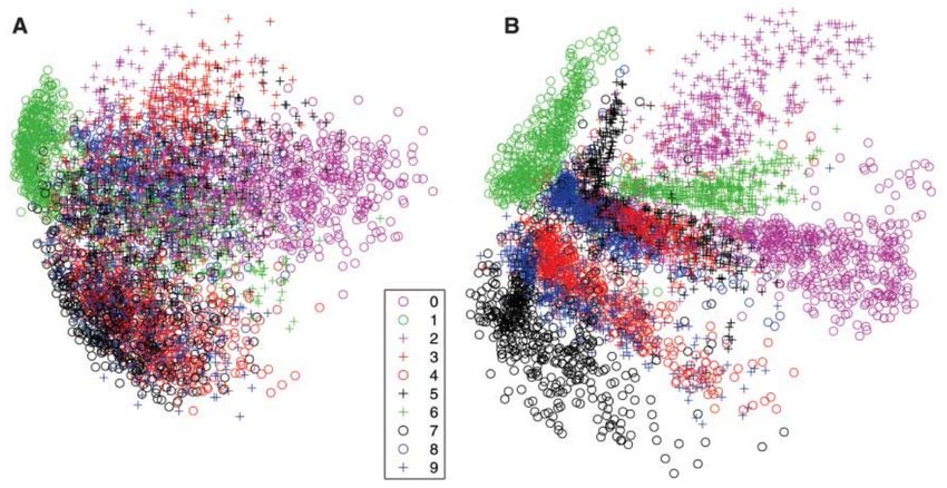
21 / 33Nonlinear dimension reduction
autoencoder vs. PCA vs. logistic PCA
[Hinton, 2006]
22 / 33Representation learning
Traditional learning pipeline
– feature extraction is “independent” of the learning models and tasks
– features are handcrafted and/or learned
Use the low-dimensional codes as features/representations
– task agnostic
– less overfitting
– semi-supervised (rich unlabeled data + little labeled data) learning
23 / 33Outlier detection
(Credit: towardsdatascience.com)
– idea: outliers don’t obey the manifold assumption — the reconstruction
error ` (xi , gV ◦ fW (xi )) is large after autoencoder training
– for effective detection, better use ` that penalizes large errors less harshly
than k·k22 , e.g., ` (xi , gV ◦ fW (xi )) = kxi − gV ◦ fW (xi )k2
[Lai et al., 2019]
24 / 33Deep generative prior
– inverse problems: given f and y = f (x),
estimate x
– often ill-posed, i.e., y doesn’t contain
enough info for recovery
– regularized formulation:
min ` (y, f (x)) + λΩ (x)
x
where Ω contains extra info about x
Suppose x1 , . . . , xm come from the same manifold as x
– train a deep factorization model on x1 , . . . , xm :
Pm
minV ,Z i=1 ` (xi , gV (z i ))
– x ≈ gV (z) for a certain z so: minz ` (y, f ◦ gV (z)) . Some recent work
even uses random V , i.e., without training
[Ulyanov et al., 2018, Bora and Dimakis, 2017]
25 / 33To be covered later
– convolutional encoder-decoder networks (i.e., segmentation, image
processing, inverse problems)
– autoencoder sequence-to-sequence models (e.g., machine translation)
– variational autoencoders (generative models)
26 / 33Outline
PCA for linear data
Extensions of PCA for nonlinear data
Application examples
Suggested reading
27 / 33Suggested reading
– Representation Learning: A Review and New Perspectives (Bengio, Y.,
Courville, A., and Vincent, P.) [Bengio et al., 2013]
– Chaps 13–15 of Deep Learning [Goodfellow et al., 2017].
– Rethink autoencoders: Robust manifold learning [Li et al., 2020b]
28 / 33References i
[Bai et al., 2018] Bai, Y., Jiang, Q., and Sun, J. (2018). Subgradient descent learns
orthogonal dictionaries. arXiv:1810.10702.
[Baldi and Hornik, 1989] Baldi, P. and Hornik, K. (1989). Neural networks and
principal component analysis: Learning from examples without local minima.
Neural Networks, 2(1):53–58.
[Belkin and Niyogi, 2001] Belkin, M. and Niyogi, P. (2001). Laplacian eigenmaps and
spectral techniques for embedding and clustering. In Dietterich, T. G., Becker, S.,
and Ghahramani, Z., editors, Advances in Neural Information Processing Systems
14 [Neural Information Processing Systems: Natural and Synthetic, NIPS 2001,
December 3-8, 2001, Vancouver, British Columbia, Canada], pages 585–591. MIT
Press.
[Bengio et al., 2013] Bengio, Y., Courville, A., and Vincent, P. (2013).
Representation learning: A review and new perspectives. IEEE Transactions on
Pattern Analysis and Machine Intelligence, 35(8):1798–1828.
[Bojanowski et al., 2017] Bojanowski, P., Joulin, A., Lopez-Paz, D., and Szlam, A.
(2017). Optimizing the latent space of generative networks. arXiv:1707.05776.
29 / 33References ii
[Bora and Dimakis, 2017] Bora, Ashish, A. J. E. P. and Dimakis, A. G. (2017).
Compressed sensing using generative models. In Proceedings of the 34th
International Conference on Machine Learning, volume 70.
[Bourlard and Kamp, 1988] Bourlard, H. and Kamp, Y. (1988). Auto-association by
multilayer perceptrons and singular value decomposition. Biological Cybernetics,
59(4-5):291–294.
[Elgendy, 2020] Elgendy, M. (2020). Deep Learning for Vision Systems. MANNING
PUBN.
[Fan and Cheng, 2018] Fan, J. and Cheng, J. (2018). Matrix completion by deep
matrix factorization. Neural Networks, 98:34–41.
[Goodfellow et al., 2017] Goodfellow, I., Bengio, Y., and Courville, A. (2017). Deep
Learning. The MIT Press.
[Hinton, 2006] Hinton, G. E. (2006). Reducing the dimensionality of data with
neural networks. Science, 313(5786):504–507.
[Hinton et al., 2006] Hinton, G. E., Osindero, S., and Teh, Y.-W. (2006). A fast
learning algorithm for deep belief nets. Neural Computation, 18(7):1527–1554.
30 / 33References iii
[Hinton and Zemel, 1994] Hinton, G. E. and Zemel, R. S. (1994). Autoencoders,
minimum description length and helmholtz free energy. In Advances in neural
information processing systems, pages 3–10.
[Kawaguchi, 2016] Kawaguchi, K. (2016). Deep learning without poor local minima.
arXiv:1605.07110.
[Lai et al., 2019] Lai, C.-H., Zou, D., and Lerman, G. (2019). Robust subspace
recovery layer for unsupervised anomaly detection. arXiv:1904.00152.
[Li et al., 2020a] Li, S., Li, Q., Zhu, Z., Tang, G., and Wakin, M. B. (2020a). The
global geometry of centralized and distributed low-rank matrix recovery without
regularization. arXiv:2003.10981.
[Li et al., 2020b] Li, T., Mehta, R., Qian, Z., and Sun, J. (2020b). Rethink
autoencoders: Robust manifold learning. ICML workshop on Uncertainty and
Robustness in Deep Learning.
[Lu and Kawaguchi, 2017] Lu, H. and Kawaguchi, K. (2017). Depth creates no bad
local minima. arXvi:1702.08580.
[Mairal, 2014] Mairal, J. (2014). Sparse modeling for image and vision processing.
Foundations and Trends® in Computer Graphics and Vision, 8(2-3):85–283.
31 / 33References iv
[Olshausen and Field, 1996] Olshausen, B. A. and Field, D. J. (1996). Emergence of
simple-cell receptive field properties by learning a sparse code for natural images.
Nature, 381(6583):607–609.
[Park et al., 2019] Park, J. J., Florence, P., Straub, J., Newcombe, R., and Lovegrove,
S. (2019). Deepsdf: Learning continuous signed distance functions for shape
representation. pages 165–174. IEEE.
[Qu et al., 2019] Qu, Q., Zhai, Y., Li, X., Zhang, Y., and Zhu, Z. (2019). Analysis of
the optimization landscapes for overcomplete representation learning.
arXiv:1912.02427.
[Ranzato et al., 2006] Ranzato, M., Poultney, C. S., Chopra, S., and LeCun, Y.
(2006). Efficient learning of sparse representations with an energy-based model.
In Advances in Neural Information Processing Systems.
[Roweis, 2000] Roweis, S. T. (2000). Nonlinear dimensionality reduction by locally
linear embedding. Science, 290(5500):2323–2326.
[Sun et al., 2017] Sun, J., Qu, Q., and Wright, J. (2017). Complete dictionary
recovery over the sphere i: Overview and the geometric picture. IEEE
Transactions on Information Theory, 63(2):853–884.
32 / 33References v
[Tan and Mayrovouniotis, 1995] Tan, S. and Mayrovouniotis, M. L. (1995). Reducing
data dimensionality through optimizing neural network inputs. AIChE Journal,
41(6):1471–1480.
[Tenenbaum, 2000] Tenenbaum, J. B. (2000). A global geometric framework for
nonlinear dimensionality reduction. Science, 290(5500):2319–2323.
[Ulyanov et al., 2018] Ulyanov, D., Vedaldi, A., and Lempitsky, V. (2018). Deep
image prior. In Proceedings of the IEEE Conference on Computer Vision and
Pattern Recognition, pages 9446–9454.
[Valavi et al., 2020] Valavi, H., Liu, S., and Ramadge, P. J. (2020). The landscape of
matrix factorization revisited. arXiv:2002.12795.
[van der Maaten and Hinton, 2008] van der Maaten, L. and Hinton, G. (2008).
Visualizing data using t-sne. Journal of Machine Learning Research, 9:2579–2605.
33 / 33You can also read


