USING A DIGITAL CAMERA TO STUDY MOTION - ANDREW J. MCNEIL AND STEVEN DANIEL
←
→
Page content transcription
If your browser does not render page correctly, please read the page content below
McNeil and Daniel                      Using a digital camera to study motion

            Using a digital camera to
                        study motion
                                   Andrew J. McNeil and Steven Daniel

  A digital camera is an excellent device for recording a range of motions
     and interactions of objects – SHM, free-fall, and elastic and inelastic
                        collisions – so they can subsequently be analysed

Some of our earliest conscious interactions with the            article show selected frames from the video record
physical world involve forces on objects, and their             taken in lessons, and hence show other features like
consequent motion. As children, we soon become                  lab taps, and what was on display boards at the time.
skilled at applying just the right force for just the right     The video frames have been augmented in Microsoft
duration to produce the desired motion. Galileo’s               Word, with the addition of features such as scales
study of the motion of balls rolling down slopes was            and dimensions.
one of the earliest mathematical analyses of terrestrial            The work described here was triggered by the
motion (Gribbin, 2002: 101). Yet motion remains                 demise of our department’s last BBC ‘B’ computer,
difficult to observe and quantify. Ticker-timers,               and also by one of us (AJM) discovering the delights
light gates and motion sensors of various types will            and power of digital photography. When we found
continue to be useful. This article describes how we            out how easy it was to analyse the simple harmonic
have used a digital camera to record and analyse                motion (shm) of a mass oscillating on a spring, we
motion in various situations, as part of an A-level             went on to look at projectiles and collisions.
physics course. The camera used was an Olympus
C360Z. This records video in Quicktime format, at
15 frames per second (fps) with a frame size of 320 x           Simple harmonic motion (shm)
240 pixels, giving a reasonable degree of resolution,           Students are very familiar with everyday examples
sufficient to measure the position of a pointer to the          of shm, from the simple pendulum to the bungee
nearest centimetre. The video can be viewed frame               jumper. A computer and rotational position sensor
by frame, using Olympus or Apple software. The file             can be used to record the motion of a mass oscillating
sizes are quite small, being about 0.3 MB for every 1           on a spring. We started by seeing if we could do this
second (15 frames) of video. The photographs in this            with the digital camera.
                                                                    Figure 1 shows the simple experimental arrange-
                                                                ment. The camera was placed on a level surface at
    ABSTRACT                                                    the same height as the scale, and about 1 metre away,
    A digital camera can easily be used to make                 close enough to measure position to ± 0.5 cm, but not
    a video record of a range of motions and                    so close as to introduce serious parallax errors. There
    interactions of objects – shm, free-fall and                was no need to synchronise the camera with the
    collisions, both elastic and inelastic. The video           action. We set the mass oscillating, let it settle for a
    record allows measurements of displacement                  few cycles, and then started the camera and recorded
    and time, and hence calculation of velocities,              the motion for a further 2–3 cycles. The time period
    and practice with the standard formulas for                 of about 1 second was long enough to resolve one
    motions and collisions. The camera extends the              cycle, frame by frame. The centre of the oscillation
    range of motions that can be studied, to include
                                                                was measured, from which the displacement every
    free-fall with forward motion and collisions
    between two moving objects. The exercise                    1/15th of a second could easily be recorded. An
    gives students valuable experience in handling              improvement on this arrangement would be to have
    raw data, and brings a concrete experience                  a scale with a central zero, and to position the resting
    to a part of physics that is sometimes treated              mass with the pointer at zero.
    theoretically.

                                                              School Science Review, September 2006, 88(322)      123
Using a digital camera to study motion McNeil and Daniel
Figure 1 A frame from the video
of an oscillating 600 g mass. The
reading of the pointer is 8.5 cm on
the scale.
We have used these data with students to work Projectiles
with the shm equations. Students calculated the
time period from the video, and checked it against We then went on to use the camera to record the motion
direct measurement with a stopclock. They used of a free-falling projectile. We used the arrangement
the relationship between time period and spring shown in Figure 2 to produce a predetermined initial
constant, velocity, followed by free-fall under gravity. The
ball’s trajectory was very close to the wall, ending
m on the side bench. This reduced parallax errors in
T= 2≠
= 2π (1)
k measuring positions, and also ensured that students
were kept well out of the way. Demonstrations using
where T is the time period (s), m is the oscillating mass faster and/or heavier projectiles and longer ranges
(kg), and k is the spring constant (N m–1), to check would need an appropriate risk assessment. The ball
the value of k agreed with the manufacturer’s data. was held in contact with the ramp, and then released,
The maximum velocity, vmax (m s–1), at the centre of to minimise the chance of sliding as it rolled down
the oscillation can be measured and checked against the ramp.
the value calculated, using the formula, The video record can be used to plot the ball’s
vmax = 2πfA (2) motion on the scale, using blobs of sticky tack.
Students can see the vertical component of motion
where f is the frequency (Hz), calculated as f = 1/T, increase, while the horizontal component stays
and A is the amplitude (m). constant. The ball hit the bench between frames 7 and
The expression for the displacement, x/m, of the 8, making the time of flight very close to 0.50 s.
oscillating mass at any time t/s, We can use the kinematics equation,
x = A cos(2πft) (3) s = ut + 12 gt 2
(4)
often gives students difficulties. Points can be on the vertical component of motion, where s is the
selected from the video record to check the calculated displacement (m), u is the initial vertical velocity (m
displacements, both negative and positive. We have s–1) – equal to zero in this case – and t is the time of
found calculations to agree with measurements from flight (s) under gravitational acceleration, g (taken
the video record to within about 10 per cent. as 9.8 m s–2). This tells us that the ball has fallen
Students enjoy getting involved in reading the through a vertical height of 1.2 m, in very good
video record, and checking the formulas – which agreement with the scale on the wall.
many feel initially are highly abstract – against a The ball travelled close to 55 cm horizontally
very tangible physical experience. during its free fall, so the velocity formula,
vh = s/t (5)
gives the horizontal velocity, vh, as 1.1 m s–1.
124 School Science Review, September 2006, 88(322)McNeil and Daniel Using a digital camera to study motion
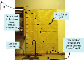
Figure 2 A small steel ball is
rolled down the ramp R, placed
on top of the wall cupboard.
The blurred object at position
‘0’ is the ball leaving the end
of the ramp with a horizontal
velocity. The ball’s subsequent
free-fall to the bench is shown
by the black circles, some of
which are marked with their
frame numbers. Axes have
been added to the digital
video frame. The camera was
positioned about 2 m away,
level with the centre of the
scale on the wall. There is some
parallax error at the top and
bottom of the scale.
How does this compare with the velocity of the where I (kg m2) is the moment of inertia, and ω
ball when rolled down the ramp on to a horizontal (rad s–1) is the angular velocity. Since the moment
bench? The video record, shown in Figure 3, gives of inertia of a solid sphere is 0.4mr2 (Nelkon and
the horizontal velocity, vh, as about 1.2 m s–1, in good Parker, 1995: 120; Tipler and Mosca, 2004), and
agreement with the motion under free fall. ω = vh/r, expression (7) helpfully becomes:
Does this velocity tally with the measured height
Ek(r) = 0.2mvh2 (8)
of the ramp? The first step is to use the simple
(GCSE) relationship between initial potential and Expression (6) now becomes (Nelkon and Parker,
final kinetic energy of the ball (where the mass of 1995: 120):
the ball is m kg):
mgh = 0.5mvh2 + 0.2mvh2 (9)
mgh = 2 mvh
1 2
(6)
The ball’s rotational kinetic energy Ek(r) is nearly
The ramp’s measured height of 0.11 m should give equal to half of its linear kinetic energy. Taking
the ball a horizontal velocity of about 1.5 m s–1. This height h = 0.11 m gives a predicted value of velocity
clearly exceeds the measured velocity, so where has vh of 1.2 m s–1, close to the two measured values.
some of the potential energy gone?
You can use the disparity to help students see
that the rolling ball has both linear and rotational Collisions
kinetic energy. The rotational kinetic energy Ek(r) is We finally turned to studying momentum changes in
given by collisions. Here we found the camera brought a real
Ek(r) = 0.5Iω2 (7) bonus. In the past we have taught momentum using
Figure 3 The same ball is rolled down the same ramp on to the horizontal bench. In 8 video frames (8/15ths
of a second) the ball rolls about 62 cm, from 3 cm to 65 cm on the scale behind.
School Science Review, September 2006, 88(322) 125Using a digital camera to study motion McNeil and Daniel
Figure 4 Two gliders
are pushed to approach
each other on the air
track. Each carries a
short vertical pencil stuck
on with sticky tack, to
record its position. Just
behind the air track is a
horizontal scale, with 5
cm markings, enabling
positions to be read to
the nearest cm.
light gates or motion sensors, using the standard data from the video frame by frame, and recording
gliders on an air track. The limitations on equipment their calculations on the board, checking each others’
available to us meant that we could measure the working as they go. Students appreciate seeing a
velocity of only one glider, restricting us to inelastic macroscopic version of an intermolecular collision
collisions with one glider initially at rest. With that can be related to the kinetic theory of ideal
the camera we could record elastic and inelastic gases. They also see the need for a sign convention,
collisions between two moving gliders. for the pattern to emerge.
We were able to study elastic collisions, where Table 1 gives a typical set of results for an elastic
the mutual repulsion of the magnets prevented the collision on a carefully levelled track. They show
gliders making contact, and also wholly inelastic the conservation of momentum and kinetic energy
collisions, where the gliders were locked together to within about 10 per cent. We offer only one set of
by the magnets’ attraction. Glider velocities were results, to illustrate the typical values and precision
calculated simply by measuring their displacement that can be achieved.
in a known time, usually a few video frames. It was Inelastic collisions, as shown in Figure 6, can
found to be important to measure velocities close to be treated the same way. Handling the gliders, and
the moment of impact, to get accurate results. We seeing the magnets attracting and colliding helps
found that with 5 cm divisions we could reasonably students to appreciate the transfer of kinetic energy
estimate positions to the nearest centimetre. Figure 4 to internal energy.
shows the experimental arrangement. It is quite straightforward to simulate explosions,
Figure 5 shows the aftermath of an elastic collis- by tying two repelling gliders together with thread,
ion. Measuring velocities of both gliders before and burning through the thread, and recording the
after this type of collision – four values – shows that gliders’ motions. You can start with the tied gliders
the system of gliders suffers no loss of momentum or at rest, simulating firing a gun, or in motion, perhaps
kinetic energy. It is important to use small approach simulating the separation of a satellite and its booster
velocities, to ensure the magnets do not make rocket.
contact. As before, the students enjoy reading the
Figure 5 After an
elastic collision, the
two gliders move
apart. The velocity of
each can be measured
against the scale
behind.
126 School Science Review, September 2006, 88(322)McNeil and Daniel Using a digital camera to study motion
Table 1
Glider A mass = 0.39 kg. Glider B mass = 0.57 kg Totals
Before collision Before collision
moved from 39 to 48 cm in 5 moved from 115 to 109 cm in 7
frames. Velocity = 0.27 m s–1. frames. Velocity = – 0.13 m s–1.
Momentum Momentum Total momentum
= mv = +0.11 kg m s–1 = mv = – 0.074 kg m s–1 = + 0.036 kg m s–1
Kinetic energy Kinetic energy Total Ek
= + 0.014 J = + 0.005 J = + 0.019 J
After collision After collision
moved from 73 to 63 cm in 7 moved from 110 to 117 cm in 5
frames. Velocity = – 0.21 m s–1. frames. Velocity = 0.21 m s–1.
Momentum Momentum Total momentum
= mv = – 0.082 kg m s–1 = mv = +0.12 kg m s–1 = + 0.038 kg m s–1
Kinetic energy Kinetic energy Total Ek
= + 0.009 J = + 0.013 J = + 0.022 J
Figure 6 After an inelastic
collision, the two gliders
move as one object, held
together by the magnets.
Conclusion
Many modern digital cameras can record in video situations. They get ‘hands on’ experience of making
mode. This allows physics students to record measurements, and seeing the patterns emerge. This
and analyse the motion of objects in a variety of simple video recording can greatly help students’
understanding of the physics of forces and motion.
References
Gribbin, J. (2002) Science: a history, 1534–2001. London: Tipler, P. A. and Mosca, G. (2004) Physics for scientists and
BCA (Penguin). engineers. 5th edn. New York: W. H. Freeman.
Nelkon, M. and Parker, P. (1995) Advanced level physics. 7th
edn. London: Heinemann.
Andrew James McNeil is now retired from teaching, but still very interested in science teaching, and
thinking and learning skills in all aspects of education. He last taught at Wilsthorpe Business and Enterprise
College, Long Eaton, Nottingham where co-author Steven Daniel currently teaches.
Email: mcneilaandh@hotmail.com
School Science Review, September 2006, 88(322) 127You can also read