Validating Morphometrics with DNA Barcoding to Reliably Separate Three Cryptic Species of Bombus Cresson (Hymenoptera: Apidae) - MDPI
←
→
Page content transcription
If your browser does not render page correctly, please read the page content below
insects
Article
Validating Morphometrics with DNA Barcoding to
Reliably Separate Three Cryptic Species of Bombus
Cresson (Hymenoptera: Apidae)
Joan Milam 1, *, Dennis E. Johnson 2,† , Jeremy C. Andersen 1 , Aliza B. Fassler 1 ,
Desiree L. Narango 1 and Joseph S. Elkinton 1
 1    Department of Environmental Conservation, University of Massachusetts Amherst, 160 Holdsworth Way,
      Amherst, MA 01003, USA; jcandersen@umass.edu (J.C.A.); alizamfassler@gmail.com (A.B.F.);
      dnarango@gmail.com (D.L.N.); elkinton@ent.umass.edu (J.S.E.)
 2    Private Practice, Eau Claire, WI 54701, USA; dermjohn@aol.com
 *    Correspondence: jmilam@umass.edu; Tel.: +1-9787-302-6499
 †    Currently retired.

 Received: 14 September 2020; Accepted: 27 September 2020; Published: 30 September 2020

 Simple Summary: Evidence of bumble bee population declines has led to an increase in conservation
 efforts to protect these important pollinators. However, effective conservation requires accurate
 species identification. We provide quantitative methods to accurately identify three cryptic species
 of bumble bees using morphometric measurements of the cheek length and width, and antennal
 segments. We validated the accuracy of our methods with DNA analysis. We predicted that these
 methods would reliably identify both the queens and worker bees of Bombus vagans and B. sandersoni.
 We expanded these methods to include an uncommon form of Bombus perplexus with all light hair on
 its thorax, rather than the more common light on top and dark below, that can mistakenly be identified
 as B. vagans or B. sandersoni. Although the species we consider here, Bombus vagans, B. sandersoni and
 B. perplexus, are not currently listed as species of concern in North America, there is uncertainty of
 their population status, some of which is due to difficulty in species identification, which we have
 resolved. Recent history informs us that some bumble bee species experience rapid declines within a
 few decades. Our methods to correctly identify these cryptic species is key to monitoring their status
 and population trends.

 Abstract: Despite their large size and striking markings, the identification of bumble bees (Bombus spp.)
 is surprisingly difficult. This is particularly true for three North American sympatric species in the
 subgenus Pyrobombus that are often misidentified: B. sandersoni Franklin, B. vagans Smith B. perplexus
 Cresson. Traditionally, the identification of these cryptic species was based on observations of
 differences in hair coloration and pattern and qualitative comparisons of morphological characters
 including malar length. Unfortunately, these characteristics do not reliably separate these species.
 We present quantitative morphometric methods to separate these species based on the malar length
 to width ratio (MRL) and the ratios of the malar length to flagellar segments 1 (MR1) and 3 (MR3)
 for queens and workers, and validated our determinations based on DNA barcoding. All three
 measurements discriminated queens of B. sandersoni and B. vagans with 100% accuracy. For workers,
 we achieved 99% accuracy by combining both MR1 and MR3 measurements, and 100% accuracy
 differentiating workers using MRL. Moreover, measurements were highly repeatable within and
 among both experienced and inexperienced observers. Our results, validated by genetic evidence,
 demonstrate that malar measurements provide accurate identifications of B. vagans and B. sandersoni.
 There was considerable overlap in the measurements between B. perplexus and B. sandersoni. However,
 these species can usually be reliably separated by combining malar ratio measurements with other
 morphological features like hair color. The ability to identify bumble bees is key to monitoring the
 status and trends of their populations, and the methods we present here advance these efforts.

Insects 2020, 11, 669; doi:10.3390/insects11100669                             www.mdpi.com/journal/insects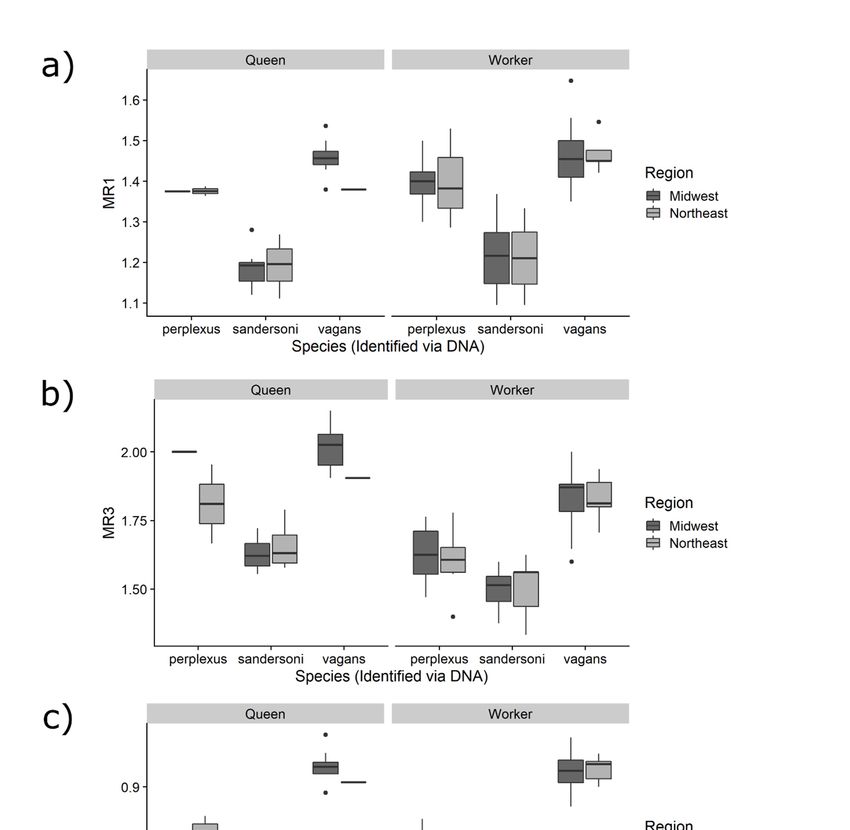
Insects 2020, 11, 669                                                                                 2 of 20

 Keywords: Apoidea; Bombini; malar ratio; Bombus vagans; Bombus sandersoni; Bombus perplexus

1. Introduction
      Recent reports of major declines in global insect populations are cause for concern [1–4].
While declines are occurring in nearly all groups of insects, severe declines have been noted in
wild bee populations [5], particularly bumble bees Bombus Cresson (Hymenoptera: Apidae) since the
mid-twentieth century [6–14]. These declines have been attributed to a wide range of factors including
habitat loss and fragmentation, climate change, intensified use of pesticides in agriculture, loss of floral
resources, disease, and invasive species [6–10,15,16]. Evident declines in the range and abundance
in bumble bee populations have encouraged increased research efforts to document distribution,
population status and trends, extinction risks, and best management practices [5,12,14,17–19].
      Unfortunately, despite being large-bodied with conspicuous hair coloration and patterns,
many bumble bee species are deceptively challenging to identify [20–23], particularly because there are
few helpful characters for separating species [24]. In North America, several identification guides exist
for bumble bees [23,25–27], however, there are still challenges to the identification of some similarly
colored cryptic species. Hair coloration is an important field characteristic for identification, yet it has
been widely acknowledged that accurate identifications based on hair coloration are complicated by
chromatic variability within species and convergent evolution between species [23,28–30]. For example,
Franklin [25] confessed that he had “much difficulty in describing the colors exhibited by the pile
of the various species.” Therefore, errors in identification may result without careful examination of
morphological characters [28,31,32].
      Three commonly misidentified sympatric species of bumble bee with similar hair coloration and
patterns in the subgenus Pyrobombus Dalla Torre, are B. vagans (Half-Black Bumble Bee), B. sandersoni
(Sanderson Bumble Bee) and B. perplexus (Confusing Bumble Bee). While hair color has frequently
been used in bumble bee identification, there exists considerable variation in hair color patterns both
within and among castes of B. sandersonii, B. vagans and B. perplexus [23,25,27], making reliance on this
character alone insufficient. Although B. perplexus typically has extensive black hair on the lower half
of the pleura [25,27], it has a less common light colored form that has the sides of the thorax entirely
yellow to the base of the legs that is often confused with the prior two species [23]. Franklin [25] stated
that light form females of B. perplexus were regularly confused as B. vagans.
      In addition to their morphologic similarities, these species share a confusing history that is
complicated by the fact that important early taxonomic work on this group was conducted solely
on spring-caught queens and males [25,28]. Franklin initially described B. sandersoni as a subspecies
of B. vagans noting slight differences in their malar space. Frison [33] did not agree with Franklin’s
determinations that B. sandersoni was a subspecies of B. vagans and instead suggested that B. sandersoni
was actually a color variety of B. frigidus Smith based on his observations of the male genitalia [28].
Later, Mitchell [27] and Soroye and Bucks [34] classified B. sandersoni as a separate species from
B. vagans, also based on differences in the malar length in spring-caught queens [28].
      To reliably separate these species, previous authors sought to find morphologic characters
that were consistent across a range of body sizes and castes to reliably differentiate species in the
subgenus Pyrobombus. For example, Plowright and Pallett [28] proposed that spring-caught queen
B. sandersoni, B. vagans, and B. frigidus specimens from a wide geographic range across Canada could
be identified using several metrics including wing venation, and measurements of malar and antennal
lengths. Following the methods in Richards [31], they verified that the length of malar spaces in
spring-caught queen B. vagans did not overlap with either queen B. sandersoni or B. frigidus, but that
the malar space did not significantly separate the queens of B. frigidus from B. sandersoni, concluding
that the relationship between B. sandersoni and B. frigidus remained unclear and required further
investigation [28]. They acknowledged that the longer malar length of B. vagans was the primary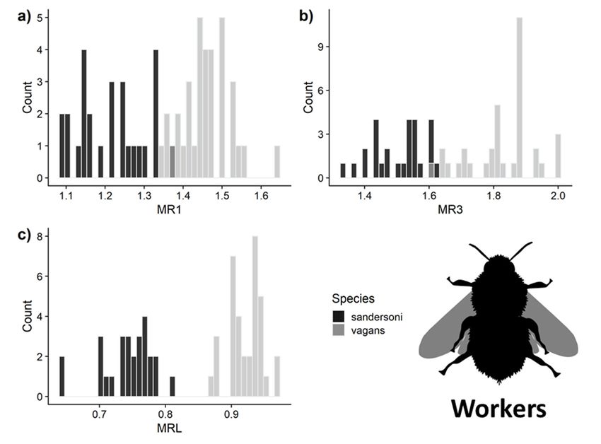
Insects 2020, 11, 669                                                                             3 of 20

structural character used to separate the queens of B. vagans from B. sandersoni. Mitchell [27] compared
the median length of the malar space in relation to the basal width of the mandible to differentiate the
spring-caught queens of B. sandersoni from B. vagans. Although these morphometric characters are
effective for distinguishing among spring-caught queens of B. sandersoni and B. vagans, none of these
authors used these characters to separate worker specimens of these species. Size polymorphism in
worker bumble bees can exhibit up to 10-fold variation in body mass within a single colony [35,36],
and visual assessment of the malar length of smaller bodied bees without the aid of a microscope
presents a greater challenge. This is important because workers are more abundant and active during
the flight season than queens, and thus more likely to be encountered by field investigators and
collected as specimens during community and population monitoring [37].
     Earlier authors did not provide quantitative comparisons for morphologic features in worker
castes, only in spring-caught queens. For example, Mitchell [27] described qualitative differences
between B. sandersoni and B. vagans with respect to the malar character as “slightly greater”, “slightly
shorter than”, or “nearly equal”, and Williams et al. [23] provide a similar qualitative assessment of
the cheek length to width to distinguish between these species. Richards [31], in his work on the
subgeneric divisions of Bombus Laterille, provided measurements of several morphometric characters
using a micrometer scale (reticle) to provide measurements as units including those for absolute
malar length and the proportions of antennal segments 3:4:5 in females, but he did not apply these
findings to species within the subgenera. Although the descriptive morphological features used by
previous authors provide a means for discriminating among these species, variability within species
may make accurate determinations based on these characteristics difficult and have not been tested in
workers [23,25].
     To assess conservation assessments for species of bumble bees, and to monitor population
status and trends, accurate identification is required. We undertook this study to establish reliable
quantitative morphometric characters to distinguish among B. sandersoni, B. vagans and B. perplexus,
using specimens of both queens and workers that were independently identified using DNA sequence
data. We predicted that if these characters were useful for discriminating among species, then
classifying species based on morphometrics would correspond to classifications based on DNA [37].
In addition, we assessed the accuracy of characters currently employed to separate these species,
compare measurement repeatability within and between observers, and provide guidelines for accurate
identification of this species complex for future studies.

2. Materials and Methods

2.1. Specimens
     Specimens of worker and spring and fall-caught queen B. vagans, B. sandersoni, and B. perplexus
were collected from 2010–2019 from the northern edge of their range in three states in the Midwest
(Minnesota, Wisconsin, and Michigan) and three states in the northeast (New York, Massachusetts,
and Maine) to represent regional diversity (see Supplemental Appendix A for complete specimen
collection information). Initial species identifications were made on 216 specimens using taxonomic
keys [23,27,38] and accompanying visual assessments of the ocular-malar area and hair color and
patterns on the thorax and tergal segments. We did not include males in our analysis because they can
be reliably identified using standard keys [23,27]. To confirm species identifications, we obtained DNA
sequence data on 115 specimens haphazardly chosen from the 216 specimens to include individuals
tentatively identified as one of the focal species based on visual observations, hair color pattern,
including the presence of yellow hair on tergal segment 5 (T%), and individuals whose species
assignment was not initially apparent (species information in Appendix A).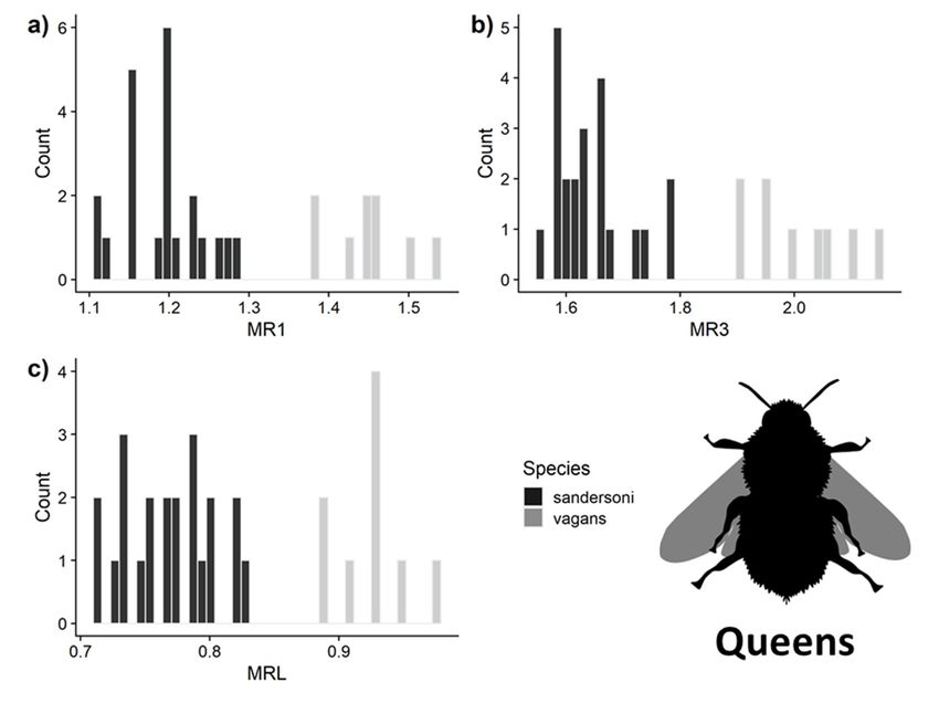
Insects 2020, 11, 669 4 of 20
Insects 2020, 11, x FOR PEER REVIEW 4 of 23
2.2. Determining
2.2. Determining Malar
Malar and
and Flagellar
Flagellar Segment
Segment Ratios
Ratios
Using aa reticle
Using reticle in
in the
the eyepiece
eyepiece of of aa stereomicroscope,
stereomicroscope, we we measured
measured thethe malar
malar length,
length, width,
width, and
and
length of flagellar segments 1 and 3 on 216 specimens, including the 115 (44 B. vagans,
length of flagellar segments 1 and 3 on 216 specimens, including the 115 (44 B. vagans, 49 B. sandersoni, 49 B. sandersoni,
and 22 B.
and 22 B. perplexus)
perplexus) that
that were
were subsequently
subsequently chosenchosen for
for DNA
DNA analysis. Following the
analysis. Following the anatomy
anatomy in in
Michener [39] and Williams et al. [23], we measured the malar length (i.e., the shortest
Michener [39] and Williams et al. [23], we measured the malar length (i.e., the shortest distance from distance from
the base
the base of
of the
the eye
eye to
to the
the edge
edge of
of the
the cheek
cheek (Figure
(Figure 1),
1), and
and the
the malar
malar width
width (i.e.,
(i.e., the
the outside
outside ofof the
the
mandible condyle
mandible condyle toto the
the outside
outside ofof the
the cheek
cheek condyle,
condyle, assumed
assumed to to be
be synonymous
synonymous with with the
the “basal
“basal
width
width of the mandible”
of the mandible” following
following Mitchell
Mitchell [27]
[27] (Figure
(Figure 1a)
1a) on queens and
on queens and workers
workers to to establish
establish aa range
range
of MRL length to width ratios. To ensure consistency of measurements, we
of MRL length to width ratios. To ensure consistency of measurements, we measured the malarmeasured the malar length
on bothon
length the vertical
both and horizontal
the vertical axis to confirm
and horizontal that ourthat
axis to confirm measurements were constant.
our measurements were constant.
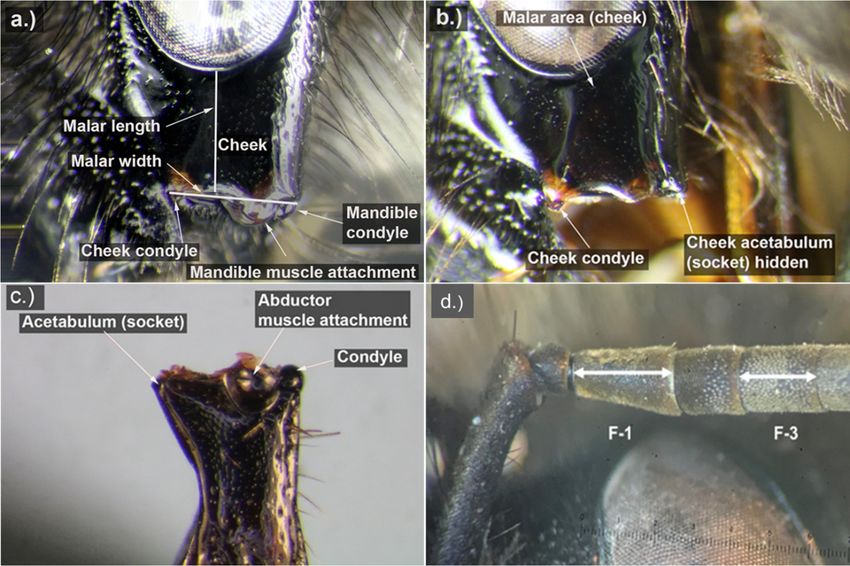
Figure
Figure 1.
1. Images
Images of
ofaafemale
femaleBombus
Bombusvagans
vaganscheek
cheekandandflagellar
flagellarsegments
segments illustrating
illustrating the
the measurement
measurement
locations for the malar length, malar width, and lengths of flagellar segments 1
locations for the malar length, malar width, and lengths of flagellar segments 1 and 3. (a) and 3. (a) Anatomy
Anatomy of
the cheek. (b) Simplified image of the cheek with the mandible removed to show
of the cheek. (b) Simplified image of the cheek with the mandible removed to show placement of placement of the
cheek condyle
the cheek and and
condyle cheek acetabulum.
cheek acetabulum.(c) Simplified image
(c) Simplified of the
image of anatomy
the anatomy of the
of mandible. (d)
the mandible.
Flagellar segments
(d) Flagellar 1 and
segments 3 illustrating
1 and where
3 illustrating wheretotomake
makemeasurements
measurementstotorecord
recordlength.
length. Photos
Photos a-c
a-c by
by
Dennis Johnson.
Dennis Johnson.
To take
take malar
malarwidth
widthmeasurements,
measurements,we weused
usedthethe cheek
cheek condyle
condyle to demark
to demark thethe medial
medial edgeedge of
of the
the mandible,
mandible, because
because whenwhen the mandible
the mandible of the specimen
of the specimen is closed,istheclosed, the small
small corner corner
of the of the
acetabulum
acetabulum
is hidden byisthe
hidden
lateralbyedge
the lateral edge of (Figure
of the clypeus the clypeus
1b,c).(Figure 1b,c).condyle
The cheek The cheek condyle
aligns with aligns with
the hidden
the
edgehidden
of theedge of the and
mandible mandible and marks
therefore therefore
themarks thethe
edge of edge of the mandible
mandible (Figure
(Figure 1b). The1b). Thelength
malar malar
length
to widthtoratio
width
is calculated as MRL =asmalar
ratio is calculated MRLlength/malar
= malar length/malar
width. Next,width. Next, we the
we measured measured the
horizontal
horizontal lengths ofsegments
lengths of flagellar flagellar 1segments 1 and 3.1d)
and 3. (Figure (Figure 1d) to establish
to establish a range ofa malar
range of malar
length tolength to
flagellar
flagellar length
length ratios for ratios forsegments
flagellar flagellar 1segments
(MR1) and 1 (MR1)
3 (MR3)and 3 (MR3)
using using the
the following followingMR1
calculations = malar
calculations
MR1
length/flagellomer − 1, and MR3− =1,malar
= malar length/flagellomer and MR3 = malar length/flagellomer
length/flagellomer − 3. Detailed − 3. Detailed instructions
instructions on how to
on how tothe
measure measure
MRL, MR1,the MRL, MR1,ratios
and MR3 and MR3 ratios areinprovided
are provided Appendix in B.
Appendix B.
To examine
examineany any possible
possible effects
effects fromfrom observer
observer biasesbiases and experiences,
and experiences, each specimen
each specimen was
was measured
measured by two independent
by two independent observers (Hereafter:
observers (Hereafter: Obs1 and
Obs1 and Obs2). Obs2). To determine
To determine the extent tothewhich
extentthis
to
which this methodology could be employed by a novice, specimens were measured by a student
volunteer with < two months of experience identifying bees under a microscope (Hereafter: Obs3).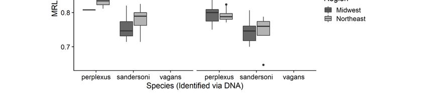
Insects 2020, 11, 669                                                                                 5 of 20

methodology could be employed by a novice, specimens were measured by a student volunteer with
< two months of experience identifying bees under a microscope (Hereafter: Obs3).

2.3. DNA Barcoding
      To provide species-level identifications to determine the accuracy of existing keys and our MRL,
MR1, and MR3 measurements, DNA was extracted from 115 specimens for which we had used existing
keys and made visual identifications. From each specimen, the central-right leg was removed using
sterilized forceps, legs were ground in a 1.5 mL microcentrifuge tube using a polypropylene pestle
(USA Scientific, Inc., Ocala, FL, USA) and whole genomic DNA was isolated using the Omega Bio-tek
E.Z.N.A.® Tissue DNA Kit (Omega Bio-tek, Inc., Norcross, GA, USA). After isolation, a fragment
of the mitochondrial locus cytochrome oxidase I (COI) was amplified using the protocol described
in Hebert et al. [40]. Initial attempts to amplify the complete “barcode” fragment using the primers
LepF1 and LepR1 as described in Hebert et al. [40], were unsuccessful, likely due to extractions that
were performed from pinned specimens of varying ages. Therefore, we designed novel primers
BombusF (50 -AGWCAYCCTGGAATATGAA-30 ) and BombusR (50 -GTGGRAAAGCTATATCAGG-30 )
to amplify ~150 base-pairs of the barcode fragment that was diagnostic among species. PCRs were
conducted following conditions described in Smith-Freedman et al. [41], and DNA sequencing of
both forward and reverse fragments was performed at the DNA Analysis Facility on Science Hill
at Yale University. Raw sequence reads were edited in Geneious 11.1.2 (Biomaters Ltd., Auckland,
New Zealand), and the forward and reverse reads assembled into a consensus sequence for each
sample, and an alignment of all sequenced samples was then constructed in Geneious using the
“Geneious Alignment Tool” with default parameters. Sequences were then assigned to haplotypes,
and the relationships of haplotypes to each other were reconstructed using TCS v. 1.21 [42] with a
95% connection limit. Inter- and intraspecific percent differences between and among each species
were then calculated in Geneious based on the species identifications from the TCS network analysis.
DNA barcodes associated with all specimens are accessible on GenBank under the Accession numbers
MT951454-MT951575, MT991562-MT991569 (Appendix A).

2.4. Statistical Analyses
      To determine the accuracy of visual identifications (i.e., traditional identifications which are based
on hair coloration and just visual observations of malar length) in comparison to DNA-confirmed
identifications we performed Pearson’s correlation tests. To compare mean malar ratio measurements
among the three species, we used a generalized linear model (GLM) that included the malar ratio
measurement as our response (either MR1, MR3 or MRL), a fixed effect of species (identified by
DNA barcoding), bee caste (queen or worker) and region (Midwest or Northeast). We also included
an interaction term between species and caste and between species and region. We ran this model
assuming a Gaussian error distribution and tested variable significance using analysis of variance
(ANOVA). Non-significant interaction terms (p > 0.05) were removed, and the analysis rerun with the
remaining fixed effects and interaction terms [43]. Pairwise differences among levels within our fixed
effects with least-squares means were compared using the package ‘emmeans’ to acquire estimated
means and Tukey-adjusted p-values [44].
      To test the accuracy of the three malar ratio measurements for identifying species, we used a
linear discriminant analysis (LDA) on queens and workers separately for B. sandersoni and B. vagans.
B. perplexus was excluded from this analysis because we found that hair color, even on the less common
light-colored specimens, contained a few scattered dark hairs on the thorax, and in most cases, light
form specimens had light hair on the third tergal segment. Thus, malar ratio measurements were
unnecessary for this statistical comparison. However, we present B. perplexus MRL, MR1, and MR3
ratio ranges to alert taxonomists to the possibility of rare, light-colored B. perplexus that may require
additional characters to confirm identification.
Insects 2020, 11, 669 6 of 20
We performed an LDA on 60% of our 115 DNA verified specimens to use as a training dataset
and then predicted species identification on the remaining 40% of samples using MR1, MR3, and MRL
measurements and validated the accuracy of our classifications using the species identifications from
the DNA barcodes. We ran the LDA using the function ‘lda’ in package ‘MASS’ [45] and split the
data using function ‘createDataPartition’ from package ‘caret’ [46]. To quantify the uncertainty in
accuracy using three measurements, we performed a bootstrapping method to resample the dataset
999 times and determined the median ± SD of accuracy for the three measurements for both queens
and workers separately.
We then predicted a range of values for each measurement beyond our measured individuals using
the sample mean and SE. For each species/caste combo (e.g., B. sandersoni queens), we first bootstrapped
the population mean and standard error by 500 sampled replicates using the function ‘boot’ from
package ‘boot’ [47]. We then simulated a population of 10,000 bees from a normal distribution using
the bootstrapped mean and SD and report the 99% quantile of the simulated distribution. All analyses
were performed using the statistical environment R v. 3.5.1 [48].
Finally, we assessed the repeatability of malar ratio measurements by different observers.
We compared measurements within and among observers using a Pearson’s correlation using the
function ‘cor,test’ in R [48]. We first compared measurements by experienced Obs1 to measurements
by both an experienced Ob2 and inexperienced Ob3. We also examined the correlation between
standard deviation (SD) and the mean of repeated measurements within and between observers to
determine if repeatability was associated with measurement size (e.g., observations become less reliable
as individuals decrease in size).
3. Results
3.1. Malar Ratio Measurements & DNA Barcoding
We collected measurements for MRL, MR1, and MR3 from a total of 216 specimens and obtained
DNA results from 115 specimens to confirm species identifications (49 B. sandersoni, 44 B. vagans,
22 B. perplexus). Without using quantified malar length to width or flagellar length ratios, our
identifications based on existing keys and visual characteristics (e.g., hair color) were correct 70.4% of
the time. For all worker and queens, the malar length was smaller than the malar width. Correlation
between the three malar ratio measurements were strong (MR1 to MR3:R = 0.66, MR1 to MRL R = 0.75,
MR3 to MRL:R = 0.77). For all species comparisons, we use measurements from only one observer
(Obs1) to avoid pseudoreplication.
Based on statistical parsimony reconstruction, individuals could be assigned to one of three groups
representing individuals of (1) B. sandersoni (haplotype MR001), (2) B. vagans (haplotype MR003),
and (3) B. perplexus (haplotypes MR191 and MR196 [one base-pair different between the two B. perplexus
haplotypes]). The relationship of each group is presented in Figure 2.
Mirroring the network analyses, estimates of intra- and interspecific percent differences, found
that individuals of B. sandersoni and B. vagans were 95.7% similar to each other (both species had
100% within species similarity), and that on average individuals of B. perplexus were 94.3% similar to
individuals of both B. sandersoni and B. vagans (this species had 99.3% within species similarity due to
the one-basepair difference between haplotype MR191 and MR196).
3.2. Comparing the Three Measurements among Species
For all three measurements, means were significantly different among the three species and
between queens and workers (Tables 1 and 2, Figure 3). However, differences between queens and
workers varied among measurements. Queens had larger MR3 and MRL measurements compared to
workers, but there was no difference in MR1 between queens and workers (Tables 1 and 2, Figure 3).
There were no significant differences in any measurement between the two geographic regions (Table 1)between the three malar ratio measurements were strong (MR1 to MR3:R = 0.66, MR1 to MRL R =
0.75, MR3 to MRL:R = 0.77). For all species comparisons, we use measurements from only one
observer (Obs1) to avoid pseudoreplication.
Based on statistical parsimony reconstruction, individuals could be assigned to 7one
Insects 2020, 11, 669 of 20
of three
groups representing individuals of (1) B. sandersoni (haplotype MR001), (2) B. vagans (haplotype
MR003), and (3) B. perplexus (haplotypes MR191 and MR196 [one base-pair different between the two
nor were there any significant interactions among species, castes, or region for any measurement
B. perplexus
(all p haplotypes]).
> 0.1). The relationship of each group is presented in Figure 2.
Key
Bombus vagans Wisconsin
New York
New Jersey
Minnesota
Michigan
Massachusetts
Maine
Bombus sandersoni
MR191
MR196
Bombus perplexus
Figure
Figure 2. 2. Statistical
Statistical parsimonynetwork
parsimony network highlighting the relationships
highlighting the relationships ourBombus
of our threeoffocal threespecies.
focal Bombus
For each species, charts are drawn proportional to the number of sequenced individuals, and colored
species. For each species, charts are drawn proportional to the number of sequenced individuals, and
according to the geographic region from which individuals were collected. White circles are drawn to
signify individual base pair differences between haplotypes.
Table 1. Results from generalized linear model (GLM), ANOVA and pairwise differences of fixed
effects comparing the measurement means among the three species and between castes and regions.
† Species comparisons are the Tukey’s HSD adjusted p-value.
Response Variable Levels β ± SE df F p†
2110 183.18Insects 2020, 11, 669 8 of 20
Table 2. Estimated means from the linear model for the three malar ratio measurements and among
the three species for both workers and queens. Results are averaged over the two levels of region.
MR1 MR3 MRL
Species Caste
(Mean ± SE, 95% CI) (Mean ± SE, 95% CI) (Mean ± SE, 95% CI)
Worker 1.40 ± 0.02, 1.37–1.42 1.63 ± 0.02, 1.59–1.67 0.80 ± 0.01, 0.78–0.81
perplexus
Queen 1.38 ± 0.02, 1.34–1.41 1.79 ± 0.03, 1.74–1.85 0.82 ± 0.01, 0.80–0.83
Worker 1.21 ± 0.01, 1.19–1.24 1.49 ± 0.02, 1.46–1.53 0.75 ± 0.01, 0.74–0.76
sandersoni
Queen 1.19 ± 0.01, 1.17–1.22 1.66 ± 0.02, 1.62–1.69 0.77 ± 0.01, 0.75–0.78
Insects 2020, 11, Worker
vagans 1.46 ± 0.01, 1.44–1.48
x FOR PEER REVIEW 1.83 ± 0.02, 1.80–1.86 0.92 ± 0.01, 0.91–0.93
8 of 23
Queen 1.44 ± 0.02, 1.41–1.47 2.00 ± 0.02, 1.95–2.04 0.94 ± 0.01, 0.93–0.96
Figure 3. Comparison of malar ratios among the three Bombus species, caste, and between the regions
Figure 3. Comparison of malar ratios among the three Bombus species, caste, and between the regions
for thefor
following measurements: (a) MR1, (b) MR3 and (c) MRL.
the following measurements: (a) MR1, (b) MR3 and (c) MRL.Insects 2020, 11, 669 9 of 20
3.3. Predictive Accuracy of the Three Measurements for Separating B. vagans and B. sandersoni
Insects 2020, 11, x FOR PEER REVIEW 9 of 23
Using the measurements of queens, the LDA model predicted species identity with 100% accuracy
3.3. Predictive Accuracy of the Three Measurements for Separating B. Vagans and B. Sandersoni
for all three malar ratio measurements (Figure 4). For workers, MRL had 100% ± 0% SD and MR1 had
Using the measurements of queens, the LDA model predicted species identity with 100%
96% ± 5% accuracy
SD accuracy, and MR3 had a 97% ± 4% SD accuracy (Figure 5). Only MRL had complete
for all three malar ratio measurements (Figure 4). For workers, MRL had 100% ± 0% SD and
separationMR1 between
had 96% B.± vagans and B. sandersoni
5% SD accuracy, and MR3 hadfor queens
a 97% ± 4% SDand workers.
accuracy However,
(Figure using
5). Only MRL hadboth MR1
and MR3 complete
measurements
separationtobetween
differentiate
B. vagansspecies resulted
and B. sandersoni forin ± 0.01%
99% and
queens SD
workers. accuracy.
However, usingWe report
both MR1
characteristics of theand MR3species
three measurements
and theto differentiate
min and max species resulted
of all in 99% ± 0.01%
measurements SD accuracy.
as well We quantile
as the 99%
report characteristics of the three species and the min and max of all measurements as well as the
of our simulated distributions (Table 3).
99% quantile of our simulated distributions (Table 3).
Figure 4. Distribution of malar
Figure 4. Distribution ratioratio
of malar measurements
measurements ofofqueens
queens used
used inlinear
in the the linear discriminant
discriminant analysis analysis
(LDA) for (a) malar
(LDA) for length to flagellar
(a) malar length to segments 1 (MR1),
flagellar segments 1 (b) MR3
(MR1), (b)and
MR3 (c)and
MRL.(c) All
MRL.three
All measurements
three
had 100% measurements
accuracy for had 100% accuracy
predicting species foridentities
predicting on
species identities on
subsampled subsampled
datasets. datasets.
Image from Image
phylopic.org.
Insects 2020, 11, x FOR PEER REVIEW 10 of 23
from phylopic.org.
Figure 5. Distribution
Figure 5. Distribution of malar
of malar ratioratio measurements of
measurements ofworkers
workersused in the
used inLDA
the for
LDA (a) MR1, (b)MR1,
for (a) MR3 (b) MR3
and (c) MRL. Measurement accuracy ranged from 95–100%. Image from phylopic.org.
and (c) MRL. Measurement accuracy ranged from 95–100%. Image from phylopic.org.Insects 2020, 11, 669 10 of 20
Table 3. Characteristics, observed, and predicted measurement ranges † for the three Bombus species in this study.
Mesipisternum Presence of Black Presence of Yellow
Species Caste N MR1 † MR3 † MRL †
Hair Color Hairs on Scutum Hairs on T5
1.29–1.53 1.40–1.78 0.75–0.85
perplexus Worker 19 dark-light none-few none-few
(1.24–1.56) (1.37–1.86) (0.73–0.85)
1.10–1.37 1.33–1.63 0.65–0.81
sandersoni Worker 27 light few-many none-few-many
(1.00–1.42) (1.30–1.70) (0.64–0.84)
1.35-1.65 1.60–2.00 0.87–0.97
vagans Worker 35 light many none-few-many
(1.30–1.62) (1.57–2.08) (0.86–0.99)
1.36-1.39 1.67–2.00 0.81–0.86
perplexus Queen 3 dark none-few none
(1.35–1.40) (1.54–2.20) (0.78–0.87)
1.11–1.28 1.56–1.79 0.71–0.83
sandersoni Queen 22 light few-many none-few-many
(1.07–1.31) (1.48–1.81) (0.68–0.85)
1.38–1.54 1.90–2.15 0.89–0.98
vagans Queen 9 light many none-few-many
(1.33–1.57) (1.80–2.22) (0.86–0.99)
† Minimum and maximum values taken from Observer 1. Values inside parentheses are the estimated 99% quantile from the bootstrapped mean.Insects 2020, 11, 669 11 of 20
3.4. Correlation within and between All Observers
Repeat measurements of MR1, MR3, and MRL were highly correlated within observers, as
were measurements between both experienced observers (R > 0.9, Table 4). Correlations between
experienced and inexperienced observers were also strong but slightly lower than ratios measured by
experienced observers (R = 0.81compared to 0.85, Table 4). The standard deviation of measurements
was small (range: 0 to 0.11), and for MR1 and MR3 there was no evidence of a relationship between the
standard deviation of measurements and the mean in either measurement for both experienced and
inexperienced observers (Table 4). There was a weak tendency for SD to decrease as mean increased
for MRL (R-0.18, Table 4), suggesting this measurement may be more difficult to measure accurately
when specimens are small.
Table 4. Correlations between replicate measurements within and between experienced and
inexperienced observers. Inexperienced Obs3 did not make MRL measurements therefore comparisons
are not included here.
Comparison Measurement R t df p
MR1 0.95 33.08 113Insects 2020, 11, 669 12 of 20
always have T5 black except in specimens collected in Newfoundland. In our specimens, the presence
of yellow hairs on T5 was found in specimens collected in four different states in both the Midwest
and Northeast regions of the United States. Further complicating hair color as a useful identification
tool is preparation quality, such that hair color is often difficult to distinguish in Bombus specimens
with matted hair, a not uncommon state of some Bombus specimens in collections. We found that
B. perplexus can usually be identified by some of the following hair color patterns (1) the scutum has
all light hair, or rarely with a few black hairs whereas B. vagans and B. sandersoni usually have many
black hairs in this area, (2) the lower half of the pleura usually has dark hairs (common dark form),
which the other two species do not, (3) the uncommon “light form” appears to have no dark hairs on
the pleura, although often a few can be found low down around the legs, and (4) light form B. perplexus
often have some yellow hairs on T3 which would not be the case for the other two species. While hair
color can be useful to identify most B. perplexus, careful examination of malar ratio measurements
is essential to confirm identification of light-form B. perplexus, and in some challenging cases, DNA
confirmation may still be necessary. Additionally, while the malar ratios we present were calculated
based on the examination of physical specimens of workers and queens, it is possible that they could be
integrated into future community science projects (also called ‘citizen science’) if detailed photographs
of the malar region and flagellar segments were taken providing a clear image that could be digitally
measured with our methods.
The morphological similarity among these three species highlights the inherent challenges to
accuracy in community science projects that do not collect specimens. Goulson et al. [49] point out that
community science surveys are often limited by the taxonomic skills of the observers, particularly for
bee species that are difficult or impossible to identify in the field because of cryptic coloration. MacPhail
et al. [50] reported that 46.3% of B. vagans, 38.6% of B. sandersoni, and 86.4% of B. perplexus were correctly
identified from photos of Bombus by project designated expert taxonomists, or they were placed into a
“two-striped species group” when the photos were ambiguous. Richardson et al. [13] found that they
could reliably make a species determination from 68% of photographs submitted by participants in the
Vermont Bumble Bee Atlas. Suzuki et al. [51] in their survey of bumble bees in Japan found that they
had high consistency of identification from photos that ranged from 95–97.7%. The higher success rate
in Japan could be contributed to fewer species that exhibited similar hair patterns. However, none of
these identifications were validated with DNA sequence data. For our three focal species with similar
hair coloration, the use of photographs alone as a means for identification represents a cautionary tale.
Prior to this study, there were no established quantitative morphometric measurements ranges
for workers of these three species. In his comprehensive paper “The Bombidae of the New World,”
Franklin [25], included a chart of the range of malar spaces for spring-caught queen B. vagans, as lengths
vs. the widths of the eye expressed in Filar micrometer spaces (divisions) and expressed them as ratios.
Using spring-caught queen B. sandersoni and B. vagans, Plowright and Pallett [28] presented their
results for the means and range lengths of malar spaces and the length of the malar space-to-length of
the 3rd antennal segment. If we assume that their antennal segment three is equivalent to our flagellar
segment 1, then their measurements were similar to our results for queen B. vagans but showed greater
variation for queen B. sandersoni. There is some ambiguity in their results because the authors did not
provide detailed instruction on where they made their malar and flagellar measurements, nor did they
validate their specimen identifications using DNA sequence data. Based on our measurements for MRL,
MR1, and MR3, and our DNA confirmed species identification, we have been able to provide a reliable
range of values to differentiate B. vagans and B. sandersoni. However, and perhaps not unexpected
given its name, our values for B. perplexus overlapped the other two species, though generally accurate
identifications can be made based on observations of hair coloration combined with malar ratios.
Although the three species we discuss in this paper are considered species of least conservation
concern by ICUN criteria at this time [52], we recognize that bumble bees that were once
considered common can experience rapid declines in population size and range restrictions as
witnessed in Bombus affinis Cresson, B. terricola Kirby, and B. pensylvanica Degeer; species nowInsects 2020, 11, 669 13 of 20
considered Critically Endangered or vulnerable by the IUCN SSC Bumblebee Specialist Group
(https://bumblebeespecialistgroup.org/north-america/). Moreover, population status for B. vagans
and B. sandersoni varies considerably over different regions. For example, Jacobson et al. [11] found
a significant decline in B. vagans in New Hampshire over the past 150 years. Similarly, B. vagans
was considered to be in decline in Canada in 2008, but then deemed stable in 2012 because of an
increase in records despite a reduction in historical range size [7,53] and was considered a candidate for
additional monitoring [54]. In Illinois, Grixti et al. [55] report that B. vagans was locally extirpated from
its historic southern and northern ranges. In a review of historical changes in US bees with shared
ecological traits, Bartomous et al. [5] found that B. vagans exhibited a decline but that B. sandersoni
was stable. Franklin [56] considered B. sandersoni to be one of the most abundant species in its
range, but it was rare in New Hampshire [11], and in Canada it was considered a candidate for
immediate conservation concern [52] despite its status of Least Concern on the ICUN Red List [53].
Similarly, Richardson et al. [13] noted a 53% decline in B. sandersoni although a 266% increase in
B. vagans abundance in in Vermont. B. perplexus appears to be increasing overall in abundance in the
US and Canada [5,53]. Goldstein and Ascher [57] suspected that B. sandersoni may be under-reported
on Martha’s Vineyard, MA because of its similar coloration with B. vagans, and to lesser degree,
B. perplexus. Thus, conflicting reports of population trends in these cryptic species could be due in part
to misclassification of specimens due to limitations in the diagnostic characteristics that were used
to identify these species. This highlights our argument that accurate identifications are essential to
accurately track population status and trends consistently across regions.
5. Conclusions
Around the globe, efforts are currently underway to examine changes in the distributions
and abundance of pollinator species [17,58–60], with particular focus on the status of the native
species [7,52,61–64]. However, for country and state-wide monitoring programs, or large-scale
community science programs such as Bumble Bee Watch (https://www.bumblebeewatch.org/) and
their associated conservation projects, providing accurate information on bumble bee population
size and distribution depends on reliable identifications. The methods we present allow researchers
to accurately discriminate among queens and workers of three cryptic species of bumble bee that
had formerly posed a challenge to identify, particularly in worker specimens. The standardization
of the MRL, MR1, and MR3 methods as we have defined them, and the range of values for each of
the three species, provides an important tool to reliably identify species beyond visual characters
such as hair coloration for B. perplexus and assessments of malar length in B. vagans and B. sandersoni.
DNA analysis is an excellent tool to provide species identifications [65], but not everyone has access
to DNA facilities or funding. In addition, care needs to be taken when interpreting DNA analyses
(particularly for DNA barcoding projects) as results can often be misleading due to factors such as
(but not limited to) the unintended amplification of non-target organisms (e.g., parasites, parasitoids,
endosymbionts, etc.), the amplification of non-target loci (e.g., nuclear copies of mitochondrial DNA),
and misidentifications in public databases (e.g., BOLD or GenBank). We are encouraged that the
combination of DNA sequencing and morphological measurements was able to illuminate characters
that can be used to accurately identify members of this confusing group of bumble bees, and we hope
that as new technologies (such as Next-Generation sequencing) allow for high-throughput analyses
of communities of organisms, that similar synergistic studies will be performed in other groups as
well. The measurements we provide here to determine MRL, MR1, and MR3 values for B. sandersoni,
B. vagans, and B. perplexus can be done with a minimum investment in equipment and time and
provides highly accurate identification outcomes of these cryptic species required to inform effective
monitoring and management decisions.
Author Contributions: Conceptualization, D.E.J., J.M.; Methodology, J.M., D.E.J.; Investigation, J.M., D.E.J.,
A.B.F., J.C.A.; Validation, J.M., A.B.F., D.E.J.; Formal Analysis, D.L.N., J.C.A.; Resources, J.M., J.S.E., J.C.A.,
DIN.; Writing—Original Draft Preparation, J.M.; Writing—Review & Editing, J.C.A., D.L.N., A.B.F., J.S.E., D.E.J.;Insects 2020, 11, 669 14 of 20
Supervision, J.M., Project Administration, J.M., A.B.F.; Visualization: D.L.N., D.E.J., J.M.; Funding Acquisition
J.S.E. All authors have read and agreed to the published version of the manuscript.
Funding: Funding for this project was provided by J.S.E. (Research Trust Funds).
Acknowledgments: We are grateful to the U.S. Forest Service Eastern Region, the Chequamegon Nicolet, Finger
Lakes, Hiawatha, Huron Manistee, Ottawa and Superior National Forests, and Chris Buelow of the Massachusetts
Division of Fisheries and Wildlife, for allowing us to measure bee specimens collected on their property to use in
our analyses. Thank you to Dave King, Michael Veit, and three anonymous reviewers for their comments on a
previous version of this manuscript, and to Sam Droege for his encouragement and testing of this approach in its
early form.
Conflicts of Interest: The authors declare no conflict of interest.
Ethics Approval: The authors declare that there is no conflict of ethics.
Consent to Participate: (NA).
Consent for Publication: (NA).
Availability of Data and Material: Limited data presented in the manuscript; complete data and specimens
available upon request.
Code Availability: Not applicable.
Data Deposition: Specimen and genetic data reported in this paper are included in Appendix A.
Appendix A
Table A1. Project bumble bee specimens for determining ratios of MRL, MR1, and MR3 presented
by project number, caste, collection date, collection state, latitude, longitude, verified DNA results,
and GenBank Accession numbers.
GenBank
Project ID Coll. Date State DNA
Caste Latitude Longitude Accession
Number m/d/yr. Collected Results
Numbers
MR_003 w 8/23/2018 WI 45.1385 −88.4728 vagans MT951529
MR_004 w 7/25/2018 WI 45.2704 −88.3468 vagans MT951530
MR_076 w 7/23/2018 WI 45.2002 −88.5869 vagans MT951532
MR_077 w 7/26/2018 WI 45.2996 −88.3899 vagans MT951533
MR_079 w 7/26/2018 WI 45.2996 −88.3899 vagans MT951534
MR_080 w 7/23/2018 WI 45.2002 −88.5869 vagans MT951535
MR_082 w 7/18/2018 WI 45.1682 −88.3119 vagans MT951536
MR_084 w 7/9/2018 WI 45.3415 −88.4195 vagans MT951537
MR_085 w 7/9/2018 WI 45.3198 −88.4079 vagans MT951538
MR_091 w 7/23/2018 WI 45.3199 −88.4072 vagans MT951539
MR_092 w 7/23/2018 WI 45.3199 −88.4072 vagans MT951540
MR_094 w 7/18/2018 WI 45.1682 −88.3119 vagans MT951541
MR_097 Q 6/8/2018 MI 46.5008 −90.0185 vagans MT951542
MR_102 w 6/26/2014 NY 43.7356 −73.8508 vagans MT951543
MR_105 w 8/15/2018 MI 46.5365 −89.0134 vagans MT951544
MR_118 Q 7/25/2018 WI 45.2704 −88.3468 vagans MT991562
MR_119 Q 8/30/2018 WI 45.9942 −88.4572 vagans MT991563
MR_121 w 8/14/2018 MN 47.7686 −90.8927 vagans MT951545
MR_124 w 7/25/2018 WI 45.2704 −88.3468 vagans MT951546
MR_127 w 8/15/2018 MI 46.5759 −88.8877 vagans MT951547
MR_133 w 8/14/2018 MN 47.7856 −90.8823 vagans MT951548
MR_134 w 8/14/2018 MN 47.7856 −90.8823 vagans MT951549
MR_136 w 8/14/2018 MN 47.7856 −90.8823 vagans MT951550
MR_144 w 7/19/2018 MA 42.6806 −72.1117 vagans MT951551
MR_146 w 7/18/2018 MA 42.6614 −72.1083 vagans MT951552
MR_151 w 7/10/2018 MN 47.7697 −90.3107 vagans MT951553
MR_154 w 7/2/2018 MN 47.4935 −91.9518 vagans MT951554Insects 2020, 11, 669 15 of 20
Table A1. Cont.
GenBank
Project ID Coll. Date State DNA
Caste Latitude Longitude Accession
Number m/d/yr. Collected Results
Numbers
MR_160 w 8/14/2018 MN 47.7686 −90.8927 vagans MT951555
MR_165 w 8/14/2018 MN 47.7686 −90.8927 vagans MT951556
MR_167 Q 7/23/2018 WI 45.2719 −88.6892 vagans MT991564
MR_168 w 7/18/2018 WI 45.1682 −88.3119 vagans MT951557
MR_180 w 7/11/2014 MA 42.5312 −72.3220 vagans MT951558
MR_184 w 8/22/2018 WI 45.3215 −88.4050 vagans MT951559
MR_185 Q 5/15/2018 WI 45.3215 −88.4050 vagans MT951560
MR_186 w 8/8/2018 WI 46.0250 −88.8744 vagans MT951561
MR_187 w 8/8/2018 WI 46.0250 −88.8744 vagans MT951562
MR_199 Q 7/10/2018 WI 45.1690 −88.3338 vagans MT991565
MR_200 Q 7/10/2018 WI 45.1690 −88.3338 vagans MT991567
MR_204 w 8/7/2018 WI 45.8141 −88.6540 vagans MT951563
MR_207 w 7/19/2018 WI 45.2951 −88.5143 vagans MT951564
MR_212 w 8/21/2018 MI 46.3424 −89.4668 vagans MT951565
MR_215 Q 7/10/2018 WI 45.1690 −88.3338 vagans MT951566
MR_219 w 7/10/2015 MA 42.5225 −72.3233 vagans MT951567
MR_220 Q 5/25/2014 ME 43.8978 −69.7676 vagans MT991566
MR_001 w 7/11/2018 MA 42.3481 −72.2324 sandersoni MT951476
MR_011 w 7/11/2018 MA 42.3481 −72.2324 sandersoni MT951477
MR_013 w 7/11/2018 MA 42.3466 −72.2272 sandersoni MT951478
MR_015 w 7/11/2018 MA 42.3446 −72.2275 sandersoni MT951479
MR_017 w 7/11/2018 MA 42.3481 −72.2324 sandersoni MT951480
MR_040 w 6/5/2018 MN 47.8405 −90.7564 sandersoni MT951483
MR_042 w 6/8/2018 MN 47.5978 −90.8237 sandersoni MT951484
MR_043 Q 6/5/2018 MN 47.7689 −90.8913 sandersoni MT951485
MR_047 w 7/9/2018 MN 47.5977 −90.8242 sandersoni MT951486
MR_048 w 7/10/2018 MN 47.7697 −90.3107 sandersoni MT951487
MR_052 w 7/9/2018 MN 47.5977 −90.8242 sandersoni MT951488
MR_053 w 7/2/2018 MN 47.4935 −91.9518 sandersoni MT951489
MR_055 w 7/9/2018 MN 47.5977 −90.8242 sandersoni MT951490
MR_057 w 7/9/2018 MN 47.5977 −90.8242 sandersoni MT951491
MR_058 w 7/9/2018 MN 47.5977 −90.8242 sandersoni MT951492
MR_060 w 7/10/2018 MN 47.7697 −90.3107 sandersoni MT951493
MR_061 w 7/10/2018 MN 47.7697 −90.3107 sandersoni MT951494
MR_062 w 7/10/2018 MN 47.7697 −90.3107 sandersoni MT951495
MR_065 w 7/10/2018 MN 47.7697 −90.3107 sandersoni MT951496
MR_067 Q 8/13/2018 MN 47.5977 −90.8242 sandersoni MT951497
MR_087 w 7/17/2014 MA 42.5020 −72.3690 sandersoni MT951499
MR_088 Q 5/6/2014 MA 42.4310 −72.2500 sandersoni MT951500
MR_095 Q 7/23/2018 MI 46.2213 −86.6676 sandersoni MT951501
MR_099 Q 5/23/2018 MN 48.0534 −90.0562 sandersoni MT951503
MR_103 w 6/9/2010 ME 44.3000 −68.3500 sandersoni MT951504
MR_108 Q 5/5/2014 MA 42.4182 −72.2535 sandersoni MT951505
MR_109 Q 5/5/2014 MA 42.4187 −72.2439 sandersoni MT951506
MR_113 Q 5/5/2014 MA 42.4312 −72.2501 sandersoni MT951507
MR_139 Q 6/12/2018 MA 42.3426 −72.2357 sandersoni MT951508
MR_142 Q 7/11/2018 MA 42.3504 −72.2274 sandersoni MT951509
MR_143 w 7/18/2018 MA 42.6590 −72.1068 sandersoni MT951510
MR_178 Q 5/5/2014 MA 42.4141 −72.2546 sandersoni MT951511
MR_179 Q 5/5/2014 MA 42.4141 −72.2546 sandersoni MT951512
MR_181 w 7/9/2014 MA 42.4407 −72.2490 sandersoni MT951513
MR_214 w 6/20/2018 MI 46.3424 −89.4668 sandersoni MT951514
MR_216 Q 5/6/2015 MA 42.4187 −72.2439 sandersoni MT951515
MR_217 w 7/6/2015 MA 42.4188 −72.2438 sandersoni MT951516
MR_218 w 7/16/2015 MA 42.5225 −72.3233 sandersoni MT951517Insects 2020, 11, 669 16 of 20
Table A1. Cont.
GenBank
Project ID Coll. Date State DNA
Caste Latitude Longitude Accession
Number m/d/yr. Collected Results
Numbers
MR_221 Q 5/3/2015 MA 42.5005 −72.2691 sandersoni MT951518
MR_224 w 6/20/2018 MI 46.3424 −89.4668 sandersoni MT951519
MR_225 w 6/6/2017 MN 47.7964 −90.9315 sandersoni MT951520
MR_229 Q 5/2/2015 MA 42.5312 −72.3219 sandersoni MT951521
MR_231 w 6/6/2017 WI 47.7660 −88.9701 sandersoni MT951522
MR_232 w 6/5/2017 WI 45.7384 −88.5829 sandersoni MT951523
MR_235 Q 5/2/2015 MA 42.5022 −72.3697 sandersoni MT951524
MR_237 Q 6/2/2018 WI 45.1311 −88.3738 sandersoni MT991568
MR_238 Q 6/6/2017 MN 47.2935 −91.9503 sandersoni MT951525
MR_239 Q 6/6/2017 MN 47.2935 −91.9503 sandersoni MT951526
MR_241 Q 6/6/2017 MN 47.2935 −91.9503 sandersoni MT951527
MR_009 w 6/20/2018 WI 45.9363 −88.9506 perplexus MT951454
MR_039 w 6/7/2017 MI 44.1351 −85.9340 perplexus MT951455
MR_050 w 8/23/2018 WI 45.1385 −88.4728 perplexus MT951456
MR_071 w 8/13/2018 MN 47.7856 −90.8823 perplexus MT951457
MR_115 w 5/24/2012 MA 42.3063 −72.6946 perplexus MT951458
MR_117 w 5/24/2012 MA 42.3063 −72.6946 perplexus MT951459
MR_130 w 6/20/2018 WI 45.9363 −88.9506 perplexus MT951460
MR_189 w 6/20/2018 WI 45.9363 −88.9506 perplexus MT951461
MR_190 w 8/13/2018 MN 47.7695 −90.3098 perplexus MT951462
MR_191 w 8/8/2018 MI 46.2715 −89.4930 perplexus MT951463
MR_192 w 8/8/2018 MI 46.2715 −89.4930 perplexus MT951464
MR_193 w 6/5/2018 MN 47.7689 −90.8913 perplexus MT951465
MR_194 Q 8/18/2018 MI 46.19618 −89.1594 perplexus MT951466
MR_195 w 8/15/2017 MI 46.3375 −89.4753 perplexus MT951467
MR_197 w 7/11/2018 MA 42.3399 −72.2330 perplexus MT951469
MR_198 w 7/16/2015 MA 42.4940 −72.2706 perplexus MT951470
MR_247 w 7/1/2019 MA 42.5824 −72.5301 perplexus MT951471
MR_248 w 7/3/2019 MA 42.5824 −72.5301 perplexus MT951472
MR_249 w 7/3/2019 MA 42.5824 −72.5301 perplexus MT951473
MR_250 w 7/3/2019 MA 42.5824 −72.5301 perplexus MT951474
MR_251 Q 7/3/2019 MA 42.5824 −72.5301 perplexus MT951475
MR_255 Q 4/25/2019 MA 42.3928 −72.5309 perplexus MT991569
Appendix B
Directions on how to measure the malar length and width (MRL) (technique developed by Dennis
E. Johnson), and how to measure the lengths of flagellar segments 1 and 3 to find MR1, and MR3 ratios
adapted from Plowright and Pallett (1978).
Appendix B.1. Equipment Required
1. A stereo microscope, preferably with a 45–50× zoom capability.
2. A 10× eyepiece with a reticle for measuring with at least one axis with 100 divisions in increments
of 10 is preferred but other reticles work as long as the scale is large enough to measure the malar
length and width.
3. Reticles can be acquired for most, but not all, microscope eyepieces. Reticles regularly require a
diopter adjustment to focus the reticle properly to ensure that the image of the reticle divisions are
sharp and clear. It is helpful to first perform this focus exercise on the microscope stage without a
specimen. The diopter adjustment compensates for differences between the observers’ eyes so it
should be re-adjusted for each user to compensate for variability among observers. Instructions
for diopter adjustments can be found online for microscopes and binoculars.Insects 2020, 11, 669 17 of 20
4. Specimens must be oriented so that the body part being measured is oriented perpendicular
to the axis of observation (e.g, place the specimen in a flat, horizontal position). A specimen
manipulator allows for a pinned specimen to be viewed from multiple angles while remaining
in a central viewing area under the microscope while allowing the viewer to maintain relative
focus while twisting or turning a specimen to show all sides. A large cork can also be used, but it
requires more patience to properly orient the specimen for measurement on a flat plane.
5. To make the measurements, either rotate eyepiece to orient the reticle in a horizontal or vertical
position or move the specimen. Try both methods to see which works best. Make one or more
measurements to confirm that they are the same value.
6. It is extremely important not to change the zoom between measurements. The specimen can be
moved, and the focus can be adjusted between the length and width measurements, but do not
change the zoom power. Each time you zoom up or down in power, the actual magnification
level may be slightly different. Changing the zoom level between measurements means that you
risk making your measurements at different magnification levels and the resulting ratios will be
incorrect. The power of the zoom used for making measurements is not important as long as
both measurements are made at the same magnification.
7. Take care to ensure that both ends of the of the body part to be measured are in focus.
8. Good lighting is important in making accurate determinations. A cool white LED ring lamp
works well.
9. Be careful to make sure that you are not 5 or 10 divisions off when reading the reticle measurement.
This is a common error.
Appendix B.2. How to Measure the MRL (Malar Length to Width)
1. Two measurements must be made to determine the malar ratio (MRL), i.e., the malar length and
the malar width as shown in Figure 1a. The measurements of the malar length and width are
made with the reticle and recorded as the number of reticle divisions. The malar length to width
ratio is calculated using the following equation.
MRL = malar length/malar width
2. Partial divisions are not estimated, rather the measurement is taken as the number closest to
the endpoint.
3. The malar length is measured as the shortest distance from the base of the eye to the edge
of the cheek using the definition from Williams et.al. [23]. The malar width is defined as the
measurement from the outside of the mandible condyle to the outside of the cheek condyle
(Figure 1a). This is equivalent to “cheek breadth” [23] or to the “basal width of the mandible” in
Mitchell [27]. See Figure 1b,c for separate views of the cheek and mandible.
4. Running a pin tip along the bottom edge of the cheek (away from the eye) helps to locate the
bottom end point to make the measurement.
5. We suggest measuring the length of the mandible at least twice, once on the horizontal axis and
again on the vertical axis, to ensure that these values are equal.
Appendix B.3. How to Measure the MR1 and MR3 (Malar Length to Flagellar Segment 1 and Malar Length to
Flagellar Segment 3 Length)
1. Measure the malar length as described above for MRL measurements.
2. Measure the length of flagellomer-1 along the horizontal axis. Place the zero end of the reticle
where the textured part of the segment begins (Figure 1d).
3. Measure flagellomer-3 on the horizontal axis (Figure 1d).You can also read