Virtual water trade and water footprint of agricultural goods: the 1961-2016 CWASI database
←
→
Page content transcription
If your browser does not render page correctly, please read the page content below
Earth Syst. Sci. Data, 13, 2025–2051, 2021
https://doi.org/10.5194/essd-13-2025-2021
© Author(s) 2021. This work is distributed under
the Creative Commons Attribution 4.0 License.

           Virtual water trade and water footprint of agricultural
                  goods: the 1961–2016 CWASI database
                           Stefania Tamea, Marta Tuninetti, Irene Soligno, and Francesco Laio
         Department of Environment, Land and Infrastructure Engineering, Politecnico di Torino, Turin, 10129, Italy
        Correspondence: Stefania Tamea (stefania.tamea@polito.it) and Marta Tuninetti (marta.tuninetti@polito.it)

                                  Received: 7 August 2020 – Discussion started: 6 November 2020
                         Revised: 20 February 2021 – Accepted: 24 February 2021 – Published: 12 May 2021

       Abstract. To support national and global assessments of water use in agriculture, we build a comprehensive
       database of country-specific water footprint and virtual water trade (VWT) data for 370 agricultural goods. The
       water footprint, indicating the water needed for the production of a good including rainwater and water from
       surface water and groundwater bodies, is expressed as a volume per unit weight of the good (or unit water foot-
       print, uWF) and is here estimated at the country scale for every year in the period 1961–2016. The uWF is also
       differentiated, where possible, between production and supply, referring to local production and to a weighted
       mean of local production and import, respectively. The VWT data, representing the amount of water needed for
       the production of a good and virtually exchanged with the international trade, are provided for each commodity
       as bilateral trade matrices, between origin and destination countries, for every year in the period 1986–2016.
       The database, developed within the CWASI project, improves upon earlier datasets because it takes into account
       the annual variability of the uWF of crops, it accounts for both produced and imported goods in the definition
       of the supply-side uWF, and it traces goods across the international trade up to the origin of goods’ production.
       The CWASI database is available on the Zenodo repository at https://doi.org/10.5281/zenodo.4606794 (Tamea
       et al., 2020), and it welcomes contributions and improvements from the research community to enable analyses
       specifically accounting for the temporal evolution of the uWF.

1   Introduction                                                   for volumes per unit weight; “crop water footprint” which ex-
                                                                   cludes livestock products; or “virtual water content” mainly
There has been a booming interest in the concept of wa-            used within the context of trade (see, e.g., Hoekstra et al.,
ter footprint (WF) since its introduction about 15 years ago       2011; Konar et al., 2011; Dalin et al., 2012; Tuninetti et al.,
(Hoekstra and Chapagain, 2007, 2008). The water footprint          2015). Also, the concept of virtual water, originally proposed
offers a common approach, language, and method to a wide           by J. A. Allan (1998) and from which the WF originated, has
range of analyses and multidisciplinary studies, and it is ap-     been growing in popularity among both the scientific com-
preciated for its capability to convey environmental messages      munity and the general public. Virtual water is the volume of
to the public. The WF identifies the freshwater needed for         water needed to produce a certain good that is virtually traded
the production of goods along the full supply chain, separat-      as a factor of production when the good is exchanged among
ing rainfall and water from surface water/groundwater bod-         countries. Such virtual flow defines the international virtual
ies. The WF assessment provides a quantitative framework to        water trade (VWT) and represents a metric that is suitable
analyze the volume of water embedded in agricultural goods         to analyze environmental aspects related to the global trade
and the efficiency of water use, when the metric is computed       of agricultural goods, to the water management and to the
per unit weight of the good (hereafter referred to as the unit     agricultural policy.
water footprint, or uWF). The term unit water footprint is            Assessment of WF and VWT requires a relatively large
here introduced to unify the current terminology which in-         amount of data, including production and trade data (in met-
cludes “water footprint”, used indifferently for volumes and

Published by Copernicus Publications.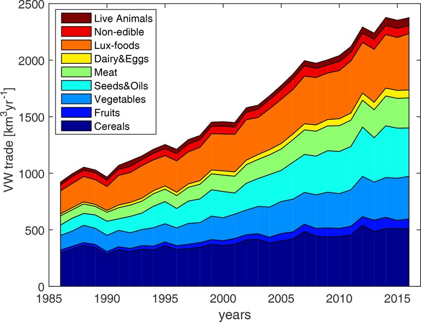
2026                                                                             S. Tamea et al.: 1961–2016 CWASI database

ric tons, t) and unit water footprint data (in m3 t−1 ). The        duction processes and associated water volumes. Within such
first remarkable database of uWF data has been prepared             an approach, the uWF of each good is multiplied by the (pro-
and shared by the Water Footprint Network, which pub-               duced or traded) quantity of the good, and resulting water
lished a large open-access dataset of uWF for several primary       volumes are then summed across goods. WaterStat is the
and processed agricultural goods, of crop and animal origin         main example of a bottom-up approach The top-down ap-
(Mekonnen and Hoekstra, 2010a, b). This database, named             proach aims at tracing full supply chains throughout eco-
WaterStat, includes average values over the period 1996–            nomic sectors and different countries. Input–output analyses,
2005 and has been the basis of the water footprint assess-          frequently used in economics for environmental assessments,
ment as presented, e.g., in Hoekstra et al. (2011). Other uWF       belong to this approach (Duarte and Yang, 2011). Bottom-up
datasets exist, which are based on spatially distributed mod-       approaches do not consider the entire supply chain of goods
els coupling the soil water balance with vegetation growth          and can be affected by truncation errors when used to assess
(see, e.g., Tuninetti et al., 2015, and references therein); such   the water footprint of final consumption (Feng et al., 2011).
databases mostly refer to a single year or a period or to long-     At the same time, bottom-up techniques can offer high com-
term averages. Other datasets, referring to blue water or to        modity resolution considering the water associated with the
scarcity-weighted indicators, are also available from the lit-      production of a large variety of single (agricultural) prod-
erature related to the life cycle assessment (e.g., Pfister et      ucts. A major problem affecting bottom-up approaches is
al., 2011, 2016). The temporal variability of uWF has been          the identification of the geographic origin of produced goods
seldom considered. Few examples include water scarcity in-          (Hubacek and Feng, 2016). In many cases, product re-export
dexes (e.g., Pfister and Bayer, 2014) or annual time series of      disconnects producing and consuming countries, now allow-
uWF in the EORA database, based on assumptions about the            ing a correct identification of dependencies and externalities.
economic growth of different production sectors (Lenzen et          In the present work, we improve the traditional bottom-up
al., 2013). Recently, Tuninetti et al. (2017) proposed a fast-      approach by identifying the origin of produced goods and
track method to estimate annual uWF values from WaterStat           reconstructing the supply chain of agricultural goods, imple-
using agricultural yield data.                                      menting the method proposed in Kastner et al. (2011). With
   International trade statistics of agricultural goods are or-     such improvement, the VWT quantified in this study aims
ganized and shared by, e.g., the Food and Agriculture               both at best estimating the water embodied in bilateral trade
Organization (FAOSTAT) and the United Nations (UN-                  and at providing accurate estimates of the total virtual water
COMTRADE). Early publications by the Water Footprint                embedded in final consumption (Feng et al., 2011; Lenzen et
Network (e.g., Hoekstra and Chapagain, 2008) are based              al., 2013).
on the combination of such trade databases and Water-                  In this publication, we present an open-access database
Stat to produce WF assessments. Trade data are also or-             of virtual water trade, including the annual trade matrices
ganized and shared as input–output tables, tracing supply           (years 1986–2016) and the annual virtual water export (years
chains across sectors and countries, whose worldwide di-            1961–2016) associated with a large number of agricultural
mension is captured by global multi-regional input–output           products, as well as their unit water footprint in all countries
(MRIO) tables (see Tukker and Dietzenbacher, 2013, for a            (years 1961–2016), referring to the sum of green water (orig-
review). In such a framework, some MRIO databases of-               inating from rainfall) and blue water (originating from sur-
fer specific water-related extensions, quantifying water vol-       face water and groundwater bodies). Starting from the uWF
umes associated with international trade (e.g., Geschke and         dataset in Mekonnen and Hoekstra (2010a, b), we extend it to
Hadjikakou, 2017). Two relevant examples are the EORA               provide annual statistics of uWF. Improvements also include
database (Lenzen et al., 2013) and EXIOBASE (Stadler et al.,        the differentiation between the production side and supply
2108), both including a water assessment distinguishing be-         side of uWF. The new time-varying uWFs are applied to the
tween green and blue water and including the temporal vari-         FAOSTAT datasets of agricultural production and trade. The
ability, although product categories and geographical regions       results of this analysis constitute the CWASI database.
are more aggregated than in the present study. Supply chains           The database addresses several needs: (i) the need for a
and trade of specific products, with their impact on the lo-        comprehensive database of uWF, WF, and VWT; (ii) the need
cal environment and the water resources, are also the objec-        to adopt unit water footprints that vary in time, as recently
tives of the TRASE project developed by the Stockholm En-           pointed out by D’Odorico et al. (2019); (iii) the need to disen-
vironment Institute and the Global Canopy Programme (SEI,           tangle the production side and the supply side uWF to coher-
2019). Such a project focuses on a limited set of products,         ently assess the WF of production and consumption; and (iv)
although accurately investigating their supply chain and en-        the need for ready-to-use detailed trade matrices, accurately
vironmental effects.                                                tracing goods’ trade and origin, suitable for network analy-
   Methodologies for VWT and WF assessment can be clas-             ses. The uWF dataset may also be useful for other method-
sified in two approaches: the bottom-up approach and the            ologies of WF and VWT assessments, such as those based on
top-down approach. The bottom-up approach refers to a               input–output matrices or the one proposed in the ISO stan-
process-based analysis, with a detailed description of pro-         dardization (ISO, 2014).

Earth Syst. Sci. Data, 13, 2025–2051, 2021                                          https://doi.org/10.5194/essd-13-2025-2021
S. Tamea et al.: 1961–2016 CWASI database                                                                                   2027

   The present database has been developed within the EU-         bran), animals, and animal-based products for most relevant
funded CWASI project “Coping with WAter Scarcity In a             species. Among all commodities, some appear in both trade
globalized world”, and it is shared through an online open-       and production data, some appear only in trade, and some
access repository (Tamea et al., 2020). In a relatively recent    others appear only in production. Production data are only
overview of the field, the research lines that originated from    available for primary goods and for a few processed goods,
the concept of WF were identified (Hoekstra, 2017). These         while trade includes primary goods and a larger set of pro-
are the role of trade and globalization in goods production       cessed goods. For example, the flour or the bread of wheat
and consumption and how they affect local water issues, the       are only available as trade data because production data only
comparison of water requirements with water availability and      include the primary commodity (wheat). Conversely, yams or
renewability, and the supply-chain approach applied to water      sugar cane are only available as production data because their
management. With the CWASI database we aim at contribut-          trade is not recorded in the FAO statistics, possibly because
ing to these research lines and provide all researchers with an   they are not internationally exchanged as raw product. Com-
up-to-date and ready-to-use starting point for their research.    modities have been subdivided into nine categories whose
The database will welcome additions and external contribu-        numbers of produced and traded commodities are specified
tions that may possibly become available in the future and        in Fig. 1. The FAOSTAT database provides the amounts of
will represent an open and shared source of data on water         goods produced (or traded) in any given country (or pair of
footprint and virtual water trade.                                countries) for each commodity and year expressed in tons or
                                                                  heads, depending on the type of product (see the details in
2     Data and preliminary arrangements                           Table 1).

From FAOSTAT, the statistical database of the Food and            2.2   Countries
Agriculture Organization (FAO), we collected 31 years
(1986–2016) of trade data of agricultural goods (FAO,             The database considers all geographical, political, and eco-
2019b). Data originate from national accounting and are           nomical entities reporting (or reported for) at least one prod-
available as records containing the following information:        uct and 1 year, in either the trade or the production data.
reporting country (with FAO code), type of trade (import          From 1961 to 2016, agricultural goods were produced and
or export), partner country reported within the trade record      traded among 255 entities with a temporary or permanent ac-
(with FAO code), year, commodity (with FAO code), unit of         tivity (the full list is reported in the Appendix, in Table A2).
measure, and quantity. From FAOSTAT, we also collected            Not all 255 countries were active along the whole consid-
56 years of agricultural production data including crop-based     ered period, as they underwent political and/or administra-
and animal-based commodities, containing the following in-        tive changes. Examples include the collapse of the USSR, the
formation: production country (with FAO code), year, com-         separation of Eritrea from Ethiopia, or the split of Belgium
modity (with FAO code), unit of measure, and quantity (FAO,       and Luxembourg, which were considered a single entity un-
2019a, 2020a, b, c, d). From the same source, data of agri-       til the year 2000. Despite being inactive, a country may be
cultural yield and harvested area were also collected for each    reported by partners as importing or exporting goods. Values
considered crop, country, and year in the period 1961–2016        reported for a country outside its range of active years are as-
(FAO, 2019a). Reference unit water footprint values for ev-       sociated with the corresponding active country or the largest
ery commodity and country, averaged around the year 2000          of them (e.g., a trade reported for USSR in 1992 is associated
(1996–2005 period), are taken from WaterStat (Mekonnen            with the Russian Federation). The following non-overlapping
and Hoekstra, 2010a, b), as well as the product fraction and      FAO entries, “China, Mainland”, “China, Hong Kong SAR”,
the value fraction needed for the computation of the uWF          “China, Macao SAR”, and “China, Taiwan Province of”,
of processed crops. A detailed summary of data sources has        have been considered in place of the aggregate entry “China”.
been arranged in Table 1.                                         Two entries of unclear location (Neutral Zone, Unspecified)
                                                                  are listed but values are not considered, in order to avoid the
                                                                  erroneous accounting of trade fluxes. Discontinuities in the
2.1    Commodities
                                                                  active periods in each country are listed in the Appendix, in
Production and trade data collected from FAOSTAT include          Table A2.
crops, processed crops, primary livestock, processed live-
stock, and live animals. The commodities currently included       2.3   Trade matrices
in the CWASI database are 370 and have been identified as
those whose FAO code or name or description could be as-          The detailed trade data provided by FAO (2019b) include
sociated with a WaterStat database entry (commodities are         the international trade records reported by each country. Re-
listed in the Appendix, Table A1). Commodities includes all       porting countries across the years are 186, whereas the re-
products in the “Crop” production statistics of FAO, many         maining ones (up to 255) are only reported by others. There
processed crops with the exception of feed products (such as      is a total of 9 million records (i.e., trade flows per country

https://doi.org/10.5194/essd-13-2025-2021                                        Earth Syst. Sci. Data, 13, 2025–2051, 2021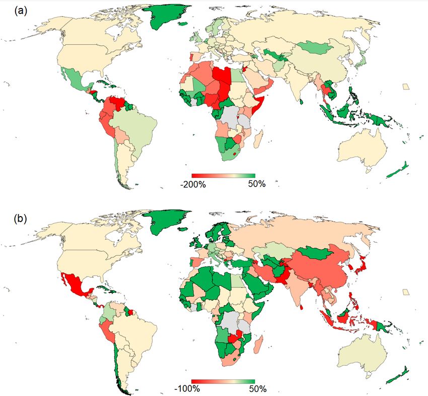
2028                                                                                  S. Tamea et al.: 1961–2016 CWASI database

Table 1. Data sources used to prepare the CWASI database.

   Variable                               Years      URL                                     Reference                  Access date
   Crop production, yield, and            1961–      http://www.fao.org/faostat/en/          FAOSTAT (2019a)            Oct 2019
   harvested areas                        2016       #data/QC
   Production of processed crops          1961–      http://www.fao.org/faostat/en/          FAOSTAT (2020a)            Jan 2020
                                          2016       #data/QD
   Detailed trade matrices                1986–      http://www.fao.org/faostat/en/          FAOSTAT (2019b)            Oct 2019
                                          2016       #data/TM
   Animal-based primary production        2000       http://www.fao.org/faostat/en/          FAOSTAT (2020b)            Mar 2020
                                                     #data/QL
   Animal-based processed                 2000       http://www.fao.org/faostat/en/          FAOSTAT (2020c)            Mar 2020
   production                                        #data/QP
   Live animals                           2000       http://www.fao.org/faostat/en/          FAOSTAT (2020d)            Mar 2020
                                                     #data/QA
   Reference uWF of crop-based            2000      https://waterfootprint.org/              Mekonnen and Hoekstra      Mar 2020
   products                               (average) en/resources/waterstat/                  (2010a)
                                                    product-water-footprint-statistics/
   Reference uWF of animal-based          2000      https://waterfootprint.org/              Mekonnen and Hoekstra      Mar 2020
   products                               (average) en/resources/waterstat/                  (2010b)
                                                    product-water-footprint-statistics/

Figure 1. Commodities considered in the analysis, split into nine categories: number of commodities in the trade and production dataset.
Icons designed by Freepik from Flaticon (https://www.flaticon.com/, last access: 5 May 2021).

pairs, per commodity, and per year, for the commodities in-            tions of the exporting and the importing countries, which are
cluded in the CWASI dataset), and the number of records re-            usually different, with a mean (absolute) relative difference,
ported by each country is detailed in Fig. 2. These records            across all goods, countries, and years, of 61 %. The choice of
are used to reconstruct the trade matrix M for each com-               a value from two double records is called “reconciliation”,
modity and year, having dimensions 255 × 255 and showing               and the method adopted here is based on the identification of
the exporting countries in the rows and the importing coun-            the most reliable reporting country among the two involved
tries in the columns. The matrix element M(i, j ) thus iden-           in each flow, and the use of the flow being reported by it. The
tifies the trade flow from country i to country j , which is           reliability of countries is measured per commodity and per
clearly different than the flow from country j to country i,           year with a data-based approach detailed below and adapted
i.e., M (i, j ) 6 = M(j, i). Sub-national trade is not considered      from Gehlhar (1996).
in these matrices, and the terms on the diagonals are zeros.
    In the construction of trade matrices, one should consider         Country reliability
that the same trade flow can be reported twice in the FAO-
STAT database, once by the exporting country and once by               For each product, p, and year, t, two trade matrices are built,
the importing country. When a trade flow is reported by only           one matrix collecting all “Importer-Reported” flows and the
one of the two countries, the reported flow is used to con-            other matrix collecting the “Exporter-Reported” flows. The
struct the matrix (single record); this is the case for 40 % of        matrices have the same structure and dimensions, with the
records in the database. All other records are “double” (re-           exporter countries in the rows and the importing countries in
ported twice) and require a comparison between the declara-            the columns. Then a reliability index is calculated for each
                                                                       country, c, differentiating between import and export. First,

Earth Syst. Sci. Data, 13, 2025–2051, 2021                                                https://doi.org/10.5194/essd-13-2025-2021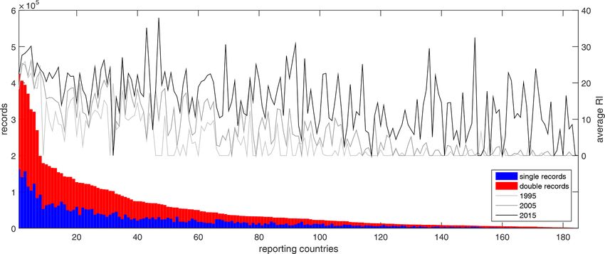
S. Tamea et al.: 1961–2016 CWASI database                                                                                     2029

an accuracy measure (A) is defined for every flux, from coun-       on average, by a larger reliability, while countries less in-
try i to country j , as                                             volved in trade have lower average reliability, which used to
                                                                    be very low in the past. Current RI values, instead, are more
               |IR (i, j ) − ER (i, j )|                            uniform across countries. Having computed all reliability in-
A (i, j ) =                                 ,                (1)
              max {IR (i, j ) , ER (i, j )}                         dexes, the “reconciled” trade matrix for each good and year
with IR (i, j ) being the importer-reported trade flux and          is built, combining importer-reported and exporter-reported
ER (i, j ) being the exporter-reported flux. The measure is         data. Each matrix element M(i, j ) is taken from the IR or
modified from Gehlhar (1996) to maintain the conceptual             ER matrix if the importing country j or the exporting i has
symmetry between import and export. The smaller the mea-            a larger reliability index. Where the reliability indexes are
sure, the more similar the information reported by the im-          equal, the country with larger acceptable fluxes is chosen.
porting and exporting country. Then, the reliability of each
country is measured, separately for import and export, based        3     Unit water footprint
on the comparison between the flows reported by the country
and by its trade partners. For every country, c, the reliabil-      The unit water footprint measures the amount of water re-
ity index for imports, RIimp (c), and for exports, RIexp (c), is    quired to produce a unit amount of product and it can be
defined as follows:                                                 expressed as m3 t−1 or, equivalently, as L kg−1 . The present
                   Pacc                                             work considers the sum of green water (originating from
                      j IR (j, c)                                   rainfall) and blue water (originating from surface water and
RIimp (c) = Pall                        ,                   (2)
                                                                    groundwater bodies). Depending on the type of commodity,
                j IR (j, c) − IR (w, c)
                   Pacc                                             different approaches are applied for the computation of the
                      i ER (c, i)                                   unit water footprint. In the present work we propose a dif-
RIexp (c) = Pall                          ,
                i ER (c, i) − ER (c, w)                             ferentiation between the uWF of production (uWFp) and the
                                                                    uWF of supply (uWFs). The uWFp refers to locally produced
where IR (j, c) is the flux from country j to c, as reported by
                                                                    crops whose water footprint depends on the actual crop evap-
c (importer-reported), and ER (c, i) is the flux from c to any
                                                                    otranspiration and crop yield, with annual estimates starting
country i, as reported by c (exporter-reported), respectively.
                                                                    in 1961. The uWFp is a suitable indicator to assess the WF of
6 all is the sum of all import or export fluxes reported by c,
                                                                    agricultural production. The uWF, instead, refers to the do-
and 6 acc is the sum of acceptable fluxes only, defined as the
                                                                    mestic supply, which relies both on local production and on
fluxes whose accuracy A (Eq. 1) is smaller than an accep-
                                                                    international trade. Country-scale domestic supply is avail-
tance threshold, set to 20 % as in Gehlhar (1996). IR (w, c)
                                                                    able for human consumption, food manufacturing, feed for
and ER (c, w) in Eq. (2) are, respectively, the import from
                                                                    livestock, and export towards other countries. The impossi-
and the export to the worse partner w defined as the ones
                                                                    bility to track local production and imports into consumption
having the maximum (worse) flow-weighted accuracy mea-
                                                                    and exports, within each country, makes the uWFs the best
sure (WA) defined, for import and export fluxes, as
                                                                    indicator to be used in conjunction with consumption and ex-
                          IR (j, c)                                 port data. The uWF is computed averaging local production
WAcimp (j ) = A (j, c) · Pall         ,                      (3)    and imports, after having identified the countries of origin of
                          j IR (j, c)                               the goods with an appropriate procedure applicable from the
                         ER (c, i)                                  year 1986.
WAcexp (i) = A (c, i) · Pall         .
                         i ER (c, i)
                                                                       For primary crops, it has been possible to estimate both
                                                                    the uWFp and the uWFs. Processed crops are produced from
A (j, c) is the accuracy level of flux IR (j, c), and A (c, i) is   a root product which may or may not originate from local
the accuracy level of flux ER (c, i); the denominators are, re-     production. The absence of systematic FAO data about the
spectively, the sum of all imports and all exports reported by      production of processed crops prevents the differentiation
country c.                                                          between the unit water footprint of production and of sup-
   Reliability indexes are calculated by country, commodity,        ply. Therefore, processed crops considered in this study will
year, and flow direction (import and export). This is because       have a single unit water footprint, depending on country and
the reliability of a country in reporting import and export         year, computed from the uWFs of the root product. Finally,
may be different; the attitude of a country to over-report or       animal-based products are considered here only with the Wa-
under-report may differ by products, e.g., depending on tax-        terStat values, without temporal variability.
ation; and the reliability of a country may change in time,
e.g., according to socio-political factors. The direction- and
                                                                    3.1    Unit water footprint of locally produced primary
commodity-averaged RI of reporting countries are shown in
                                                                           crops in time
Fig. 2 with the darker (lighter) line corresponding to the
newest (oldest) values. Countries more involved in trade and        When considering the production of primary crops, the unit
reporting more information (to the left) are characterized,         water footprint of production, uWFp, is a function of the ac-

https://doi.org/10.5194/essd-13-2025-2021                                           Earth Syst. Sci. Data, 13, 2025–2051, 2021
2030 S. Tamea et al.: 1961–2016 CWASI database
Figure 2. Number of single and double records per reporting country (including all partners, all goods, and all years). The right axis indicates
the country-specific reliability index averaged over all goods in three separate years.
tual evapotranspiration along the growing period of the crop other hand, the uWF is less sensitive to hydro-climatic con-
and the actual crop yield. Due to precipitation, evapotranspi- ditions than actual evapotranspiration because it is defined
ration, and yield fluctuations, the uWFp exhibits significant as the ratio between evapotranspiration and yield, both react-
spatiotemporal variability. We computed the uWFp in a given ing with equal signs to hydro-climatic fluctuations (see, e.g.,
year by means of the fast-track (FT) method, introduced and Doorenbos et al., 1979). Additional indications about the un-
substantiated in Tuninetti et al. (2017). This method is based certainty associated with the fast-track method are provided
on the use of the WaterStat database (Mekonnen and Hoek- in Sect. 5.1.
stra, 2010a, 2010b) for expressing the spatial variations in
evapotranspiration and on a ratio of agricultural yields for ex-
3.2 Primary-equivalent trade matrix
pressing the temporal variability of the unit water footprint,
not detailed in WaterStat. For the correct identification of countries of origin of the
According to the fast-track method, the unit water foot- crops traded internationally, the reconstruction of a primary-
print of an agricultural product p produced in country c in equivalent trade matrix, Meq , is necessary (Kastner et al.,
year t, i.e., uWFpc,p,t , reads 2011). This is defined as
Yc,p,T X fv
uWFpc,p,t = uWFpc,p,T · , (4) Meq = Mp + Mdp · , (5)
Yc,p,t dp
fp
where uWFpc,p,T is the reference unit water footprint pro- where Mp is the trade matrix of any root product, Mdp is the
vided by WaterStat (Mekonnen and Hoekstra, 2010a, b) trade matrix of the derived products (dp), and fp and fv are
corresponding to an average in the period T = 1996–2005, the product fraction and value fraction which convert the de-
Yc,p,T is the average crop yield over the same period T , and rived products into a root-product equivalent quantity. The
Yc,p,t is the annual crop yield in a generic year t in the range summation is extended to all derived products which origi-
1961–2016. The average crop yield is obtained as an aver- nate from the same root product and, in the case of a multi-
age of the annual yields in the years 1996–2005, weighted step supply chain, Eq. (5) is applied iteratively until reach-
by the harvested areas across the years in country c, based on ing a root product that is also a primary crop. The product
FAOSTAT data (FAO, 2019a). fraction, fp , is defined as the weight of a derived product
The fast-track method keeps the actual evapotranspiration obtained from a weight unit of input product. For example,
of crops implicitly constant, equal to the long-term average a weight unit of nuts with shells leads to fp (< 1) tons of
used in the WaterStat statistics, but this hypothesis should shelled nuts. The value fraction, fv , is the market value of
come at no surprise. On the one hand, yield implicitly ex- the derived product divided by the aggregated market value
presses many factors, including climatic conditions, water of all derived products resulting from a ton of input product.
availability, soil fertility, and agricultural practices among For example, in a production process of wheat flour there are
others, and temporal yield variations dominate the variability other economically valuable by-products (e.g., wheat germs
of the water volumes used (evapotranspired) by crops. On the to feed animals); hence, the value of wheat flour constitutes
Earth Syst. Sci. Data, 13, 2025–2051, 2021 https://doi.org/10.5194/essd-13-2025-2021S. Tamea et al.: 1961–2016 CWASI database 2031
only a portion (i.e., the value fraction) of the total value gen- where the R matrix identifies where the supply of each coun-
erated by the process. Product fractions and value fractions try originates from and I is the identity matrix. For further
used in the CWASI database are time- and space-invariant details and exemplification, see Kastner et al. (2011).
and are taken from Mekonnen and Hoekstra (2010a, b), as By knowing the uWFp of the primary crop in such coun-
well as the root products and the full supply chains of the tries, we can now define the unit water footprint of supply in
considered commodities. country c and year t of the primary product p, i.e., uWFsc,p,t ,
as
3.3 Supply-side unit water footprint of primary crops 255
X Rp,t (j, c)
uWFsc,p,t = uWFpj,p,t · . (9)
The country supply of a primary crop results from the sum of S c,p,t
j =1
local production and imports, where imports may occur from
producing or non-producing countries, the latter case testi- The evaluation of uWFs corresponds to a weighted average
fying a re-export of goods produced elsewhere. Therefore, of the uWFp values, where the weights are the actual frac-
the unit water footprint of supply, uWFs, is proportionally tions of supply, S, traced back to their origins. Equation (9)
contributed by local production and by trade, specifying the is valid for every primary crop p and year t, considering that
relative contribution of every country from which the goods trade matrices, production vectors, and uWFp values change
originated from, considering re-exports and the processing from year to year. It is worth noticing that because the trade
of goods, if necessary. For each primary-equivalent crop and matrices are available from 1986 only, the uWFs can be built
each year, we can define a column vector, S, containing the from that year only.
supply of all countries as rows. This vector is calculated as
the sum of the production vector, P , and of the imports ob- 3.4 Unit water footprint of processed crops in time
tained from the bilateral trade matrix Meq , where Meq (i, j )
identifies the trade flow from i to j as Processed crops are based on the processing of root products,
which are available as a country’s supply. The time-varying
S = P + M0eq · I , (6) unit water footprint thus depends on that of the root product
and on the conversion factors (i.e., Hoekstra et al., 2011),
where I is a column vector of ones (i.e., a summation vector)
and M0eq is the trade matrix transposed. Hence, the uWFs of fv
uWFc,dp,t = uWFsc,p,t · , (10)
a country depend both on the domestic uWFp (through P ) fp
and on the uWFp of the origin countries, where the product
is produced. where uWFc,dp,t is the unit water footprint of the processed
In order to trace the actual origin of the country’s sup- crop (or derived product, dp); uWFsc,p,t is the unit water
ply, namely tracing its origin back to the country where it footprint of supply of the root product from which it derives
was produced, we adopt the approach proposed by Kastner (p); c and t are country and year, respectively; fp is the prod-
et al. (2011). First, we define a matrix R, where each ele- uct fraction; and fv is the value fraction of the processed crop
ment R(i, j ) is the quantity of supply in country i that is pro- (see Sect. 3.2). The method takes into account the temporal
duced in country j . A first approximation of R can be based variability associated with both the crop production, through
on reported flows only and is equal to the sum of a diagonal the fast-track method applied to the primary crop, and the
matrix with elements of the P vector on the diagonal, i.e., evolution of trade, through the Kastner’s method applied to
diag (P ), and the transposed trade matrix, M0eq . However, this the crop supply; the method does not include water inputs
approximation misses the fact that exporting countries may for processing of goods. When supply chains are formed by
obtain the exported products not only from local production, multiple steps, for example in the case of bread, made with
but also from import. To account for this fact, a matrix of flour, made in turn with wheat, Eq. (10) is applied routinely
export shares, X, can be defined as at each step. Within the CWASI dataset, the longest supply
chain is made of four steps, leading to final products such as
X = M0eq · diag S −1 , (7) refined sugar or chocolate.
Equation (10) describes the unit water footprint without
where X(i, j ) is the share of country j ’s supply that is ex- differentiating between production and supply. This is be-
ported to country i. The term diag S −1 denotes a diagonal cause the absence of FAOSTAT data of production of most
matrix made up by the reciprocal elements of S. In turn, the processed crops (FAO, 2020a) hinders the application of the
imported and re-exported products may partly originate from Kastner’s method (Sect. 3.3) and thus an explicit accounting
local production and import, and so on, recursively. It has of countries of origin of trade, as in the case of primary crops.
been shown by Miller and Blair (2009) that such a procedure However, the trade of processed crops is implicitly taken into
converges to account in the procedure, thanks to the use of the primary-
equivalent trade matrix (Eq. 5), which serves to compute the
R = (I − X)−1 · diag(P ), (8) uWFs of the primary crop. For the very few derived products
https://doi.org/10.5194/essd-13-2025-2021 Earth Syst. Sci. Data, 13, 2025–2051, 20212032 S. Tamea et al.: 1961–2016 CWASI database
without indication of the root product (Mekonnen and Hoek- WaterStat database (e.g., USSR), the reference value of uWF
stra, 2010a), an association is made which is based on logical required in Eq. (4) is computed as a production-weighted av-
considerations (such as “Figs dried” deriving from “Figs”) or erage of the values of countries belonging to the union and
on similitudes of products. The “Sugar” products (raw sugar, available in WaterStat. This average value is then used to re-
refined sugar, etc.) were also missing the root product, likely construct the annual uWF from 1961 up to the year of the
due to a lack of information. For these products, we have disaggregation. After converting the agricultural production
traced back the root product to the product most largely avail- into water volumes, the overall water footprint of produc-
able as country supply (either “Sugar beet” or “Sugar cane”). tion is obtained by summing across all commodities. Care
must be used to avoid double accounting of water footprints
3.5 Unit water footprint of animal-based commodities
of primary and derived goods. For this reason, only primary
products must be considered in aggregated production data.
Animal-based commodities considered in FAOSTAT belong In particular, when dealing with animal-based commodities,
to three groups: “Live animals”, “Livestock primary”, and one should avoid the inclusion of both livestock and the cor-
“Livestock processed” (FAO, 2020b, c, d). Products of the responding products as well as the crops used to feed the live-
first group are given in heads, which have been converted stock. Primary, or single-accounting, products to be included
to tons according to FAO conversion factors (FAO, 2013). in the sum are indicated in the Appendix, in Table A1.
The missing conversion values for some countries have been Computation of the supply-side unit water footprint of
assigned with an average value of the same or similar ani- goods enables the fast computation of the water footprint as-
mals. Products of the second group are here considered to sociated with the consumption of commodities, under the hy-
be primary products, while live animals are only included in pothesis that consumption (and export) shares the same mix
trade data. Due to the lack of reliable data about country- of local and imported goods with the country’s supply. The
specific animal diets and their temporal variability as well as water footprint of consumption in a country and year can thus
the lack of detailed trade matrices of feed crops, we do not be obtained by multiplying the consumed quantity of each
currently provide a time-dependent unit water footprint for good by the unit water footprint of supply, uWFs (per com-
the animal-based commodities. Similarly, we do not provide modity, country, and year), and then summing across all com-
a supply-side uWF. Nevertheless, we include these products modities. In this case, there are no double-accounting issues.
in the present database adopting the country-specific values For commodities occasionally missing their uWF values, the
of unit water footprint provided by WaterStat (Mekonnen last available value or the uWFp can be used instead.
and Hoekstra, 2010b). These values take into account the The virtual water trade is obtained by multiplying trade
feed–animal–commodity global supply chain, considering data (FAO, 2019b), expressed in metric tons, by the unit wa-
locally produced and imported feed (Mekonnen and Hoek- ter footprint of supply, uWFsc,p,t , of the exporting country.
stra, 2012), but are only available as time-averaged values Thanks to the new definition of supply-side unit water foot-
over the period 1996–2005. Here data are generically refer- print, this computation allows one to take into account the
enced to the year 2000 and are arranged consistently with the origin of goods, which are traced back to their origin coun-
rest of the CWASI database. tries along the supply chain. In the few cases of goods ex-
ported from countries not having an associated uWF (less
than 1 % of all existing links, mainly from minor countries
4 Virtual water trade and water footprint indicators
or remote islands), the global average uWF of supply is used,
4.1 Water footprint and VWT data
weighted by all countries’ exports. Virtual water trade asso-
ciated with animal-based commodities is given for the year
The water footprint of agricultural production in a coun- 2000 only, consistently with their unit water footprint, with
try and year is obtained by multiplying the production data the uWFp used for the conversion, since a uWF is not avail-
(FAO, 2019a, 2020a, b, c, d), expressed in metric tons, by the able for these commodities yet.
corresponding (commodity, country, year) unit water foot-
print, considering the unit water footprint of production, 4.2 The uWF index
uWFpc,p,t , in the case of primary crops. A problem arises
when a country was not a producer in the 1996–2005 decade; In the Results section, the (volumetric) water footprint and
thus it does not have an associated value in the WaterStat the virtual water trade are summed across different com-
database. In such a case, the uWF in the closest produc- modities, and the overall trends are assessed in time. How-
ing country within a 10◦ distance is taken; if no produc- ever, the unit water footprint of different commodities cannot
ing countries are found (e.g., in the case of remote islands be summed across commodities but only for one commod-
or small producing areas), then the global average weighted ity at a time. To overcome such a problem, an appropriate
by production is used. In the case of countries having ex- index is constructed analogously to economic indices aggre-
perienced political discontinuity, for example belonging to a gating prices of different commodities, such as the agricul-
larger country before the years 1996–2005 considered in the ture producer price index (in FAOSTAT) calculated with the
Earth Syst. Sci. Data, 13, 2025–2051, 2021 https://doi.org/10.5194/essd-13-2025-2021S. Tamea et al.: 1961–2016 CWASI database 2033
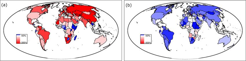
database), the uWFp values at the beginning and at the end
of the considered period are very different. Figure 4 shows
the relative change of the uWFp of wheat in 1961 and 2016
with respect to the 1996–2005 average. The variation is quite
uniform worldwide with improvements (decreases in uWF)
in both periods which are consistent with the period lengths.
Extreme variations have occurred in China (largest improve-
ment from 1961) and in African countries, showing large im-
provements in time, but also occasional worsening due to un-
stable socio-economic conditions. It should be noticed that a
few countries worldwide do not produce wheat or miss FAO-
STAT or WaterStat data: in such cases, countries are left in
white.
A comparison between the uWF of production and sup-
ply of primary crops is very informative. Figure 5 highlights
the absolute difference for wheat and soybean with red in-
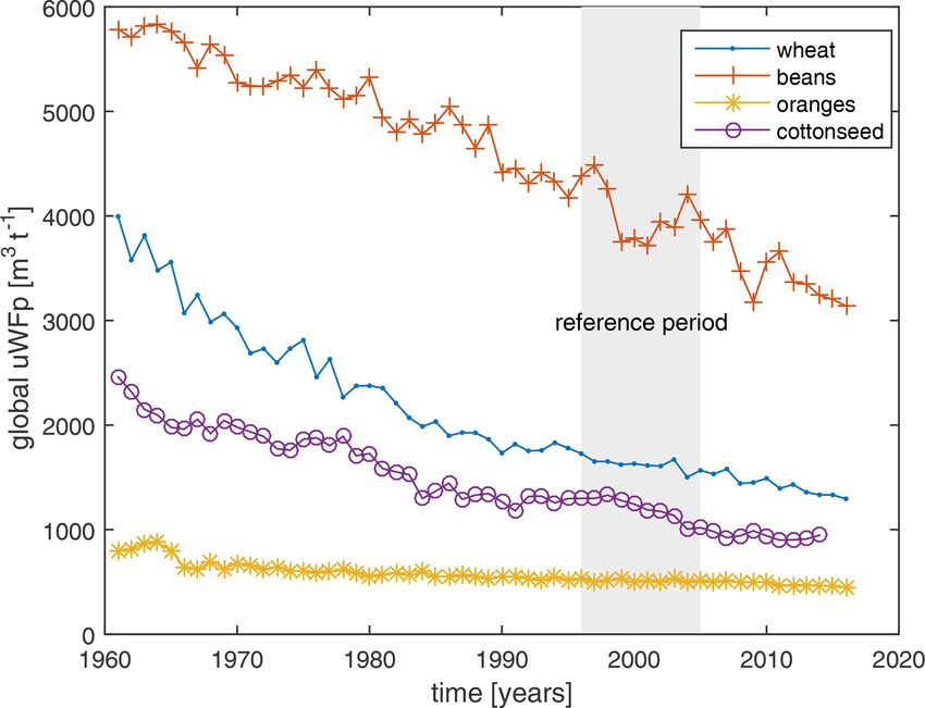
Figure 3. Production-weighted global uWFp along the period dicating countries where the uWFs is smaller than uWFp
1961–2016 for wheat, beans, oranges, and cotton. and green for the opposite. The more intense the red color,
the more efficient the crop import in saving global water re-
sources because the imported crops are produced with lower
Laspeyres approach. The index is built as the inverse ratio uWF than the local uWF of production. This is the case for
between the WF of production (m3 ) of all commodities (i) in several African countries, some South American ones, and
all countries (c) in the year 2000 and the WF obtained with Thailand for wheat and several South Asian countries for
the same quantities (year 2000) but with uWF in year t, i.e., soybeans. Conversely, the more intense the green, the more
P efficient the global production, compared to imports. The
i,c uWF (i, c, t) · P (i, c, 2000) extreme case of non-producing (but importing) countries is
I (t) = P · 100. (11)
i,c uWF (i, c, 2000) · P (i, c, 2000) highlighted by bold contours. This is observed in several Far
East countries for wheat and by most African countries for
In such a way, I (t) expresses the variation in uWF across all soybeans.
agricultural commodities, weighted by the productions in the Considering all commodities together, the analysis of tem-
year 2000, P (i, c, 2000). A similar index as in Eq. (11) can poral evolution requires the use of a uWF index, which is
also be built referring to categories of goods by aggregating applied to the uWF of production and uses the agricultural
only the commodities belonging to one single category. production of the year 2000 as weight (Eq. 11). The index is
shown in Fig. 6 (left) and decreases monotonically in time,
5 Results being at +60 % in 1961 and −10 % in 2016. The trend is
less marked than in Fig. 3 because all commodities, and
The importance of considering a time-dependent unit water not only wheat, are being considered in the index, including
footprint is highlighted in Fig. 3, which shows the tempo- those not having a uWF varying in time (e.g., animal-based
ral trends of the global average uWF of production of some products, as made explicit in Fig. 6, right). If one should in-
commodities (other major crops are shown in Tuninetti et clude the temporal evolution of animal-based commodities,
al., 2017). The global average is computed by weighting the the temporal variation in the index would be more marked.
uWFp of each country by the country production of the crop. The uWF index built by category of commodities, shown in
The relevance of the temporal change is evident for example Fig. 6 (right), allows one to find similarities and differences.
for wheat, with values ranging from 4000 to 1200 m3 t−1 in In time, the uWF of production of cereals has improved con-
the considered period. The values considered in WaterStat re- stantly up to the 1990s. Then, after a period of stagnation, it
fer to the period T = 1996–2005, highlighted by a grey shade has improved constantly again in the last 15 years. A simi-
in Fig. 3: it is clear that the average value in such a reference lar dynamic, even if less regular, is observed in the seeds/oil
period is scarcely representative of the whole period consid- category. Fruits and vegetables show a lower range of vari-
ered in the present dataset. It is thus very important to con- ability without stagnation in the period 1990–2000. Luxury
sider the temporal variability of unit water footprint, espe- foods show the only increasing dynamic observed in the last
cially in analyses spanning long periods or periods different decade, dictated by coffee and cocoa beans, while non-edible
than the years 1996–2005. goods show a more recent improvement, with the decrease
The temporal variation in the uWF of production of crops in uWFp starting only in the mid-1970s and concluding the
is marked all over the world. If compared to the values period with a small increase, mostly associated with natural
averaged over the period 1996–2005 (as in the WaterStat rubber.
https://doi.org/10.5194/essd-13-2025-2021 Earth Syst. Sci. Data, 13, 2025–2051, 20212034 S. Tamea et al.: 1961–2016 CWASI database Figure 4. Relative change in the uWFp of wheat in 1961 (a) and 2016 (b) with respect to the average in 1996–2005, using identical color ranges: red (blue) colors identify higher (lower) values and color intensity scales with change values. (Maps are created with MATLAB®R14 software, Mapping Toolbox v.2.0.3.) Figure 5. Percentage difference between the uWF of production and supply of wheat (a) and soybean (b) in the year 2016, calculated as the difference between uWFs and uWFp, normalized by uWFs. Bold green countries do not produce the crop; hence they only have a supply-side uWF. (Maps are created with Microsoft Power Map for Excel, ©Microsoft.) The time-varying uWF in the CWASI database is used to almost 2400 km3 yr−1 in the considered period. Major cate- assess the temporal evolution of virtual water trade across the gories are cereals, luxury food, and seeds/oils, followed by years, considering the contribution of different categories of vegetables and meat. All categories show an increase in as- goods. Figure 7 updates previous versions published in the sociated VWT, with non-edible goods showing the minimum literature (e.g., Konar el at., 2011; Carr el at., 2013; Tuninetti increase (32 %) and seeds/oils showing the largest increase et al., 2017) by introducing the temporal variability of the (more than 3-fold). The relative contribution of each category uWF of crop-based goods and expanding the number of con- has changed in time, with the most relevant change shown sidered crops. Total VWT has increased from about 900 to by cereals, having decreased their contribution from 32 % to Earth Syst. Sci. Data, 13, 2025–2051, 2021 https://doi.org/10.5194/essd-13-2025-2021
S. Tamea et al.: 1961–2016 CWASI database                                                                                               2035

Figure 6. Temporal variability of uWF indexes weighted with agricultural production (solid) and export (with dots) in the year 2000,
aggregated across all goods (left) and (right) split into the nine categories of goods.

                                                                            with the fast-track method is also lower or comparable to the
                                                                            model uncertainty associated with the water footprint assess-
                                                                            ment, verified by a comparison with the WaterStat values (see
                                                                            Tuninetti et al., 2017).
                                                                               The fast-track method, initially applied to four crops
                                                                            (wheat, maize, rice, and soybeans), has been extended in the
                                                                            CWASI database to a large set of primary products, includ-
                                                                            ing cereals, fruits, vegetables, seeds, luxury food, and non-
                                                                            edibles. The extension is justified by the fact that similar error
                                                                            ranges are expected in all crops, because water stress affects
                                                                            the evapotranspiration of different crops in a similar way, the
                                                                            only difference being the phases of the growing periods af-
                                                                            fected by water stress and the crop coefficients describing the
                                                                            plant water requirements. Water stress is assumed not to af-
                                                                            fect irrigated crops, implying that actual evapotranspiration
                                                                            matches the crop maximum evapotranspiration in irrigated
Figure 7. Global virtual water trade (as derived from export data)          conditions. Uncertainty associated with the fast-track method
from 1961 to 2016 considering the nine categories of goods from             has been sparsely checked on other crops than the first four,
Fig. 2.                                                                     and the range of errors found in Tuninetti et al. (2017) has
                                                                            been confirmed. Considering the hypothesis of a long-term
                                                                            average actual evapotranspiration of crops, we suggest using
21 % of total virtual water trade. The growth of animal-based               single-year data of uWF with care, as well as WF and VWT.
products is remarkable, but it should be specified that it only             It is precautionary to consider single-year data in a temporal
reflects the increased trade quantity without considering the               perspective, such as a trend analysis, or use a multi-year av-
temporal variability of uWF.                                                erage to minimize the error and avoid misinterpretations of
                                                                            year-specific results.
5.1   Uncertainties and limitations                                            A minor point of caution is related to the supply-side uWF,
                                                                            which averages a country’s local production and import. This
Despite the large amount of information and the many im-                    variable is the best estimate to be used in association with
provements provided with the CWASI database, the data                       countries’ export and consumption, unless more detailed in-
uncertainty and a few cautions are worth being mentioned.                   formation is available about the origin of the country’s export
The time-varying unit water footprints of crops and crop-                   or consumption. If local production or import should prevail,
based commodities are estimated with a simplified method                    compared to the average country’s supply, a more precise
(the fast-track method) that has been thoroughly assessed                   weighted average of unit water footprint will be enabled by
before applying it widely. For example, the fast-track esti-                such information.
mates of unit water footprint were compared to the results                     Concerning the uWF of animal-based commodities, as
of a complete model based on a daily soil water balance fed                 well as their WF and the VWT, they are here reported for the
by year-specific hydro-climatic variables, and the errors were              year 2000 only, referring to the average over the years 1996–
found to be within a 10 % range (Tuninetti et al., 2017). The               2005 in the WaterStat database. Where necessary, these val-
uncertainty introduced in the unit water footprint estimates

https://doi.org/10.5194/essd-13-2025-2021                                                   Earth Syst. Sci. Data, 13, 2025–2051, 2021
2036 S. Tamea et al.: 1961–2016 CWASI database ues have been applied to production and trade occurring in different years (see Figs. 6 and 7), although caution with such applications should be exercised. This limitation can be over- come when reliable data on the country-specific feed com- position and diet of animals will become available along the considered time period. 6 Data availability Data are available on the Zenodo repository at https://doi.org/10.5281/zenodo.4606794 (Tamea et al., 2020). 7 Conclusions The globalization of water resources through the interna- tional trade of food and agricultural goods is a remarkable global environmental change of our times, and the scientific community is devoting great effort to study it. The quantifi- cation of the volumes of water involved in the production and trade of agricultural goods is a key tool to investigate the water–food–trade nexus issues. This study presents an open- source database specifically developed for this purpose. The main outcome of this study is the time-varying unit water footprint for the years 1961–2016 and the virtual water trade matrices for the years 1986–2016 of hundreds of commodi- ties from the food and agricultural sector. The water foot- print of production per commodity is also available annually in the period 1961–2016. The current database includes a to- tal of almost 30 million data, half of them being elements of the trade matrices. The introduction of a supply-side es- timate of the unit water footprint brings much more detail in the water footprint accounting. This is a new concept and a key tool in the expedited and accurate accounting of the virtual water trade and of the water footprint of consump- tion. The supply-side unit water footprint overcomes previ- ous problems related to the non-consideration of re-export, and it also enables a more accurate assessment of virtual wa- ter trade, with the correct identification of countries of origin of traded goods. The open-source database presented in this work aims to help the scientific community and policy makers to quan- tify and investigate the complex linkages between the global food system and water resource issues. Potential applica- tions of the CWASI dataset range from supporting national- scale policies of water management as well as agricultural policies oriented to the optimization of water use or, ul- timately, to provide indications for price formation or for trade agreements based on the efficient and sustainable use of water resources worldwide. The CWASI database is shared through the Zenodo online open-access repository (Tamea et al., 2020), and it is planned to be improved upon and updated in the future, capitalizing contributions from the overall sci- entific community. Earth Syst. Sci. Data, 13, 2025–2051, 2021 https://doi.org/10.5194/essd-13-2025-2021
S. Tamea et al.: 1961–2016 CWASI database                                                               2037

Appendix A: Commodities and countries in the
CWASI database

Commodities included in the CWASI database are listed in
Table A1, which shows the commodity name, the FAO code,
the presence of data in different database variables (1: yes, 0:
no, 1∗ : without temporal variability), the presence of trade
data (1: yes, 0: no), the indication of primary items and
the associated category. Countries considered in the CWASI
database are listed in Table A2, which include the coun-
try name, the FAO code, the position in the CWASI vec-
tors/matrices, the indication of reporting (1) or non-reporting
(0) countries, and the presence of discontinuities in the con-
sidered period.

https://doi.org/10.5194/essd-13-2025-2021                          Earth Syst. Sci. Data, 13, 2025–2051, 2021
2038                                                                           S. Tamea et al.: 1961–2016 CWASI database

Table A1. List of commodities in the CWASI database.

        Commodity name                        FAO code   In uWFp   In uWFs   In VWT   In WFP   Primary   Category
        Wheat                                       15         1        1         1        1        1    Cereals
        Flour of wheat                              16         0        1         1        0        0    Cereals
        Macaroni                                    18         0        1         1        0        0    Cereals
        Bread                                       20         0        1         1        0        0    Cereals
        Bulgur                                      21         0        1         1        0        0    Cereals
        Rice, paddy                                 27         1        1         0        1        1    Cereals
        Rice husked                                 28         0        1         0        0        0    Cereals
        Rice, milled/husked                         29         0        1         0        0        0    Cereals
        Rice – total (rice milled equival.)         30         0        0         1        0        0    Cereals
        Rice milled                                 31         0        1         0        0        0    Cereals
        Rice broken                                 32         0        1         0        0        0    Cereals
        Rice flour                                  38         0        1         0        0        0    Cereals
        Beverages, fermented rice                   39         0        1         1        0        0    Lux-foods
        Barley                                      44         1        1         1        1        1    Cereals
        Barley pearled                              46         0        1         1        0        0    Cereals
        Barley flour and grits                      48         0        1         0        0        0    Cereals
        Malt                                        49         0        1         1        0        0    Cereals
        Beer of barley                              51         0        1         1        0        0    Lux-foods
        Maize                                       56         1        1         1        1        1    Cereals
        Germ, maize                                 57         0        1         1        0        0    Cereals
        Flour of maize                              58         0        1         1        0        0    Cereals
        Maize oil                                   60         0        1         1        0        0    Seeds and oils
        Rye                                         71         1        1         1        1        1    Cereals
        Flour of rye                                72         0        1         0        0        0    Cereals
        Oats                                        75         1        1         1        1        1    Cereals
        Oats rolled                                 76         0        1         1        0        0    Cereals
        Millet                                      79         1        1         1        1        1    Cereals
        Sorghum                                     83         1        1         1        1        1    Cereals
        Buckwheat                                   89         1        1         1        1        1    Cereals
        Quinoa                                      92         1        1         0        1        1    Cereals
        Fonio                                       94         1        1         1        1        1    Cereals
        Triticale                                   97         1        1         1        1        1    Cereals
        Canary seed                                101         1        1         1        1        1    Non-edible
        Mixed grain                                103         1        1         1        1        1    Cereals
        Flour, mixed grain                         104         0        1         1        0        0    Cereals
        Cereals, nes                               108         1        1         0        1        1    Cereals
        Flour, cereals                             111         0        1         1        0        0    Cereals
        Cereal preparations, nes                   113         0        1         1        0        0    Cereals
        Potatoes                                   116         1        1         1        1        1    Vegetables
        Potatoes flour                             117         0        1         1        0        0    Vegetables
        Frozen potatoes                            118         0        1         1        0        0    Vegetables
        Tapioca of potatoes                        121         0        1         0        0        0    Vegetables
        Sweet potatoes                             122         1        1         1        1        1    Vegetables
        Cassava                                    125         1        1         1        1        1    Vegetables
        Flour of cassava                           126         0        1         0        0        0    Vegetables
        Tapioca of cassava                         127         0        1         0        0        0    Vegetables
        Cassava dried                              128         0        1         1        0        0    Vegetables
        Cassava starch                             129         0        1         1        0        0    Vegetables
        Yautia (cocoyam)                           135         1        1         0        1        1    Vegetables
        Taro (cocoyam)                             136         1        1         0        1        1    Vegetables
        Yams                                       137         1        1         0        1        1    Vegetables
        Roots and tubers, nes                      149         1        1         1        1        1    Vegetables

Earth Syst. Sci. Data, 13, 2025–2051, 2021                                        https://doi.org/10.5194/essd-13-2025-2021
You can also read