A DEEP VARIATIONAL APPROACH TO CLUSTERING SURVIVAL DATA
←
→
Page content transcription
If your browser does not render page correctly, please read the page content below

Published as a conference paper at ICLR 2022

A D EEP VARIATIONAL A PPROACH                                            TO     C LUSTERING
S URVIVAL DATA
 Laura Manduchi†,1 Ričards Marcinkevičs†,1 Michela C. Massi,2,3 Thomas Weikert,4
 Alexander Sauter,4 Verena Gotta,5 Timothy Müller,6 Flavio Vasella,6 Marian C. Neidert,7
 Marc Pfister,5 Bram Stieltjes4 & Julia E. Vogt1
 1
   ETH Zürich; 2 Politecnico di Milano; 3 CADS, Human Technopole; 4 University Hospital Basel;
 5
   University Children’s Hospital Basel; 6 University of Zürich; 7 St. Gallen Cantonal Hospital

                                              A BSTRACT
            In this work, we study the problem of clustering survival data — a challenging and
            so far under-explored task. We introduce a novel semi-supervised probabilistic ap-
            proach to cluster survival data by leveraging recent advances in stochastic gradient
            variational inference. In contrast to previous work, our proposed method employs
            a deep generative model to uncover the underlying distribution of both the ex-
            planatory variables and censored survival times. We compare our model to the
            related work on clustering and mixture models for survival data in comprehensive
            experiments on a wide range of synthetic, semi-synthetic, and real-world datasets,
            including medical imaging data. Our method performs better at identifying clus-
            ters and is competitive at predicting survival times. Relying on novel generative
            assumptions, the proposed model offers a holistic perspective on clustering sur-
            vival data and holds a promise of discovering subpopulations whose survival is
            regulated by different generative mechanisms.

1       I NTRODUCTION
Survival analysis (Rodrı́guez, 2007; D. G. Altman, 2020) has
been extensively used in a variety of medical applications to
infer a relationship between explanatory variables and a po-
tentially censored survival outcome. The latter indicates the
time to a certain event, such as death or cancer recurrence,
and is censored when its value is only partially known, e.g.
due to withdrawal from the study (see Appendix A). Classical
approaches include the Cox proportional hazards (PH; Cox
(1972)) and accelerated failure time (AFT) models (Buck-
ley & James, 1979). Recently, many machine learning tech-
niques have been proposed to learn nonlinear relationships
from unstructured data (Faraggi & Simon, 1995; Ranganath               Figure 1: Survival clustering.
et al., 2016; Katzman et al., 2018; Kvamme et al., 2019).
Clustering, on the other hand, serves as a valuable tool in data-driven discovery and subtyping of
diseases. Yet a fully unsupervised clustering algorithm does not use, by definition, the survival
outcomes to identify clusters. Therefore, there is no guarantee that the discovered subgroups are
correlated with patient survival (Bair & Tibshirani, 2004). For this reason, we focus on a semi-
supervised learning approach to cluster survival data that jointly considers explanatory variables
and censored outcome as indicators for a patient’s state. This problem is particularly relevant for
precision medicine (Collins & Varmus, 2015). The identification of such patient subpopulations
could, for example, facilitate a better understanding of a disease and a more personalised disease
management (Fenstermacher et al., 2011). Figure 1 schematically depicts this clustering problem:
here, the overall patient population consists of three groups characterised by different associations
between the covariates and survival, resulting in disparate clinical conditions. The survival distribu-
tions do not need to differ between clusters: compare groups 1 () and 3 ().
    †
        Equal contribution. Correspondence to {laura.manduchi,ricardsm}@inf.ethz.ch

                                                     1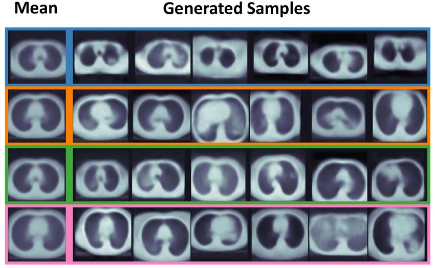
Published as a conference paper at ICLR 2022

Table 1: Comparison of the proposed model to the related approaches: semi-supervised clustering
(SSC), profile regression (PR) for survival data, survival cluster analysis (SCA), and deep survival
machines (DSM). Here, t denotes survival time, x denotes explanatory variables, z corresponds to
latent representations, K stands for the number of clusters, and L(·, ·) is the likelihood function.

                                            SSC     PR    SCA     DSM     VaDeSC
                     Predicts t?             7      3      3       3        3
                     Learns z?               7       7     3       3        3
                     Maximises L (x, t)?     7      3      7       7        3
                     Scalable?               7       7     3       3        3
                     Does not require K?     7      3      3       7         7

Clustering of survival data, however, remains an under-explored problem. Only few methods have
been proposed in this context and they either have limited scalability in high-dimensional, unstruc-
tured data (Liverani et al., 2020), or they focus on the discovery of purely outcome-driven clusters
(Chapfuwa et al., 2020; Nagpal et al., 2021a), that is clusters characterised entirely by survival time.
The latter might fail in applications where the survival distribution alone is not sufficiently informa-
tive to stratify the population (see Figure 1). For instance, groups of patients characterised by similar
survival outcomes might respond very differently to the same treatment (Tanniou et al., 2016).
To address the issues above, we present a novel method for clustering survival data — variational
deep survival clustering (VaDeSC) that discovers groups of patients characterised by different gener-
ative mechanisms of survival outcome. It extends previous variational approaches for unsupervised
deep clustering (Dilokthanakul et al., 2016; Jiang et al., 2017) by incorporating cluster-specific sur-
vival models in the generative process. Instead of only focusing on survival, our approach models
the heterogeneity in the relationships between the covariates and survival outcome.
Our main contributions are as follows: (i) We propose a novel, deep probabilistic approach to
survival cluster analysis that jointly models the distribution of explanatory variables and censored
survival outcomes. (ii) We comprehensively compare the clustering and time-to-event prediction
performance of VaDeSC to the related work on clustering and mixture models for survival data on
synthetic and real-world datasets. In particular, we show that VaDeSC outperforms baseline methods
in terms of identifying clusters and is comparable in terms of time-to-event predictions. (iii) We
apply our model to computed tomography imaging data acquired from non-small cell lung cancer
patients and assess obtained clustering qualitatively. We demonstrate that VaDeSC discovers clusters
associated with well-known patient characteristics, in agreement with previous medical findings.

2   R ELATED W ORK
Clustering of survival data has been first explored by Bair & Tibshirani (2004) (semi-supervised
clustering; SSC). The authors propose pre-selecting variables based on univariate Cox regression
hazard scores and subsequently performing k-means clustering on the subset of features to discover
patient subpopulations. More recently, Ahlqvist et al. (2018) use Cox regression to explore differ-
ences across subgroups of diabetic patients discovered by k-means and hierarchical clustering. In the
spirit of the early work by Farewell (1982) on mixtures of Cox regression models, Mouli et al. (2018)
propose a deep clustering approach to differentiate between long- and short-term survivors based on
a modified Kuiper statistic in the absence of end-of-life signals. Xia et al. (2019) adopt a multitask
learning approach for the outcome-driven clustering of acute coronary syndrome patients. Chapfuwa
et al. (2020) propose a survival cluster analysis (SCA) based on a truncated Dirichlet process and
neural networks for the encoder and time-to-event prediction model. Somewhat similar techniques
have been explored by Nagpal et al. (2021a) who introduce finite Weibull mixtures, named deep
survival machines (DSM). DSM fits a mixture of survival regression models on the representations
learnt by an encoder neural network. From the modelling perspective, the above approaches focus
on outcome-driven clustering, i.e. they recover clusters entirely characterised by different survival
distributions. On the contrary, we aim to model cluster-specific associations between covariates and
survival times to discover clusters characterised not only by disparate risk but also by different sur-
vival generative mechanisms (see Figure 1). In the concurrent work, Nagpal et al. (2021b) introduce
deep Cox mixtures (DCM) jointly fitting a VAE and a mixture of Cox regressions. DCM does not
specify a generative model and its loss is derived empirically by combining the VAE loss with the

                                                   2
Published as a conference paper at ICLR 2022

likelihood of survival times. On the contrary, our method is probabilistic and has an interpretable
generative process from which an ELBO of the joint likelihood can be derived.
The approach by Liverani et al. (2020) is, on the other hand, the most closely related to ours. The
authors propose a clustering method for collinear survival data based on the profile regression (PR;
Molitor et al. (2010)). In particular, they introduce a Dirichlet process mixture model with cluster-
specific parameters for the Weibull distribution. However, their method is unable to tackle high-
dimensional unstructured data, since none of its components are parameterised by neural networks.
This prevents its usage on real-world complex datasets, such as medical imaging (Haarburger et al.,
2019; Bello et al., 2019). Table 1 compares our and related methods w.r.t. a range of properties. For
an overview of other lines of work and a detailed comparison see Appendices B and C.

3   M ETHOD
We present VaDeSC — a novel variational deep survival
clustering model. Figure 2 provides a summary of our
approach: the input vector x is mapped to a latent repre-
sentation z using a VAE with a Gaussian mixture prior.
The survival density function is given by a mixture of
Weibull distributions with cluster-specific parameters β.
The parameters of the Gaussian mixture and Weibull dis-
tributions are then optimised jointly using both the ex-
planatory input variables and survival outcomes.

Preliminaries We consider the following setting: let
                     N
D = {(xi , δi , ti )}i=1 be a dataset of N three-tuples,
one for each patient. Herein, xi denotes the explana-
tory variables, or features. δi is the censoring indica-
tor: δi = 0 if the survival time of the i-th patient was
censored, and δi = 1 otherwise. Finally, ti is the po-
tentially censored survival time. A maximum likelihood
approach to survival analysis seeks to model the survival
distribution S(t|x) = P (T > t|x) (Cox, 1972). Two
                                                             Figure 2: Summary of the VaDeSC.
challenges of survival analysis are (i) the censoring of
survival times and (ii) a complex nonlinear relationship between x and t. When clustering survival
data, we additionally consider a latent cluster assignment variable ci ∈ {1, ..., K} unobserved at
training time. Here, K is the total number of clusters. The problem then is twofold: (i) to infer
unobserved cluster assignments and (ii) model the survival distribution given xi and ci .

                             Generative Model Following the problem definition above, we
  π     µ    Σ    β     γ    assume that data are generated from a random process consist-
                             ing of the following steps (see Figure 3). First, a cluster as-
                  K          signment c ∈ {1, . . . , K} is sampled from a categorical distri-
                             bution: c ∼ p(c; π) = πc . Then, a continuous latent em-
   c         z               bedding, z ∈ RJ , is sampled from a Gaussian distribution,
                             whose mean and variance depend on the sampled cluster c: z ∼
                             p (z|c; {µ1 , ..., µK } , {Σ1 , ..., ΣK }) = N (z; µc , Σc ). The ex-
   δ          t        x     planatory variables x are generated from a distribution conditioned
                             on z: x ∼ p(x|z; γ), where p(x|z; γ) = Bernoulli(x;              µγ )
                       N
                             for binary-valued features and N x; µγ , diag σγ2 for real-valued
  k                          features. Herein, µγ and σγ2 are produced by f (z; γ) – a decoder
                             neural network parameterised by γ. Finally, the survival time t de-
Figure 3: Generative model. pends on the cluster assignment c, latent vector z, and censoring
                             indicator δ, i.e. t ∼ p (t|z, c). Similarly to conventional survival
analysis, we assume non-informative censoring (Rodrı́guez, 2007).

Survival Model Above, p (t|z, c) refers to the cluster-specific survival model. We follow an
approach similar to Ranganath et al. (2016) and Liverani et al. (2020); in particular, we as-

                                                 3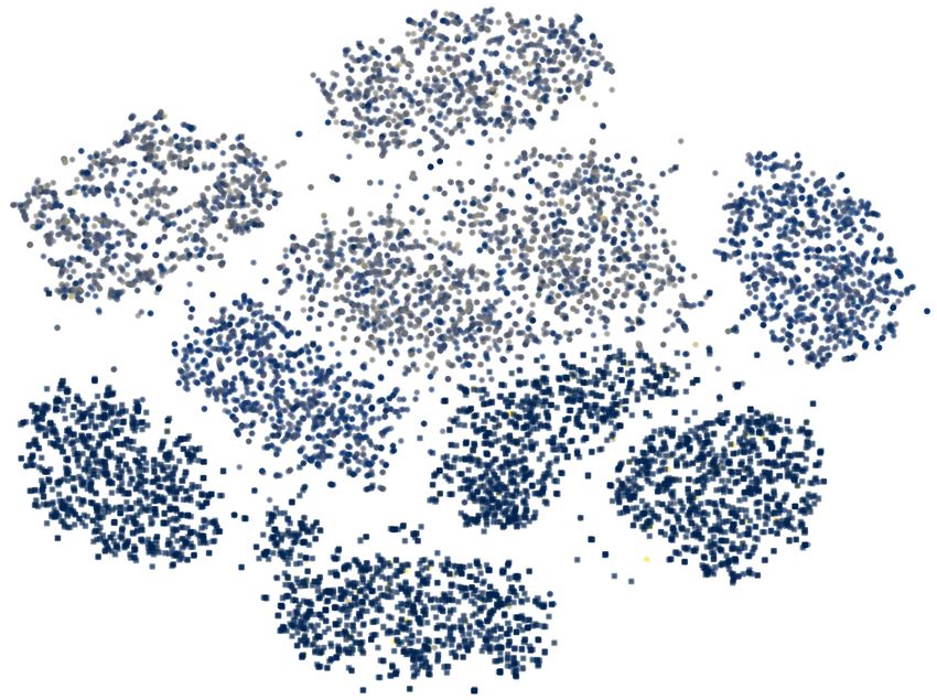
Published as a conference paper at ICLR 2022

sume that given z and c, the uncensored survival time follows the Weibull distribution given by
Weibull softplus z > βc , k , where softplus(x) = log (1 + exp(x)); k is the shape parameter; and
βc are cluster-specific survival parameters.   Note that we omitted the bias term βc,0 for the sake of
brevity. Observe that softplus z > βc corresponds to the scale parameter of the Weibull distribution.

We assume that the shape parameter k is global; however, an adaptation to cluster-specific parame-
ters, as proposed by Liverani et al. (2020), is straightforward. The Weibull distribution with
                                                                                            scale  λ
                                                                            k x k−1

                                                                                                x k
and shape k has the probability density function given by f (x; λ, k) = λ λ            exp − λ        ,
for x ≥ 0. Consequently, adjusting for right-censoring yields the following distribution:
        p(t|z, c; β, k) = f (t; λzc , k)δ S(t|z, c)1−δ
                            "      k−1                k !#δ "            k !#1−δ               (1)
                               k     t                   t                      t
                         =      z     z
                                              exp −       z
                                                                    exp −        z
                                                                                               ,
                              λc λc                     λc                    λc
                                                                        ∞
where β = {β1 , . . . , βK }; λzc = softplus z > βc ; and S(t|z, c) = t=t f (t; λzc , k) is the survival
                                                                     R

function. Henceforth, we will use p(t|z, c) as a shorthand notation for p(t|z, c; β, k). In this paper,
we only consider right-censoring; however, the proposed model can be extended to tackle other
forms of censoring.

Joint Probability Distribution Assuming Rthe generative process describedR PK above, the joint prob-
                                                   PK
ability of x and t can be written as p(x, t) = z c=1 p(x, t, z, c) = z c=1 p(x|t, z, c)p(t, z, c).
It is important to note that x and t are independent given z, so are x and c. Hence, we can rewrite
the joint probability of the data, also referred to as the likelihood function, given the parameters π,
µ, Σ, γ, β, k as
                                       Z X  K
         p (x, t; π, µ, Σ, γ, β, k) =          p(x|z; γ)p(t|z, c; β, k)p(z|c; µ, Σ)p(c; π),         (2)
                                        z c=1

where µ = {µ1 , ..., µK }, Σ = {Σ1 , ..., ΣK }, and β = {β1 , ..., βK }.

Evidence Lower Bound Given the data generating assumptions stated before, the objective is to
infer the parameters π, µ, Σ, γ, and β which better explain the covariates and survival outcomes
{xi , ti }N
          i=1 . Since the likelihood function in Equation 2 is intractable, we maximise a lower bound
of the log marginal probability of the data:

                                                      p(x|z; γ)p(t|z, c; β, k)p(z|c; µ, Σ)p(c; π)
  log p(x, t; π, µ, Σ, γ, β, k) ≥ Eq(z,c|x,t) log                                                   . (3)
                                                                      q(z, c|x, t)
We approximate the probability of the latent variables z and c given the observations with a varia-
tional distribution q(z, c|x, t) = q(z|x)q(c|z, t), where the first term is the encoder parameterised
by a neural network. The second term is equal to the true probability p(c|z, t):
                                            p(z, t|c)p(c)           p(t|z, c)p(z|c)p(c)
                q(c|z, t) = p(c|z, t) = PK                    = PK                         .          (4)
                                           c=1 p(z, t|c)p(c)       c=1 p(t|z, c)p(z|c)p(c)

Thus, the evidence lower bound (ELBO) can be written as
            L(x, t) = Eq(z|x)p(c|z,t) log p(x|z; γ) + Eq(z|x)p(c|z,t) log p(t|z, c; β, k)
                                                                                                     (5)
                     − DKL (q (z, c|x, t) k p (z, c; µ, Σ, π)) .
Of particular interest is the second term which encourages the model to maximise the probability of
observing the given survival outcome t under the variational distribution of the latent embeddings
and cluster assignments q(z, c|x, t). It can be then seen as a mixture of survival distributions, each
one assigned to one cluster. The ELBO can be approximated using the stochastic gradient variational
Bayes (SGVB) estimator (Kingma & Welling, 2014) to be maximised efficiently using stochastic
gradient descent. For the complete derivation, we refer to Appendix D.

Missing Survival Time The hard cluster assignments can be computed from the distribution
p(c|z, t) of Equation 4. However, the survival times may not be observable at test-time; whereas our
derivation of the distribution p(c|z, t) depends on p(t|z, c). Therefore, when the survival time of an
individual is unknown, using the Bayes’ rule we instead compute p(c|z) = PKp(z|c)p(c)
                                                                                    p(z|c)p(c)
                                                                                               .
                                                                                  c=1

                                                   4
Published as a conference paper at ICLR 2022

4   E XPERIMENTAL S ETUP
Datasets We evaluate VaDeSC on a range of synthetic, semi-synthetic (survMNIST; Pölsterl
(2019)), and real-world survival datasets with varying numbers of data points, explanatory vari-
ables, and fractions of censored observations (see Table 2). In particular, real-world clinical datasets
include two benchmarks common in the survival analysis literature, namely SUPPORT (Knaus et al.,
1995) and FLChain (Kyle et al., 2006; Dispenzieri et al., 2012); an observational cohort of pediatric
patients undergoing chronic hemodialysis (Hemodialysis; Gotta et al. (2021)); an observational co-
hort of high-grade glioma patients (HGG); and an aggregation of several computed tomography
(CT) image datasets acquired from patients diagnosed with non-small cell lung cancer (NSCLC;
Aerts et al. (2019); Bakr et al. (2017); Clark et al. (2013); Weikert et al. (2019)). Detailed descrip-
tion of the datasets and preprocessing can be found in Appendices E and G. For (semi-)synthetic
data, we focus on the clustering performance of the considered methods; whereas for real-world
data, where the true cluster structure is unknown, we compare time-to-event predictions. In addi-
tion, we provide an in-depth cluster analysis for the NSCLC (see Section 5.3) and Hemodialysis (see
Appendix H.8) datasets.

Table 2: Summary of the datasets. Here, N is the total number of data points, D is the number of
explanatory variables, K is the number of clusters if known. We report the percentage of censored
observations and whether the cluster sizes are balanced if known.

      Dataset            N         D      % censored     Data type    K     Balanced?     Section
      Synthetic        60,000    1,000        30          Tabular     3         Y         5.1, H.2
      survMNIST        70,000   28×28         52          Image       5         N         5.1, H.6
      SUPPORT          9,105       59         32          Tabular     —         —           5.2
      FLChain          6,524        7         70          Tabular     —         —           H.7
      HGG               453       147         25          Tabular     —         —           5.2
      Hemodialysis     1,493       57         91          Tabular     —         —         5.2, H.8
      NSCLC             961     64×64         33          Image       —         —         5.3, H.9

Baselines & Ablations We compare our method to several well-established baselines: the semi-
supervised clustering (SSC; Bair & Tibshirani (2004)), survival cluster analysis (Chapfuwa et al.,
2020), and deep survival machines (Nagpal et al., 2021a). For the sake of fair comparison, in SCA
we truncate the Dirichlet process at the true number of clusters if known. For all neural network
techniques, we use the same encoder architectures and numbers of latent dimensions. Although the
profile regression approach of Liverani et al. (2020) is closely related to ours, it is not scalable to
large unstructured datasets, such as survMNIST and NSCLC, since it relies on MCMC methods for
Bayesian inference and is not parameterised by neural networks. Therefore, a full-scale comparison
is impossible due to computational limitations. Appendix H.3 contains a ‘down-scaled’ experiment
with the profile regression on synthetic data. Additionally, we consider k-means and regularised
Cox PH and Weibull AFT models (Simon et al., 2011) as naı̈ve baselines. For the VaDeSC, we
perform several ablations: (i) removing the Gaussian mixture prior and performing post hoc k-
means clustering on latent representations learnt by a VAE with an auxiliary Weibull survival loss
term, which is similar to the deep survival analysis (DSA; Ranganath et al. (2016)) combined with
k-means; (ii) training a completely unsupervised version without modelling the survival, which is
similar to VaDE (Jiang et al., 2017); and (iii) predicting cluster assignments when the survival time
is unobserved. Appendix G contains further implementation details.

Evaluation We evaluate the clustering performance of models, when possible, in terms of accu-
racy (ACC), normalised mutual information (NMI), and adjusted Rand index (ARI). For the time-
to-event predictions, we evaluate the ability of methods to rank individuals by their risk using the
concordance index (CI; Raykar et al. (2007)). Predicted median survival times are evaluated using
the relative absolute error (RAE; Yu et al. (2011)) and calibration slope (CAL), as implemented by
Chapfuwa et al. (2020). We report RAE on both non-censored (RAEnc ) and censored (RAEc ) data
points (see Equations 14 and 15 in Appendix F). The relative absolute error quantifies the relative
deviation of median predictions from the observed survival times; while the calibration slope in-
dicates whether a model tends to under- or overestimate risk on average. For the (semi-)synthetic
datasets we average all results across independent simulations, i.e. dataset replicates; while for the
real-world data we use the Monte Carlo cross-validation procedure.

                                                   5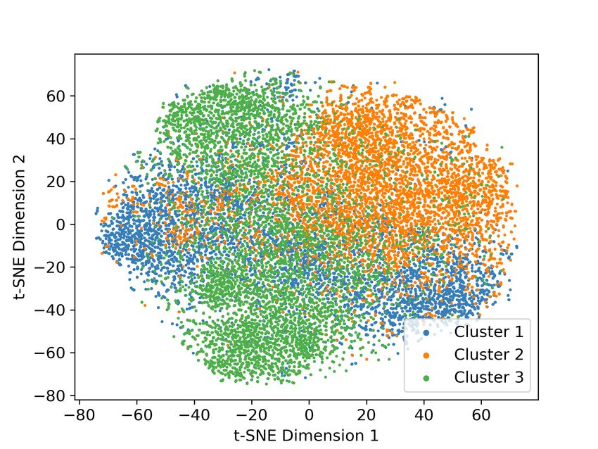
Published as a conference paper at ICLR 2022

5     R ESULTS

5.1   C LUSTERING

We first compare clustering performance on the nonlinear (semi-)synthetic data. Table 3 shows
the results averaged across several simulations. In addition to the clustering, we evaluate the con-
cordance index to verify that the methods can adequately model time-to-event in these datasets.
Training set results are reported in Table 12 in Appendix H.
As can be seen, in both problems, VaDeSC outperforms other models in terms of clustering and
achieves performance comparable to SCA and DSM w.r.t. the CI. Including survival times appears to
help identify clusters since the completely unsupervised VaDE achieves significantly worse results.
It is also assuring that the model is able to predict clusters fairly well even when the survival time is
not given at test time (“w/o t”). Furthermore, performing k-means clustering in the latent space of a
VAE with the Weibull survival loss (“VAE + Weibull”) clearly does not lead to the identification of
the correct clusters. In both datasets, k-means on VAE representations yields almost no improvement
over k-means on raw features. This suggests that the Gaussian mixture structure incorporated in the
generative process of VaDeSC plays an essential role in inferring clusters.
Interestingly, while SCA and DSM achieve good results on survMNIST, both completely fail to iden-
tify clusters correctly on synthetic data, for which the generative process is very similar to the one
assumed by VaDeSC. In the synthetic data, the clusters do not have prominently different survival
distributions (see Appendix E.1); they are rather characterised by different associations between the
covariates and survival times — whereas the two baseline methods tend to discover clusters with
disparate survival distributions. The SSC offers little to no gain over the conventional k-means per-
formed on the complete feature set. Last, we note that in both datasets VaDeSC has a significantly
better CI than the Cox PH model likely due to its ability to capture nonlinear relationships between
the covariates and outcome.
Figure 4 provides a closer inspection of the clustering and latent representations on survMNIST
data. It appears that SCA and DSM, as expected, fail to discover clusters with similar Kaplan–
Meier (KM) curves and have a latent space that is driven purely by survival time. While the VAE +
Weibull model learns representations driven by both the explanatory variables (digits in the images)
and survival time, the post hoc k-means clustering fails at identifying the true clusters. By contrast,
VaDeSC is capable of discovering clusters with even minor differences in KM curves and learns

Table 3: Test set clustering performance on synthetic and survMNIST data. “VAE + Weibull”
corresponds to an ablation of VaDeSC w/o the Gaussian mixture prior. “w/o t” corresponds to the
cluster assignments made by VaDeSC when the survival time is not given. Averages and standard
deviations are reported across 5 and 10 independent simulations, respectively. Best results are shown
in bold, second best – in italic.

         Dataset         Method               ACC           NMI           ARI            CI
                         k-means           0.44±0.04     0.06±0.04     0.05±0.03         —
                         Cox PH                —             —             —         0.77±0.02
                         SSC               0.45±0.03     0.08±0.04     0.06±0.02         —
                         SCA               0.45±0.09     0.05±0.05     0.04±0.05     0.82±0.02
         Synthetic       DSM               0.37±0.02     0.01±0.00     0.01±0.00     0.76±0.02
                         VAE + Weibull     0.46±0.06     0.09±0.04     0.09±0.04     0.71±0.02
                         VaDE              0.74±0.21     0.53±0.12     0.55±0.20         —
                         VaDeSC (w/o t)    0.88±0.03     0.60±0.07     0.67±0.07
                                                                                     0.84±0.02
                         VaDeSC (ours)     0.90±0.02     0.66±0.05     0.73±0.05
                         k-means           0.49±0.06     0.31±0.04     0.22±0.04         —
                         Cox PH                —             —             —         0.74±0.04
                         SSC               0.49±0.06     0.31±0.04     0.22±0.04         —
                         SCA               0.56±0.09     0.46±0.06     0.33±0.10     0.79±0.06
         survMNIST       DSM               0.54±0.11     0.40±0.16     0.31±0.14     0.79±0.05
                         VAE + Weibull     0.49±0.05     0.32±0.05     0.24±0.05     0.76±0.07
                         VaDE              0.47±0.07     0.38±0.08     0.24±0.08         —
                         VaDeSC (w/o t)    0.57±0.09     0.51±0.09     0.37±0.10
                                                                                     0.80±0.05
                         VaDeSC (ours)     0.58±0.10     0.55±0.11     0.39±0.11

                                                   6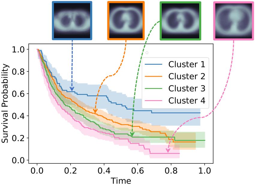
Published as a conference paper at ICLR 2022

  (a) Ground truth    (b) VAE + Weibull        (c) SCA               (d) DSM        (e) VaDeSC (ours)

Figure 4: Cluster-specific Kaplan–Meier (KM) curves (top) and t-SNE visualisation of latent rep-
resentations (bottom), coloured according to survival times (yellow and blue correspond to higher
and lower survival times, respectively), learnt by different models (b-e) from one replicate of the
survMNIST dataset. Panel (a) shows KM curves of the ground truth clusters. Plots were generated
using 10,000 data points randomly sampled from the training set; similar results were observed on
the test set.

Table 4: Test set time-to-event performance on SUPPORT, HGG, and Hemodialysis datasets. Aver-
ages and standard deviations are reported across 5 independent train-test splits.

         Dataset          Method               CI          RAEnc        RAEc          CAL
                          Cox PH           0.84±0.01         —            —            —
                          Weibull AFT      0.84±0.01     0.62±0.01    0.13±0.01    1.27±0.02
                          SCA              0.83±0.02     0.78±0.13    0.06±0.04    1.74±0.52
         SUPPORT
                          DSM              0.87±0.01     0.56±0.02    0.13±0.04    1.43±0.07
                          VAE + Weibull    0.84±0.01     0.56±0.02    0.20±0.02    1.28±0.04
                          VaDeSC (ours)    0.85±0.01     0.53±0.02    0.23±0.05    1.24±0.05
                          Cox PH           0.74±0.05         —            —            —
                          Weibull AFT      0.74±0.05     0.56±0.04    0.14±0.09    1.16±0.10
                          SCA              0.63±0.08     0.97±0.05    0.00±0.00    2.59±1.70
         HGG
                          DSM              0.75±0.04     0.57±0.05    0.18±0.07    1.09±0.08
                          VAE + Weibull    0.75±0.05     0.52±0.06    0.12±0.07    1.14±0.11
                          VaDeSC (ours)    0.74±0.05     0.53±0.06    0.13±0.07    1.12±0.09
                          Cox PH           0.83±0.04         —            —            —
                          Weibull AFT      0.83±0.05     0.81±0.03    0.01±0.00    4.46±0.59
                          SCA              0.75±0.05     0.86±0.07    0.02±0.02    7.93±3.22
         Hemodialysis
                          DSM              0.80±0.06     0.85±0.08    0.02±0.04    8.23±4.28
                          VAE + Weibull    0.77±0.06     0.80±0.06    0.02±0.01    4.49±0.75
                          VaDeSC (ours)    0.80±0.05     0.78±0.05    0.01±0.00    3.74±0.58

representations that clearly reflect the covariate and survival variability. Similar differences can be
observed for the synthetic data (see Appendix H.2).

5.2   T IME - TO - EVENT P REDICTION

We now assess time-to-event prediction on clinical data. As these datasets do not have ground truth
clustering labels, we do not evaluate the clustering performance. However, for Hemodialysis, we
provide an in-depth qualitative assessment of the learnt clusters in Appendix H.8.
Table 4 shows the time-to-event prediction performance on SUPPORT, HGG, and Hemodialysis.
Results for FLChain are reported in Appendix H.7 and yield similar conclusions. Surprisingly, SCA
often has a considerable variance w.r.t. the calibration slope, sometimes yielding badly calibrated
predictions. Note, that for SCA and DSM, the results differ from those reported in the original
papers likely due to a different choice of encoder architectures and numbers of latent dimensions. In
general, these results are promising and suggest that VaDeSC remains competitive at time-to-event
modelling, offers overall balanced predictions, and is not prone to extreme overfitting even when
applied to simple clinical datasets that are low-dimensional or contain few non-censored patients.

                                                  7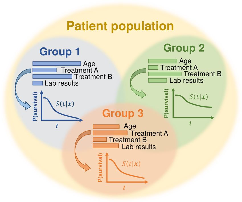
Published as a conference paper at ICLR 2022

5.3   A PPLICATION TO C OMPUTED T OMOGRAPHY DATA

We further demonstrate the viability of our model in a real-world application using a collection of
several CT image datasets acquired from NSCLC patients (see Appendix E). The resulting dataset
poses two major challenges. The first one is the high variability among samples, mainly due to
disparate lung tumour locations. In addition, several demographic characteristics, such as patient’s
age, sex, and weight, might affect both the CT scans and survival outcome. Thus, a representation
learning model that captures cluster-specific associations between medical images and survival times
could be highly beneficial to both explore the sources of variability in this dataset and to understand
the different generative mechanisms of the survival outcome. The second challenge is the modest
dataset size (N = 961). To this end, we leverage image augmentation during neural network training
(Perez & Wang, 2017) to mitigate spurious associations between survival outcomes and clinically
irrelevant CT scan characteristics (see Appendix G).
We compare our method to the DSM, omitting the SCA, which seems to yield results similar to
the latter. As well-established time-to-event prediction baselines, we fit Cox PH and Weibull AFT
models on radiomics features. The latter are extracted using manual pixel-wise tumour segmentation
maps, which are time-consuming and expensive to obtain. Note that neither DSM nor VaDeSC
requires segmentation as an input. Table 5 shows the time-to-event prediction results. Interestingly,
DSM and VaDeSC achieve performance comparable to the radiomics-based models, even yielding
a slightly better calibration on average. This suggests that laborious manual tumour segmentation is
not necessary for survival analysis on CT scans. Similarly to tabular clinical datasets (see Table 4),
DSM and VaDeSC have comparable performance. Therefore, we investigate cluster assignments
qualitatively to highlight the differences between the two methods.

Table 5: Test set time-to-event prediction performance on NSCLC data. For Cox PH and Weibull
AFT, radiomics features were extracted using tumour segmentation maps. Averages and standard
deviations are reported across 100 independent train-test splits, stratified by survival time.

            Method                          CI            RAEnc       RAEc         CAL
            Radiomics + Cox PH          0.60±0.02           —           —           —
            Radiomics + Weibull AFT     0.60±0.02       0.70±0.02   0.45±0.03   1.26±0.04
            DSM                         0.59±0.04       0.72±0.03   0.34±0.06   1.24±0.07
            VaDeSC (ours)               0.60±0.02       0.71±0.03   0.35±0.05   1.21±0.05

In Figure 5, we plot the KM curves and corresponding centroid CT images for the clusters discov-
ered by DSM and VaDeSC on one train-test split. By performing several independent experiments
(see Appendix H.10), we observe that both methods discover patient groups with different empirical
survival time distributions. However, in contrast to DSM, VaDeSC clusters are consistently associ-
ated with the tumour location. On the contrary, the centroid CT images of the DSM clusters show

                     (a) DSM                                         (b) VaDeSC (ours)

Figure 5: Cluster-specific Kaplan–Meier curves and corresponding centroid CT images, computed
by averaging all samples assigned to each cluster by (a) DSM and (b) VaDeSC on the NSCLC data.

                                                    8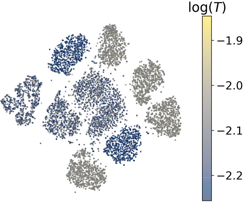
Published as a conference paper at ICLR 2022

Table 6: Cluster-specific statistics for a few demographic and clinical variables (not used during
training) from the NSCLC dataset for DSM and VaDeSC. T. Vol. stands for the tumour volume; M1
denotes spread of cancer to distant organs and tissues; and ≥ T3 denotes a tumour stage of at least
3. Kruskal-Wallis H-test p-values are reported at the significance levels of 0.001, 0.01, and 0.05.

                                        DSM                         VaDeSC (ours)
            Variable
                           1     2     3    4     p-val.    1     2    3    4     p-val.
            T. Vol., cm3   23    39    38 51      ≤ 1e-3    43    36 40     63    ≤ 5e-2
            Age, yrs       67    68    68 69       0.11     62    69 67     70    ≤ 1e-3
            Female, %      29    30    26 21       0.3      36    19 38     23    ≤ 1e-3
            Smoker, %      84   100    80 89       0.9      67    94 87 100        0.12
            M1, %          40    55    16 42       0.4      20    45 44     45     0.2
            ≥ T3, %        27    12    23 32       0.2      10    29 35     31     0.7

no visible difference. This is further demonstrated in Figure 6, where we generated several CT scans
for each cluster by sampling from the multivariate Gaussian distribution in the latent space of the
VaDeSC. We observe a clear association with tumour location, as clusters 1 () and 3 () corre-
spond to the upper section of the lungs. Indeed, multiple studies have suggested a higher five-year
survival rate in patients with the tumour in the upper lobes (Lee et al., 2018). It is also interesting
                                                  to observe the amount of variability within each
                                                  cluster: every generated scan is characterised by a
                                                  unique lung shape and tumour size. Since DSM is
                                                  not a generative model, we instead plot the original
                                                  samples assigned to each cluster by DSM in Ap-
                                                  pendix H.9. Finally, in Table 6 we compute cluster-
                                                  specific statistics for a few important demographic
                                                  and clinical variables (Etiz et al., 2002; Agarwal
                                                  et al., 2010; Bhatt et al., 2014). We observe that
                                                  VaDeSC tends to discover clusters with more dis-
                                                  parate characteristics and is thus able to stratify
                                                  patients not only by risk but also by clinical con-
                                                  ditions. Overall, the results above agree with our
Figure 6: CT images generated by (i) sampling
                                                  findings on (semi-)synthetic data: VaDeSC identi-
latent representations from the Gaussian mix-
                                                  fies clusters informed by both the covariates and
ture learnt by VaDeSC and (ii) decoding rep-
                                                  survival outcomes, leading to a stratification very
resentations using the decoder network.
                                                  different from previous approaches.

6   C ONCLUSION
In this paper, we introduced a novel deep probabilistic model for clustering survival data. In contrast
to existing approaches, our method can retrieve clusters driven by both the explanatory variables
and survival information and it can be trained efficiently in the framework of stochastic gradient
variational inference. Empirically, we showed that our model offers an improvement in clustering
performance compared to the related work while staying competitive at time-to-event modelling.
We also demonstrated that our method identifies meaningful clusters from a challenging medical
imaging dataset. The analysis of these clusters provides interesting insights that could be useful for
clinical decision-making. To conclude, the proposed VaDeSC model offers a holistic perspective on
clustering survival data by learning structured representations which reflect the covariates, outcomes,
and varying relationships between them.

Limitations & Future Work The proposed model has a few limitations. It requires fixing a
number of mixture components a priori since global parameters are not treated in a fully Bayesian
manner, as opposed to the profile regression. Although the obtained cluster assignments can be
explained post hoc, the relationship between the raw features and survival outcomes remains unclear.
Thus, further directions of work include (i) improving the interpretability of our model to facilitate
its application in the medical domain and (ii) a fully Bayesian treatment of global parameters. In-
depth interpretation of the clusters we found in clinical datasets is beyond the scope of this paper,
but we plan to investigate these clusters together with our clinical collaborators in follow-up work.

                                                  9
Published as a conference paper at ICLR 2022

ACKNOWLEDGEMENTS
We thank Alexandru T, ifrea, Nicolò Ruggeri, and Kieran Chin-Cheong for valuable discussion and
comments and Dr. Silvia Liverani, Paidamoyo Chapfuwa, and Chirag Nagpal for sharing the code.
Ričards Marcinkevičs is supported by the SNSF grant #320038189096. Laura Manduchi is sup-
ported by the PHRT SHFN grant #1-000018-057: SWISSHEART.

E THICS S TATEMENT
The in-house PET/CT and HGG data were acquired at the University Hospital Basel and Univer-
sity Hospital Zürich, respectively, and retrospective, observational studies were approved by local
ethics committees (Ethikkommission Nordwest- und Zentralschweiz, no. 2016-01649; Kantonale
Ethikkommission Zürich, no. PB-2017-00093).

R EPRODUCIBILITY S TATEMENT
To ensure the reproducibility of this work several measures were taken. The experimental setup
is outlined in Section 4. Appendix E details benchmarking datasets and simulation procedures.
Appendix F defines metrics used for model comparison. Appendix G contains data preprocess-
ing, architecture, and hyperparameter tuning details. For the computed tomography data we as-
sess the stability of the obtained results in Appendix H.10. Most datasets used for compari-
son are either synthetic or publicly available. HGG, Hemodialysis, and in-house PET/CT data
could not be published due to medical confidentiality. The code is publicly available at https:
//github.com/i6092467/vadesc.

R EFERENCES
M. Abadi, A. Agarwal, P. Barham, E. Brevdo, Z. Chen, C. Citro, G. S. Corrado, A. Davis, J. Dean,
 M. Devin, S. Ghemawat, I. Goodfellow, A. Harp, G. Irving, M. Isard, Y. Jia, R. Jozefow-
 icz, L. Kaiser, M. Kudlur, J. Levenberg, D. Mané, R. Monga, S. Moore, D. Murray, C. Olah,
 M. Schuster, J. Shlens, B. Steiner, I. Sutskever, K. Talwar, P. Tucker, V. Vanhoucke, V. Va-
 sudevan, F. Viégas, O. Vinyals, P. Warden, M. Wattenberg, M. Wicke, Y. Yu, and X. Zheng.
 TensorFlow: Large-scale machine learning on heterogeneous systems, 2015. URL http:
 //tensorflow.org/.
H. J. W. L. Aerts, E. R. Velazquez, R. Leijenaar, C. Parmar, P. Grossmann, S. Cavalho, J. Bussink,
  R. Monshouwer, B. Haibe-Kains, D. Rietveld, F. Hoebers, M. Rietbergen, C. R. Leemans,
  A. Dekker, J. Quackenbush, R. Gillies, and P. Lambin. Decoding tumour phenotype by non-
  invasive imaging using a quantitative radiomics approach. Nature Communications, 5, 2014.
H. J. W. L. Aerts, E. Rios Velazquez, R. T. H. Leijenaar, C. Parmar, P. Grossmann, S. Carvalho,
  J. Bussink, R. Monshouwer, B. Haibe-Kains, D. Rietveld, F. Hoebers, M. M. Rietbergen, C. R.
  Leemans, A. Dekker, J. Quackenbush, R. J. Gillies, and P. Lambin. Data from NSCLC-radiomics-
  genomics, 2015. URL https://wiki.cancerimagingarchive.net/x/GAL1.
H. J. W. L. Aerts, L. Wee, E. Rios Velazquez, R. T. H. Leijenaar, C. Parmar, P. Grossmann, S. Car-
  valho, J. Bussink, R. Monshouwer, B. Haibe-Kains, D. Rietveld, F. Hoebers, M. M. Rietbergen,
  C. R. Leemans, A. Dekker, J. Quackenbush, R. J. Gillies, and P. Lambin. Data from NSCLC-
  radiomics, 2019. URL https://wiki.cancerimagingarchive.net/x/FgL1.
M. Agarwal, G. Brahmanday, G. W. Chmielewski, R. J. Welsh, and K. P. Ravikrishnan. Age, tumor
 size, type of surgery, and gender predict survival in early stage (stage I and II) non-small cell lung
 cancer after surgical resection. Lung Cancer, 68(3):398–402, 2010.
E. Ahlqvist, P. Storm, A. Käräjämäki, M. Martinell, M. Dorkhan, A. Carlsson, P. Vikman, R. B.
  Prasad, D. M. Aly, P. Almgren, Y. Wessman, N. Shaat, P. Spégel, H. Mulder, E. Lindholm,
  O. Melander, O. Hansson, U. Malmqvist, Å. Lernmark, K. Lahti, T. Forsén, T. Tuomi, A. H.
  Rosengren, and L. Groop. Novel subgroups of adult-onset diabetes and their association with
  outcomes: a data-driven cluster analysis of six variables. The Lancet Diabetes & Endocrinology,
  6(5):361–369, 2018.

                                                  10
Published as a conference paper at ICLR 2022
S. Amaral, W. Hwang, B. Fivush, A. Neu, D. Frankenfield, and S. Furth. Serum albumin level
and risk for mortality and hospitalization in adolescents on hemodialysis. Clinical journal of the
American Society of Nephrology, 3(3):759–767, 2008.
E. Bair and R. Tibshirani. Semi-supervised methods to predict patient survival from gene expression
data. PLoS Biology, 2(4):e108, 2004.
S. Bakr, O. Gevaert, S. Echegaray, K. Ayers, M. Zhou, M. Shafiq, H. Zheng, W. Zhang, A. Le-
ung, M. Kadoch, J. Shrager, A. Quon, D. Rubin, S. Plevritis, and S. Napel. Data for NSCLC
radiogenomics collection, 2017. URL https://wiki.cancerimagingarchive.net/
x/W4G1AQ.
S. Bakr, O. Gevaert, S. Echegaray, K. Ayers, M. Zhou, M. Shafiq, H. Zheng, J. Anthony B.,
W. Zhang, A. N. C. Leung, M. Kadoch, C. D. Hoang, J. Shrager, A. Quon, D. L. Rubin, S. K.
Plevritis, and S. Napel. A radiogenomic dataset of non-small cell lung cancer. Scientific Data, 5
(1), 2018.
G. A. Bello, T. J. W. Dawes, J. Duan, C. Biffi, A. de Marvao, L. S. G. Howard, J. S. R. Gibbs, M. R.
Wilkins, S. A. Cook, D. Rueckert, and D. P. O’Regan. Deep learning cardiac motion analysis for
human survival prediction. Nature machine intelligence, 1:95–104, 2019.
A. Ben-Hur, A. Elisseeff, and I. Guyon. A stability based method for discovering structure in
clustered data. Pacific Symposium on Biocomputing. Pacific Symposium on Biocomputing, pp.
6–17, 2002.
V. R. Bhatt, R. Batra, P. T. Silberstein, F. R. Loberiza, and A. K. Ganti. Effect of smoking on sur-
vival from non-small cell lung cancer: a retrospective Veterans’ Affairs Central Cancer Registry
(VACCR) cohort analysis. Medical Oncology, 32(1), 2014.
J. Buckley and I. James. Linear regression with censored data. Biometrika, 66(3):429–436, 1979.
J. C. Buckner. Factors influencing survival in high-grade gliomas. Seminars in Oncology, 30:10–14,
2003.
P. Chapfuwa, C. Tao, C. Li, C. Page, B. Goldstein, L. C. Duke, and R. Henao. Adversarial time-
to-event modeling. In Proceedings of the 35th International Conference on Machine Learning,
volume 80, pp. 735–744. PMLR, 2018.
P. Chapfuwa, C. Li, N. Mehta, L. Carin, and R. Henao. Survival cluster analysis. In Proceedings of
the ACM Conference on Health, Inference, and Learning, pp. 60–68. Association for Computing
Machinery, 2020.
T. Chen and C. Guestrin. XGBoost: A scalable tree boosting system. In Proceedings of the 22nd
ACM SIGKDD International Conference on Knowledge Discovery and Data Mining, pp. 785–
794. ACM, 2016.
K. Clark, B. Vendt, K. Smith, J. Freymann, J. Kirby, P. Koppel, S. Moore, S. Phillips, D. Maf-
fitt, M. Pringle, L. Tarbox, and F. Prior. The cancer imaging archive (TCIA): Maintaining and
operating a public information repository. Journal of Digital Imaging, 26(6):1045–1057, 2013.
F. S. Collins and H. Varmus. A new initiative on precision medicine. New England Journal of
Medicine, 372(9):793–795, 2015.
D. R. Cox. Regression models and life-tables. Journal of the Royal Statistical Society: Series B
(Methodological), 34(2):187–202, 1972.
D. G. Altman. Analysis of survival times. In Practical Statistics for Medical Research, chapter 13,
pp. 365–395. Chapman and Hall/CRC Texts in Statistical Science Series, 2020.
J. Daugirdas. Second generation logarithmic estimates of single-pool variable volume Kt/V: an
analysis of error. Journal of the American Society of Nephrology : JASN, 4(5):1205–1213, 1993.
J. Daugirdas and D. Schneditz. Overestimation of hemodialysis dose depends on dialysis efficiency
by regional blood flow but not by conventional two pool urea kinetic analysis. ASAIO journal, 41
(3):M719–M724, 1995.
11Published as a conference paper at ICLR 2022
C. Davidson-Pilon, J. Kalderstam, N. Jacobson, S. Reed, B. Kuhn, P. Zivich, M. Williamson, J. K.
Abdeali, D. Datta, A. Fiore-Gartland, A. Parij, D. Wilson, Gabriel, L. Moneda, A. Moncada-
Torres, K. Stark, H. Gadgil, Jona, K. Singaravelan, L. Besson, M. Sancho Peña, S. Anton,
A. Klintberg, J. Growth, J. Noorbakhsh, M. Begun, R. Kumar, S. Hussey, S. Seabold, and D. Gol-
land. lifelines: v0.25.9, 2021. URL https://doi.org/10.5281/zenodo.4505728.
N. Dilokthanakul, P. A. M. Mediano, M. Garnelo, M. C. H. Lee, H. Salimbeni, K. Arulkumaran,
and M. Shanahan. Deep unsupervised clustering with Gaussian mixture variational autoencoders,
2016. arXiv:1611.02648.
A. Dispenzieri, J. A. Katzmann, R. A. Kyle, D. R. Larson, T. M. Therneau, C. L. Colby, R. J. Clark,
G. P. Mead, S. Kumar, L. J. Melton, and S. V. Rajkumar. Use of nonclonal serum immunoglobulin
free light chains to predict overall survival in the general population. Mayo Clinic Proceedings,
87(6):517–523, 2012.
D. Etiz, L. B. Marks, S.-M. Zhou, G. C. Bentel, R. Clough, M. L. Hernando, and P. A. Lind.
Influence of tumor volume on survival in patients irradiated for non-small-cell lung cancer. Inter-
national Journal of Radiation Oncology, Biology, Physics, 53(4):835–846, 2002.
D. Faraggi and R. Simon. A neural network model for survival data. Statistics in Medicine, 14(1):
73–82, 1995.
V. T. Farewell. The use of mixture models for the analysis of survival data with long-term survivors.
Biometrics, 38(4):1041–1046, 1982.
D. A. Fenstermacher, R. M. Wenham, D. E. Rollison, and W. S. Dalton. Implementing personalized
medicine in a cancer center. The Cancer Journal, 17(6):528–536, 2011.
R. Foley, P. Parfrey, J. Harnett, G. M. Kent, D. Murray, and P. Barre. Hypoalbuminemia, cardiac
morbidity, and mortality in end-stage renal disease. Journal of the American Society of Nephrol-
ogy : JASN, 7 5:728–36, 1996.
O. Gevaert, J. Xu, C. D. Hoang, A. N. Leung, Y. Xu, A. Quon, D. L. Rubin, S. Napel, and S. K.
Plevritis. Non–small cell lung cancer: Identifying prognostic imaging biomarkers by leveraging
public gene expression microarray data—methods and preliminary results. Radiology, 264(2):
387–396, 2012.
M. Goldstein, X. Han, A. Puli, A. Perotte, and R. Ranganath. X-CAL: Explicit calibration for
survival analysis. Advances in neural information processing systems, 33:18296–18307, 2020.
V. Gotta, O. Marsenic, and M. Pfister. Age- and weight-based differences in haemodialysis prescrip-
tion and delivery in children, adolescents and young adults. Nephrology Dialysis Transplantation,
33:1649–1660, 2018.
V. Gotta, O. Marsenic, and M. Pfister. Understanding urea kinetic factors that enhance personalized
hemodialysis prescription in children. ASAIO Journal, 66:115 – 123, 2019a.
V. Gotta, M. Pfister, and O. Marsenic. Ultrafiltration rates in children on chronic hemodialysis
routinely exceed weight based adult limit. Hemodialysis International, 23, 2019b.
V. Gotta, G. Tancev, O. Marsenic, J. E. Vogt, and M. Pfister. Identifying key predictors of mortality
in young patients on chronic haemodialysis – a machine learning approach. Nephrology, dialy-
sis, transplantation : official publication of the European Dialysis and Transplant Association -
European Renal Association, 2020.
V. Gotta, O. Marsenic, A. Atkinson, and M. Pfister. Hemodialysis (HD) dose and ultrafiltration rate
are associated with survival in pediatric and adolescent patients on chronic hd—a large observa-
tional study with follow-up to young adult age. Pediatric Nephrology, pp. 1–12, 2021.
C. Haarburger, P. Weitz, O. Rippel, and D. Merhof. Image-based survival prediction for lung cancer
patients using CNNs. In 2019 IEEE 16th International Symposium on Biomedical Imaging (ISBI
2019). IEEE, 2019.
12Published as a conference paper at ICLR 2022
H. Ishwaran, U. B. Kogalur, E. H. Blackstone, and M. S. Lauer. Random survival forests. Annals of
Applied Statistics, 2(3):841–860, 2008.
R. A. Jacobs, M. I. Jordan, S. J. Nowlan, and G. E. Hinton. Adaptive mixtures of local experts.
Neural Computation, 3(1):79–87, 1991.
Z. Jiang, Y. Zheng, H. Tan, B. Tang, and H. Zhou. Variational deep embedding: An unsupervised
and generative approach to clustering. In Proceedings of the 26th International Joint Conference
on Artificial Intelligence, pp. 1965–1972. AAAI Press, 2017.
M. J. Johnson, D. K. Duvenaud, A. Wiltschko, R. P. Adams, and S. R. Datta. Composing graphical
models with neural networks for structured representations and fast inference. In Advances in
Neural Information Processing Systems, volume 29, pp. 2946–2954. Curran Associates, Inc.,
2016.
J. L. Katzman, U. Shaham, A. Cloninger, J. Bates, T. Jiang, and Y. Kluger. DeepSurv: Personalized
treatment recommender system using a Cox proportional hazards deep neural network. BMC
Medical Research Methodology, 18(1), 2018.
D. P. Kingma and M. Welling. Auto-encoding variational Bayes. In 2nd International Conference
on Learning Representations, 2014.
W. A. Knaus, F. E. Harrell, J. Lynn, L. Goldman, R. S. Phillips, A. F. Connors, N. V. Dawson, W. J.
Fulkerson, R. M. Califf, N. Desbiens, P. Layde, R. K. Oye, P. E. Bellamy, R. B. Hakim, and
D. P. Wagner. The SUPPORT prognostic model: Objective estimates of survival for seriously ill
hospitalized adults. Annals of Internal Medicine, 122(3):191–203, 1995.
H. Kvamme, Ø. Borgan, and I. Scheel. Time-to-event prediction with neural networks and Cox
regression. Journal of Machine Learning Research, 20(129):1–30, 2019.
R. A. Kyle, T. M. Therneau, S. V. Rajkumar, D. R. Larson, M. F. Plevak, J. R. Offord, A. Dispenzieri,
J. A. Katzmann, and L. J. Melton. Prevalence of monoclonal gammopathy of undetermined
significance. New England Journal of Medicine, 354(13):1362–1369, 2006.
T. Lange, V. Roth, M. L. Braun, and J. M. Buhmann. Stability-based validation of clustering solu-
tions. Neural Computation, 16:1299–1323, 2004.
Y. LeCun, C. Cortes, and C. J. Burges. MNIST handwritten digit database. ATT Labs, 2, 2010. URL
http://yann.lecun.com/exdb/mnist.
H. W. Lee, C.-H. Lee, and Y. S. Park. Location of stage I-III non-small cell lung cancer and survival
rate: Systematic review and meta-analysis. Thoracic Cancer, 9(12):1614–1622, 2018.
J. L. Lehr and P. Capek. Histogram equalization of CT images. Radiology, 154(1):163–169, 1985.
S. Liverani, D. I. Hastie, L. Azizi, M. Papathomas, and S. Richardson. PReMiuM: An R package
for profile regression mixture models using Dirichlet processes. Journal of Statistical Software,
64(7), 2015.
S. Liverani, L. Leigh, I. L. Hudson, and J. E. Byles. Clustering method for censored and collinear
survival data. Computational Statistics, 2020.
S. M. Lundberg and S.-I. Lee. A unified approach to interpreting model predictions. In Advances in
Neural Information Processing Systems 30, pp. 4765–4774. Curran Associates, Inc., 2017.
S. M. Lundberg, G. Erion, H. Chen, A. DeGrave, J. M. Prutkin, B. Nair, R. Katz, J. Himmelfarb,
N. Bansal, and S.-I. Lee. From local explanations to global understanding with explainable AI
for trees. Nature machine intelligence, 2(1):56–67, 2020.
Y. Luo, T. Tian, J. Shi, J. Zhu, and B. Zhang. Semi-crowdsourced clustering with deep generative
models. In Advances in Neural Information Processing Systems, volume 31, pp. 3212–3222.
Curran Associates, Inc., 2018.
13Published as a conference paper at ICLR 2022
L. Manduchi, K. Chin-Cheong, H. Michel, S. Wellmann, and J. E. Vogt. Deep conditional gaussian
mixture model for constrained clustering. In Advances in Neural Information Processing Systems,
volume 35, 2021.
O. Marsenic, M. Anderson, and K. G. Couloures. Relationship between interdialytic weight gain
and blood pressure in pediatric patients on chronic hemodialysis. BioMed Research International,
2016.
G. J. McLachlan and D. Peel. Finite mixture models. John Wiley & Sons, 2004.
E. Min, X. Guo, Q. Liu, G. Zhang, J. Cui, and J. Long. A survey of clustering with deep learning:
From the perspective of network architecture. IEEE Access, 6:39501–39514, 2018.
J. Molitor, M. Papathomas, M. Jerrett, and S. Richardson. Bayesian profile regression with an
application to the national survey of children’s health. Biostatistics, 11(3):484–498, 2010.
S. C. Mouli, B. Ribeiro, and J. Neville. A deep learning approach for survival clustering without
end-of-life signals, 2018. URL https://openreview.net/forum?id=SJme6-ZR-.
E. Movilli, P. Gaggia, R. Zubani, C. Camerini, Valerio Vizzardi, G. Parrinello, S. Savoldi, M. Fis-
cher, F. Londrino, and G. Cancarini. Association between high ultrafiltration rates and mortality in
uraemic patients on regular haemodialysis. A 5-year prospective observational multicentre study.
Nephrology, dialysis, transplantation: Official publication of the European Dialysis and Trans-
plant Association - European Renal Association, 22(12):3547–3552, 2007.
C. Nagpal, X. R. Li, and A. Dubrawski. Deep survival machines: Fully parametric survival re-
gression and representation learning for censored data with competing risks. IEEE Journal of
Biomedical and Health Informatics, 2021a.
C. Nagpal, S. Yadlowsky, N. Rostamzadeh, and K. Heller. Deep Cox mixtures for survival regres-
sion, 2021b. arXiv:2101.06536.
F. Pedregosa, G. Varoquaux, A. Gramfort, V. Michel, B. Thirion, O. Grisel, M. Blondel, P. Pretten-
hofer, R. Weiss, V. Dubourg, J. Vanderplas, A. Passos, D. Cournapeau, M. Brucher, M. Perrot, and
E. Duchesnay. Scikit-learn: Machine learning in Python. Journal of Machine Learning Research,
12:2825–2830, 2011.
L. Perez and J. Wang. The effectiveness of data augmentation in image classification using deep
learning, 2017. arXiv:1712.04621.
S. Pölsterl. Survival analysis for deep learning, 2019. URL https://k-d-w.org/blog/
2019/07/survival-analysis-for-deep-learning/.
R Core Team. R: A Language and Environment for Statistical Computing. R Foundation for Statis-
tical Computing, Vienna, Austria, 2020. URL https://www.R-project.org/.
R. Ranganath, A. Perotte, N. Elhadad, and D. Blei. Deep survival analysis. In Proceedings of the
1st Machine Learning for Healthcare Conference, volume 56, pp. 101–114. PMLR, 2016.
V. C. Raykar, H. Steck, B. Krishnapuram, C. Dehing-Oberije, and P. Lambin. On ranking in survival
analysis: Bounds on the concordance index. In Proceedings of the 20th International Conference
on Neural Information Processing Systems, pp. 1209–1216. Curran Associates Inc., 2007.
D. J. Rezende, S. Mohamed, and D. Wierstra. Stochastic backpropagation and approximate infer-
ence in deep generative models. In Proceedings of the 31st International Conference on Machine
Learning, volume 32, pp. 1278–1286. PMLR, 2014.
R. Rodrı́guez. Lecture notes on generalized linear models, 2007. URL https://data.
princeton.edu/wws509/notes/.
O. Rosen and M. Tanner. Mixtures of proportional hazards regression models. Statistics in Medicine,
18(9):1119–1131, 1999.
L. S. Shapley. A value for n-person games. In Contributions to the Theory of Games, volume 2, pp.
307–317. Princeton University Press, 1953.
14Published as a conference paper at ICLR 2022
N. Simon, J. Friedman, T. Hastie, and R. Tibshirani. Regularization paths for Cox's proportional
hazards model via coordinate descent. Journal of Statistical Software, 39(5), 2011.
K. Simonyan and A. Zisserman. Very deep convolutional networks for large-scale image recogni-
tion. In 3rd International Conference on Learning Representations, 2015.
J. Tanniou, I. van der Tweel, S. Teerenstra, and K. C. B. Roes. Subgroup analyses in confirmatory
clinical trials: time to be specific about their purposes. BMC Medical Research Methodology, 16
(1), 2016.
L. van der Maaten and G. Hinton. Visualizing data using t-SNE. Journal of Machine Learning
Research, 9(86):2579–2605, 2008.
J. J. M. van Griethuysen, A. Fedorov, C. Parmar, A. Hosny, N. Aucoin, V. Narayan, R. G. H. Beets-
Tan, J.-C. Fillion-Robin, S. Pieper, and H. J. W. L. Aerts. Computational radiomics system to
decode the radiographic phenotype. Cancer Research, 77(21):e104–e107, 2017.
T. J. Weikert, T. A. D’Antonoli, J. Bremerich, B. Stieltjes, G. Sommer, and A. W. Sauter. Evaluation
of an AI-powered lung nodule algorithm for detection and 3D segmentation of primary lung
tumors. Contrast Media & Molecular Imaging, 2019.
M. Weller, M. van den Bent, M. Preusser, E. Le Rhun, J. C. Tonn, G. Minniti, M. Bendszus, C. Bal-
ana, O. Chinot, L. Dirven, P. French, M. E. Hegi, A. S. Jakola, M. Platten, P. Roth, R. Rudà,
S. Short, M. Smits, M. J. B. Taphoorn, A. von Deimling, M. Westphal, R. Soffietti, G. Reifen-
berger, and W. Wick. EANO guidelines on the diagnosis and treatment of diffuse gliomas of
adulthood. Nature Reviews Clinical Oncology, 18(3):170–186, 2020.
M. Winkel. Statistical lifetime-models, 2007. URL http://www.stats.ox.ac.uk/
˜winkel/bs3b07_l1-8.pdf. Lecture notes. University of Oxford.
E. Xia, X. Du, J. Mei, W. Sun, S. Tong, Z. Kang, J. Sheng, J. Li, C. Ma, J. Dong, and S. Li.
Outcome-driven clustering of acute coronary syndrome patients using multi-task neural network
with attention, 2019. arXiv:1903.00197.
C.-N. Yu, R. Greiner, H.-C. Lin, and V. Baracos. Learning patient-specific cancer survival distri-
butions as a sequence of dependent regressors. In Advances in Neural Information Processing
Systems, volume 24. Curran Associates, Inc., 2011.
15You can also read