WP3 D3.1 Water Need Estimation - Project no: 777112 - SWAMP
←
→
Page content transcription
If your browser does not render page correctly, please read the page content below
Project no: 777112

                           WP3
     D3.1 Water Need Estimation

                        Editor:   Attilio Toscano (UNIBO)

                    Author(s):    Attilio Toscano (UNIBO), Camilla Stanghellini
                                  (UNIBO), Marco Bittelli (UNIBO), Paolo Castaldi
                                  (UNIBO), Juha-Pekka Soininen (VTT), Andre Torre
                                  Neto (Embrapa), Rodrigo Tognieri (ABC), Ramide
                                  Augusto Sales Dantes (UFPE), Ronaldo Prati (ABC),
                                  Carlos Kamienski (ABC), Tamara Ricchi (UNIBO)

             Status – Version:         1.0

                         Date:         30/04/2019

Distribution – Confidentiality:        Public

                         Code:         777112-SWAMP         –   D3.1   Water   Need
                                       Estimation.doc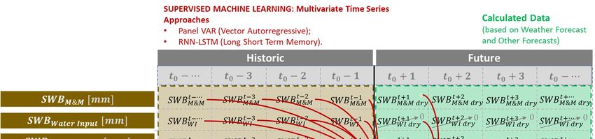
SWAMP - 777112                                                                                          03/05/2019

Disclaimer
This document contains material, which is the copyright of certain SWAMP contractors, and may not be
reproduced or copied without permission. All SWAMP consortium partners have agreed to the full
publication of this document. The commercial use of any information contained in this document may require
a license from the proprietor of that information. The SWAMP Consortium consists of the following

                                                                                     Part.
     Participant no.         Participant organisation name                           short         Country
                                                                                     name
     1 (European Coord.) Teknologian tutkimuskeskus VTT                              VTT               FI
     2                       Intercrop                                               ICRO              ES
     3                       University of Bologna                                   UBO               IT
     4                       Consorzio di Bonifica dell’Emilia Centrale              CBEC              IT
     5                       Quaternium                                              QUAT              ES
     6 (Brazilian Coord.)    Federal University of ABC                               ABC               BR
     7                       Centro Universitário da FEI                             FEI               BR
     8                       Federal University of Pernambuco                        UFPE              BR
     9                       LeverTech Tecnologia Sustentável                        LEV               BR
     10                      Brazilian Agricultural Research Corporation             EMBR              BR

companies:
The information in this document is provided “as is” and no guarantee or warranty is given that the
information is fit for any particular purpose. The user thereof uses the information at its sole risk and liability.

D3.1 Water Need Estimation                                                                                   2 of 43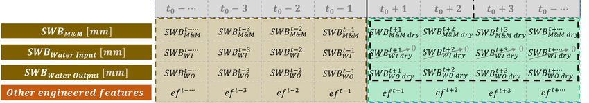
SWAMP - 777112                                                                                     03/05/2019

Document revision history
         Date          Issue      Author/Editor/Contributor           Summary of main changes
 21 January 2019       0.1     Attilio Toscano (UNIBO)        Preliminary document with standard
                                                              template layout.
 13 March 2019         0.2     Attilio Toscano, Camilla       First draft of the document
                               Stanghellini (UNIBO)
 22 March 2019         0.3     Juha-Pekka Soininen (VTT)      Additions to soil-based approach
 14 April 2019         0.4     Andre Torre Neto (Embrapa)     Addition of MATOPIBA pilot planned
                                                              application and validation of the
                                                              approaches
 18 April 2019         0.5     Andre Torre Neto (Embrapa)     Addition of Guaspari pilot planned
                                                              application and validation of the
                                                              approaches
 22 April 2019         0.6     Rodrigo Tognieri (ABC)         Revision of soil-based approach
 26 April 2019         0.7     Attilio Toscano, Camilla       Revision of the overall document
                               Stanghellini (UBO)
 03 May 2019           1.0     Juha-Pekka Soininen (VTT)      Changes to administrative data

Internal review history
             Date                          Reviewer                    Summary of comments
 29 April 2019                 Juha-Pekka Soininen (VTT)      Approved with comments
 29 April 2019                 Andre Torre Neto (Embrapa)     Approved with comments

D3.1 Water Need Estimation                                                                             3 of 43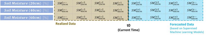
SWAMP - 777112                                                                                                                              03/05/2019

Table of contents
1     Executive Summary ............................................................................................................................ 5
2     Introduction........................................................................................................................................ 6
3     Modelling Water Needs ...................................................................................................................... 7
4     SWAMP approaches ..........................................................................................................................12
    4.1     Soil Measurement-Based Approach .............................................................................................12
      4.1.1      Approach Overview ...............................................................................................................12
      4.1.2      Feature Engineering ...............................................................................................................18
      4.1.3      Soil Moisture Forecast ...........................................................................................................19
      4.1.4      Soil Water Need Diagnosis ....................................................................................................21
      4.1.5      Soil Moisture Gap [%] to Soil Water Need [                              ] Conversion...............................................23
    4.2     Water balance based approach ...................................................................................................24
      4.2.1      CRITERIA: a model that integrates crop development and soil water balance .........................25
      4.2.2      Customization and improvement of CRITERIA within SWAMP ................................................30
5     Planned application and validation of the approaches ......................................................................36
    5.1     San Michele Fosdondo pilot (Italy) ...............................................................................................36
    5.2     Cartagena pilot (Spain) ................................................................................................................37
    5.3     MATOPIBA pilot (Brazil) ...............................................................................................................38
    5.4     Guaspari pilot (Brazil) ..................................................................................................................39
6     Summary ...........................................................................................................................................41
7     References .........................................................................................................................................42

D3.1 Water Need Estimation                                                                                                                        4 of 43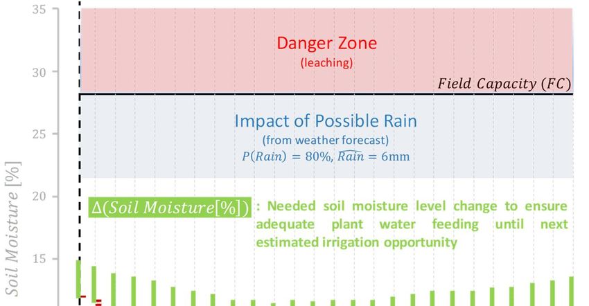
SWAMP - 777112                                                                                  03/05/2019

1 Executive Summary
This deliverable D3.1 Water Need Estimation results from Task 3.1. It summarizes the research carried out
concerning the estimation of irrigation needs, motivates the directions chosen for the project and presents
the approaches developed by the members of the SWAMP consortium.
Background concepts are briefly introduced in order to support the description of two specific modeling
approaches, that have been developed within the SWAMP activities. Those approaches are accurately
depicted both theoretically, in order to understand the mechanisms that drive them, and in an operational
way, with specific references to their application in the different pilot areas.

D3.1 Water Need Estimation                                                                          5 of 43
SWAMP - 777112                                                                                        03/05/2019

2 Introduction
The SWAMP project develops IoT based methods and approaches for smart water management in precision
irrigation domain and tests the approaches in four places, two pilots in Europe (Italy and Spain) and two pilots
in Brazil. The same underlying SWAMP platform can be customized into different SWAMP Systems according
to the needs of pilot deployments, considering different countries, climate, soil, and crops.

A key challenge in high precision irrigation scheduling, and consequently in the platform design, is the
knowledge of crop water requirements and within SWAMP it is addressed in Task 3.1 “Water need
estimation”. The task aims at defining the most suitable water requirements assessment strategies according
to the different pilot requirements. This document is the main output of Task 3.1 and presents the outcomes
of the research work performed during the first months of the project regarding the water need estimation
problem.

The examination of traditional models and of literature experiences led to the delineation of two approaches.
The first one, defined in the document as “Soil water content measurement-based approach”, basically relies
on the analysis with advanced analytical forecasting techniques of the data collected by soil moisture sensors.
The second one is called “Water balance based approach” because it exploits an existing analytic-empirical
model that is conveniently modified for the SWAMP purposes. The need of having two different approaches
comes from the differences that exist between the different pilots and that make some modelling aspects
more or less easy to implement. Enabling the platform to integrate different approaches make it more flexible
and capable of managing different real situations (small or large farms, flat or hilly areas, different irrigation
systems, organisation in management zones or not, etc.).

The document is organised as follows:

    1. Section 3 provides some general background concepts about the modelling of water exchanges in
       the soil-plant-atmosphere system and water needs, and it briefly presents some traditional models
       widely used. A lot of the terms introduced in this chapter will be further examined in the following
       sections.
    2. Section 4 accurately describes the two approaches developed within SWAMP, presenting their
       theoretical fundamentals and explaining how they will be implemented. Particular attention is
       devoted to show the use of the smart sensors within the models.
    3. Section 5 focuses more precisely on how each pilot will use one of the two approaches, with precise
       reference to the type of sensors used and their integration in the water estimation engine.

This deliverable is strongly related to deliverable D3.2 and in some way they are complementary: if D3.1
focuses on the water need according to the soil-plant conditions in order to avoid crop stress, D3.2 aims at
optimising the irrigation scheduling by taking into account other factors that might be influent (for example
costs and energy consumption). D3.1 is also closely related to D5.1: as the latter describes the specific
features of each pilot, it can be very useful to better understand how the water need assessment techniques
will be concretely deployed in each case study.

D3.1 Water Need Estimation                                                                                 6 of 43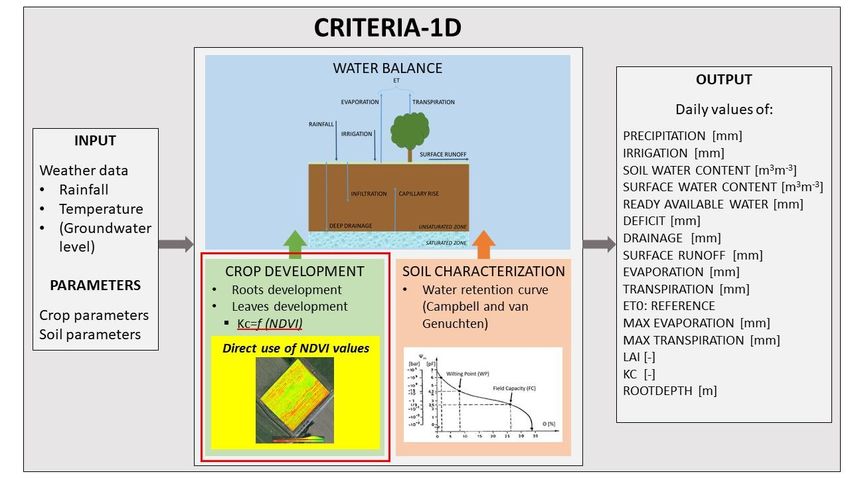
SWAMP - 777112                                                                                         03/05/2019

3 Modelling Water Needs
The starting point for the water needs assessment is the analysis of the water exchange process within the
soil-plant-atmosphere (SPA) system and of all the parameters that influence it. SPA is commonly
approximated to a single continuous system and the biophysical process of water motion trough it is called
transpiration. The transpiration process is driven by potential gradients and consists in the following stages:
a part of the water stored in the soil is absorbed by the roots, passes through the plant, enters part of it as a
constituent and finally reaches the leaves, where it evaporates and spreads into the atmosphere (Rallo 2010).
The amount of water that can be absorbed by the plant through the roots is governed by the potential
gradient in the soil. In fact, agricultural land does not contain water as a normal reservoir, but holds it against
gravity. At the same time, it forces the plant to spend energy to extract water from the ground. Each soil is
characterized by an empiric relation that links the water content to the water potential. The graphical
representation of this relationship is the water retention curve (Figure 1), whose shape depends on soil
texture and structure.

                             FIGURE 1 EXAMPLE OF WATER RETENTION CURVE FOR A MEDIUM TEXTURE SOIL

The soil water content Θ, or soil moisture, represents the ratio between the volume of water stored and the
total volume of soil, and it can be measured either in [m3m-3] or in [%]. The water potential ψm is defined as
the minimum work spent by the plant to extract the unit quantity of liquid from the soil. In the chart shown
by Figure 1 two significant values of water content can be identified (that can be seen in Figure 1) among
which the amount of water actually usable by the plant is included and that is called “available water”. The
wilting point (WP) is the minimum amount of water in the soil below which the plant is not able to extract
water anymore due to the high tensions: in this condition the water molecules are strongly held inside the
soil micropores. If the humidity falls below that value, the plant wilts and can no longer recover its turgidity.
The Field Capacity (FC) is the value of humidity that corresponds to the complete saturation of the
micropores. If that value is exceeded, the water can be no longer retained by the soil and it is then governed
by gravity that forces it to move downwards.
The two humidity values just defined delimit the amount of water retained in the root zone that is actually
available to the plants that is called total available water (TAW). Although water is theoretically available
until wilting point, as the water content of the soil decreases, so does the speed of absorption, leading the
plant to a stress condition. It is then necessary to define the readily available water (RAW) which represents
the fraction of the TAW that the plant is able to absorb without going into stress and changes according to
plant sensitivity to water shortage (Allen, et al. 1998).
In addition to monitoring the soil water content to detect when it drops below the threshold value, thus
causing stress to the plant, it is necessary to determine the amount of water released in the atmosphere in

D3.1 Water Need Estimation                                                                                  7 of 43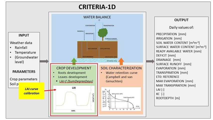
SWAMP - 777112                                                                                              03/05/2019

in the form of vapour during the final phase of the transpiration process. This value has been traditionally
identified as the crop water requirement: the reason is that almost the whole amount of water taken up from
the soil is lost by transpiration, while a little fraction of it is used within the plant (Allen, et al. 1998). The well-
known “FAO Irrigation and Drainage Paper No. 56” defines the crop water requirement as the amount of
water needed to balance the evapotranspiration, and consequently the irrigation water requirement as the
difference between the crop water requirement and effective precipitation (Allen, et al. 1998). It can be
noticed that the term used to describe the process in this case is evapotranspiration, defined as the
combination of transpiration from plants and evaporation from soil. The need to group the two comes from
the fact that it is difficult to tell apart the two contributions as they take place concurrently, and also from
the consideration that both types of loss must be taken into account for the water balance assessment.
As it is hard to perform direct measurements of the evapotranspiration rate, the possibility to assess this
variable with models has long been studied: a universally accepted collection of guidelines for this purpose
can be found in the above mentioned Paper No. 56 by FAO. In the document it is explained that the
evapotranspiration process is influenced by weather parameters, crop characteristics, management and
environmental aspects. Therefore, all of these aspects should be considered when modelling it. The FAO
approach takes them into account by introducing different terms, each one related to one of them (Allen, et
al. 1998).
The reference evapotranspiration ET0 is used to quantify the evapotranspiration potential of a given area. In
fact, it is calculated for a reference crop (festuca arundinacea, Schreb., Multispecies grass) under ideal
conditions (uniform coverage, ample water availability). ET0 is only affected by climatic parameters, not by
soil and crop characteristics, so it allows the characterization of a given area independently from the crops
grown and the agronomic techniques used. Thus, ET0 is considered a climatic parameter as well and it can be
computed from weather data with different models. Among them, the FAO Penman-Monteith is particularly
convenient because it closely approximates grass ET0 at the evaluated location, it is physically based, and it
explicitly incorporates both physiological and aerodynamic parameters (Allen, et al. 1998). The origin is the
1948 Penman model that computed evaporation from an open water surface from standard climatological
records of sunshine, temperature, humidity and wind speed. This early version has been modified several
times in order to extend it to cropped surfaces by introducing resistance factors. The FAO Penman-Monteith
version of it was established by FAO as the reference model for ET 0 estimation and can be written as follows:
                                                                 900
                                         0,408 (    − )+
                                     =                           + 273 (         −     )
                                                     ∆+     (1 + 0,34 )

where:
    •    ET0 reference evapotranspiration [mm day-1];
    •    Rn net radiation at the crop surface [MJ m-2 day-1];
    •    G soil heat flux density [MJ m-2 day-1];
    •    T mean daily air temperature at 2 m height [°C];
    •    u2 wind speed at 2 m height [m s-1];
    •    es saturation vapour pressure [kPa];
    •    ea actual vapour pressure [kPa];
    •    es-ea saturation vapour pressure deficit [kPa];
    •    Δ slope vapour pressure curve [kPa °C-1]
    •    γ psychrometric constant [kPa °C-1].

To study how the process changes according to the peculiarities of the crop and its growing stage, the
evapotranspiration under standard conditions (ETC) is defined. This variable refers to evapotranspiration
from disease-free, well-watered and well-fertilized crops, under optimum conditions of soil and resulting in
full production. The most common approach consists in determining ETC by multiplying ET0 for a crop

D3.1 Water Need Estimation                                                                                       8 of 43
SWAMP - 777112                                                                                               03/05/2019

coefficient (Kc) that integrates and summarizes the characteristics that differentiate the cropped surface
from the reference surface.
                                                         =
Kc varies mainly with the specific crop characteristics and is only marginally influenced by climate, so that the
same standard values for Kc can be used for different locations and climates. For this reason, the Kc-approach
has been widely accepted and used.
The deviation from standards of management and environmental conditions has an effect on the
evapotranspiration, so that ETC must be suitably corrected. The FAO approach suggests addressing it
adjusting the Kc values to field conditions and introducing stress coefficients (Allen, et al. 1998) (Figure 2).

           FIGURE 2 REFERENCE (ETO), CROP EVAPOTRANSPIRATION UNDER STANDARD (ETC) AND NON-STANDARD CONDITIONS (ETC ADJ)
                                                         (ALLEN, ET AL. 1998)

It is evident that the irrigation scheduling in terms of amount and timing is particularly complex considering
the large number of aspects that influence irrigation: soil and crop properties, features of the irrigation
system, and environmental factors. To simplify the work of farmers and to overcome the traditional approach
based on experience, several decision support tools have been developed over the years. The mathematical
models can be either physically based or empirical: the first category includes those that are based on the
equations of mass and energy conservation, the second consists in relationships between the variables that
are retrieved from the experience. Simulation models can be useful for different purposes. Firstly, they can
be used to estimate a large number of variables that characterize the SPA (Soil-Plant-Atmosphere) system
without having to measure all of them: they can be determined starting from the model equations and can

D3.1 Water Need Estimation                                                                                        9 of 43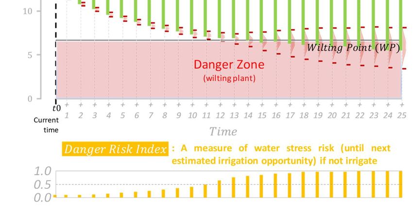
SWAMP - 777112                                                                                          03/05/2019

be used to direct possible field test in a more time and cost effective way. Another application, as already
mentioned, is to use them as decision support tools for SPA system management.
An example is Aquacrop, a simulation model developed by the Land and Water Division of FAO that simulates
the SPA system modelling (Steduto, et al. 2009):
    •   the soil, with its water balance;
    •   the plant, with its growth, development, and yield processes;
    •   the atmosphere, with its thermal regime, rainfall, evaporative demand, and carbon dioxide
        concentration;
    •   some management aspects, with emphasis on irrigation (Steduto, et al. 2009).

In the figure below (Figure 3) a general scheme of Aquacrop.

FIGURE 3 CHART OF AQUACROP INDICATING THE MAIN COMPONENTS OF THE SOIL–PLANT–ATMOSPHERE CONTINUUM AND THE PARAMETERS
         DRIVING PHENOLOGY, CANOPY COVER, TRANSPIRATION, BIOMASS PRODUCTION, AND FINAL YIELD (STEDUTO, ET AL. 2009)

Aquacrop is a canopy-level model that mainly focuses on the assessment of attainable crop biomass and
harvestable yield in response to water, considered as a key driver of agricultural production (Figure 3). The
irrigation option can be “rainfed” (no irrigation) or it can be set defining the application method (sprinkler,
drip, or surface) and the schedule by specifying the time and depth of each application. The setting can be
done either by the user or automatically by the program. This approach relies on the agronomic experience
of the user that sets the parameters, but is not oriented to optimization (Steduto, et al. 2009). Even if
Aquacrop code is not freely available, several studies tried to improve this aspect using the software as a
black box and including it into an optimization algorithm in order to get the optimal irrigation scheduling
(Ioslovich and Linker 2015) (Pham , Saleem and Okello 2013).
A similar approach to irrigation management is followed by CROPWAT, a computer program as well
developed by the Land and Water Division of FAO that can be used for the calculation of crop water
requirements and irrigation requirements based on soil, climate and crop data (Smith 1992).

D3.1 Water Need Estimation                                                                                 10 of 43
SWAMP - 777112 03/05/2019 Another model that shares some of the Aquacrop features is Criteria-1D that will be accurately described in the chapter 4.2.1. D3.1 Water Need Estimation 11 of 43
SWAMP - 777112 03/05/2019
4 SWAMP approaches
To plan an effective irrigation scheduling it is essential to know the amount of water in soil available to the
crop as well as the evapotranspiration rate of the vegetation. SWAMP will handle this task integrating the
modelling of the physical system with smart sensors’ data. Two different approaches are developed:
1. Approach #1: based on the modelling of the storage capacity of the soil and the integration of soil
moisture measurements;
2. Approach #2: aims at integrating multispectral data gathered from drones in an existing simulation
model to calculate the water balance according to the observed vegetation growth.
4.1 Soil Measurement-Based Approach
The development of IoT has made possible the acquisition of more abundant, reliable and low-cost data
(Whitmore and Agarwal 2015). Furthermore, the advance of data analytical techniques and availability of
computational power enable the use of water need estimation methods based directly on soil water content
measurements rather than ad-hoc physical soil models.
Thinking more specifically about the problem of water needs at its present stage, we can observe that it is
easier to obtain information about some phenomena than from others. For examples, soil water content can
be directly measured, while evapotranspiration cannot (it will be detailed below). And this can help in
deciding whether our approach should be based exclusively on analytical data and techniques, or whether
we should allow the use of physical models.
For example, soil moisture sensors bring the main variable of interest when it comes to irrigation, which is
the soil water content, and, in addition, their continuous data bring implicit information of the soil water
dynamics. Therefore, using the soil data directly in an analytical technique might be a profitable investment.
A counter example is evapotranspiration, which is another important element for irrigation need evaluation
corresponding to the meteorological variables. This variable cannot be measured directly in an easy way,
being usually calculated by physical models. Such a difficulty in a more direct measurement leads us to
conclude that, with respect to evapotranspiration, a more prudent approach might be to use physical models
to intermediate data and analytical techniques.
Therefore, when it comes to the soil measurement-based approach, the SWAMP project will focus on a
hybrid approach, which favors a more direct reading of data and the use of new advanced analytical
techniques, but still seeks to take advantage of physical models as input. Our key assumption is the
hypothesis that the physical models facilitate the work of analytical techniques to absorb nonlinearities,
irregularities and to identify and clean data noise.
The main idea of this approach is to create the detailed volumetric water content forecasts for the crop’s
root area by applying advanced analytical forecasting techniques on soil water content data (soil moisture),
and on Soil Water Balance data. Water balance data is composed of direct measurement stimuli (occurrence
of rainfall and irrigation), and indirect measurement stimuli (such as the effects of evapotranspiration, deep
percolation, capillary rise and runoff).
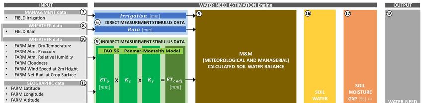
Figure 4 summarizes this approach, already specifying the data, processes and techniques that we intend to
use. The Input column specifies the data that will be used as base of information, and they are there
organized and classified according to their origin nature. The Water Need Estimation Engine column specifies
the processes flow and all processes themselves by which the data will pass. Finally, the Output column
D3.1 Water Need Estimation 12 of 43SWAMP - 777112 03/05/2019
specifies the intended approach outcome, which is the Water Need Estimation at the present time and in the
future, accompanied by critical-level risk measurements.
FIGURE 4: SOIL MEASUREMENT-BASED APPROACH OVERVIEW
Next, in this section, the main elements of Figure 4 are detailed.
Soil Moisture Forecast process can be identified in Figure 4 by label 1. This process is the most central of the
Water Need Estimation engine because all previous processes on the flow converge to it. In addition, it
represents directly the main idea of this approach, that is, the direct operation of advanced analytical
forecasting techniques on:
• The soil water content data (soil moisture);
• Plus the soil water balance data, which, in turn, is composed of:
o Direct measurement stimuli data (occurrence of rainfall and irrigation), and of
o Indirect measurement stimuli data (such as the effects of , deep percolation, capillary rise
and runoff, calculated from physical models – preferably those free of regionalisms).
For this case, multivariate forecast techniques are applicable:
a) Panel VAR (Vector Autorregressive) (Canova and Ciccarelli 2013): a traditional multivariate time
series forecast technique, which can also be used if eventual qualitative predictors are needed.
Technically, it is a stochastic model designed to capture linear interdependence among multiple time
series. It is a generalization of autoregressive model to time series regressions, where the lagged
values of all series appears as regressors. In other words, we regress a vector of time series
variables on lagged vectors of these variables. VAR has been used to calculate evapotranspiration in
(Nugroho, Hartati and Mustofa 2014); and
b) RNN-LSTM (Recurrent Neural Network, using Long Short-Term Memory architecture) (Goodfellow,
Bengio and Courville 2015): RNN is a technique of the Deep Neural Networks field that when used
under the LSTM architecture usually obtains high performance in multivariate time series
applications. In recurrent neural networks, connections between nodes form a directed graph along
a sequence. This characteristic makes such networks suitable for sequential and time series data.
LSTM is a special kind recurrent neural networks capable of learning long term dependencies. It does
D3.1 Water Need Estimation 13 of 43SWAMP - 777112 03/05/2019
this by introducing a memory unit (called cell), which can modulate the output based on the internal
cell state. It was used in (Adeyemi, et al. 2018) for soil moisture content prediction for irrigation
scheduling.
We aim to test both techniques listed: the more traditional Panel VAR and the more modern RNN-LSTM.
Obviously, we believe on a higher performance of RNN-LSTM assuming that Deep Neural Networks have
been able to better absorb nonlinearities, irregularities and noise in recent time series applications (Liu, et
al. 2017), although it is not easy to adjust the artificial neural network architecture for specific applications.
The VAR Panel, besides being a suitable benchmark (Canova and Ciccarelli 2013), is the safe choice because
its performance in multivariate time series is already traditionally appropriate and there is no need for
architecture adjustments as in the case of RNN-LSTM.
Ideally, the forecast will be performed on an hourly time step with a forecast horizon of a few hours or days,
depending on the periodicity of the input data provided. If the data are made available on an hourly or intra-
hourly basis, the forecast will have an hourly time step. If the data are available at a frequency greater than
the hour, the forecast will be daily.
The data structure for the above-mentioned techniques, as well as more details of the techniques themselves
and how they will be applied will be given in section 4.1.3.
Soil Water Content Data can be identified in Figure 4 by label 2. The main input of the Soil Moisture Forecast
process is soil water content data (measured as soil moisture), as these are basically the direct
representatives of the variable we want to predict (soil moisture). Soil Water Content Data is composed of
Soil Sensors Data and complemented by Soil Characterization Data.
Soil Sensors Data can be identified in Figure 4 by label 3. For each location on the farm where a soil sensor
module is installed, the soil moisture measurements are collected periodically at different depths.
Measurement at different depths is important for two reasons:
• Firstly, because the plant root extracts water from the soil for the entire depth of its extension. At
early stages of the plant development, the root is short, but over time, it reaches greater depths, so
that the importance of each depth is variable in time (Bittelli, Campbell and Tomei 2015).
• Secondly, because soil dynamics is potentially different in different depths due to different degrees
of compaction and density (implying distinct retention, percolation and capillary effects), and also
due to influences of upper and lower depth behavior, as well as other variables (soil slope, for
example) (Bittelli, Campbell and Tomei 2015) 1.
Preferably, at least one soil sensor module per management zone (field) must be installed. And given the
possibility of ideally working with an hourly forecast time step over a forecast horizon of a few hours or days,
it might also be interesting if the data were collected minimally in hourly samples.
Soil Characterization Data can be identified in Figure 4 by label 4. Soil characteristics for water retention
should be considered as complement to pure soil sensor data as a way of mapping the sensor data use.
It is a way of adding to the analytical techniques (of the Soil Moisture Forecast process) valuable information
mainly of nonlinearities and discontinuities regarding soil water retention, difficult to be absorbed by the
analytical techniques. Thus, it may be said, it is a way of facilitating the work of the analytical techniques.
The main references of water retention curve modeling are Campbell and Van Genuchten (Bittelli, Campbell
and Tomei 2015), and these are the candidates to be used to obtain the specific curves for each management
zone (field) and depth. The process to obtain this curve is empirical and done before the crop cycle begins.
1
That is, there are a number of nonlinearities, time lags and irregularities to be captured for a Soil Moisture Forecast process to succeed.
D3.1 Water Need Estimation 14 of 43SWAMP - 777112 03/05/2019
Calculated Soil Water Balance process can be identified in Figure 4 by label 5. Soil water balance information
is desirable for Soil Moisture Forecast process techniques as it complements the information of soil water
content with information on the relative water level variation stimuli in the analyzed system.
Basically, these stimuli are inputs or outputs of water in the system (Allen, et al. 1998) (Bittelli, Campbell and
Tomei 2015). Occurrences of rainfall and irrigation, as well as capillary rise, are inputs of water into the
system. Evapotranspiration and deep percolation are examples of system water outputs. Exchanges with
other soil depths and runoff are examples of input or output depending on direction and orientation.
In this approach the soil water balance and its components are only considering the managerial (irrigation)
and meteorological influences (rain and evapotranspiration) 2, leaving aside mainly the influences of the soil
dynamics (deep percolation, capillary rise and runoff). Soil dynamics influences are not being considered in
the physical models gap because they are supposed to being implicitly captured by the soil moisture data
processed by analytical techniques (Soil Moisture Forecast process).
At this stage, the idea is to compute the managerial and meteorological (M&M) balance of transient water
in each period, resulting in the M&M Calculated Soil Water Balance ( & ) and its components
( and ), as in the equations below. They may be predictive variables in the
Soil Moisture Forecast process.
& = + − [ ]
= + [ ]
=− [ ]
The inputs to the & Calculated Soil Water Balance can be divided into direct measurement stimuli data
and indirect measurement stimuli data, both detailed below.
Direct Measurement Stimuli Data can be identified in Figure 4 by label 6. Direct measurement stimuli are
those that can be measured without much difficulty in a direct way, without the use of models. In our case,
both irrigation management events (Figure 4 - label 7) and rainfall events (Figure 4 - label 8) can be measured
directly.
Indirect Measurement Stimuli Data can be identified in Figure 4 by label 9. Indirect measurement stimuli are
those measured through models because of the high difficulty or impossibility of direct measurement. It is
on this occasion that the physical models can be used in our hybrid approach, for the possibility of estimating
important values that could not otherwise be disposed (or at least not easily), by incorporating irregularities
and non-linearities among the component variables, and also due to the high independence level of the
model in relation to noise (the influence of noise is stronger on direct measurement variables).
Within the context of precision irrigation, useful physical models calculate adjusted crop evapotranspiration,
soil water dynamics (deep percolation, capillary rise and runoff) and the plants growing stage. Given that
SWAMP seeks to build a platform that can be used in pilots in different countries, with different conditions,
another interesting characteristic of physical models is that they are not only valid for limited regions or for
certain meteorological conditions, but also can be as comprehensive as possible.
For the physical models gap, we decided to use the Penman-Monteith (FAO 56) (Allen, et al. 1998) model,
which calculates adjusted crop evapotranspiration, whereas soil dynamics will be based on direct soil
measurements. The reasons for choosing this configuration were two:
a) The Penman-Monteith model is considered the most complete and comprehensive
evapotranspiration model, and has been tested and confirmed as such for almost 20 years;
2
Therefore taking the name & , where & stands for Managerial and Meteorological.
D3.1 Water Need Estimation 15 of 43SWAMP - 777112 03/05/2019
b) We prefer to use hourly time step in forecasting the water need so that an irrigation optimization
approach may have the opportunity to choose the best time of day for irrigation. In this context, the
Penman-Monteith model is one of the few that has an hourly version.
The input data for the Penman-Monteith model are meteorological (Figure 4 - label 10), geographical (Figure
4 - label 11), temporal (Figure 4 - label 12) and of crop development (Figure 4 - labels 13 and 14). For the
latter, essential for the calculation of the evapotranspiration crop coefficient ( ), the ideal would be to use
LAI (Leaf Area Index) or NDVI (Normalized Difference Vegetation Index) (Carlson and Ripley 1997) as ideal
setting. These parameters can be evaluated by multispectral images while, if drones or satellites cannot be
used, the determining factors for crop development will be plants height and density, and the measurements
will be made manually and periodically (Allen, et al. 1998).
Feature Engineering process can be identified in Figure 4 by the label 15. Feature engineering is the work
that makes use of domain knowledge and KDD (Knowledge-Discovery in Databases) techniques to create new
features (variables) that make the analytical techniques achieve superior results, because they capture non-
explicit and non-trivial extractable behaviors in the data (Chandrashekar and Sahin 2014). In our case, it is
the process immediately preceding the Soil Moisture Forecast process. Its function is to construct new
features (variables) from previously generated input variables, which may facilitate the work of Soil Moisture
Forecast process analytical techniques.
The main types of new variables that are usually extracted by this procedure are (Chandrashekar and Sahin
2014): a) temporal lag values, so that analytical techniques can capture delayed effects of one variable into
another; b) non-linearities between two or more variables, so that the analytical techniques can correctly
consider the sensitivity in change of variable values; c) combination of variables, so that analytical techniques
can capture more directly the interaction of closely dependent variables; d) decomposition of variables, so
that analytical techniques can consider as separate signs the seasonal effects and other locally and
momentarily significant effects; e) categorization of metric variables, which may be more appropriate to
some analytical techniques; f) dimensional reduction and variables orthogonalization, so that analytical
techniques have a simpler and more organized information scenario from the input data.
Two approaches will be tested for the development of new feature variables (Chandrashekar and Sahin
2014): I) Manual Feature Engineering: Agronomists, farmers and data scientists will use their tacit application
domain knowledge and the data to suggest the new variables; II) Automated Feature Engineering: KDD
techniques will be used to suggest variables discovered automatically.
More details about the techniques used in feature engineering will be given in section 4.1.2.
Soil Water Need Diagnosis process can be identified in Figure 4 by label 16. The Soil Moisture Forecast
process outputs the predicted soil water content (soil moisture) for each of the soil depths along the chosen
forecast horizon (which is intended to be at least two days) with forecast points in the chosen timestep (which
is intended to be hourly, or at least daily). In addition to the estimated values, each point along the forecast
horizon is provided of the information on the uncertainty distributions.
This output is in turn the input to the Soil Water Need Diagnosis process, which combines it with the
information of root development (Crop Development Data) and rain data (Weather Data) to output
measurements of:
a) What would be the needed soil water content gap (soil moisture), represented by
∆( [%]);
b) What is the criticality of this need at each timestep point to avoid water stress / wilting point levels,
represented by the [%].
The water need gap calculation should not only consider the water need in its reference time, but also
consider the temporal lag effect on soil moisture after the water supply. This is because, depending on the
depth of the soil and its retention characteristics, the effects are felt with time lags and smoothed over time.
D3.1 Water Need Estimation 16 of 43SWAMP - 777112 03/05/2019
In addition, it is necessary to consider each depth in a weighted way according to the distribution of the rooting
system.
Such measures are of great importance to answer the fundamental questions of water need estimation: how
much water is and will be needed, and what is the criticality of making the supply in each time step of the
forecast horizon?
This process is better detailed in a separate section 4.1.4.
Soil Moisture Gap [%] to Soil Water Need [mm] Conversion process can be identified in Figure 4 by label 17.
Among the Soil Water Need Diagnosis process outputs, the needed soil water content gap has the
inconvenience that it cannot be used directly by the Irrigation Optimization approach 3. This is because soil
moisture, and hence the soil moisture gap, is traditionally measured as % of the maximum water capacity in
the soil, whereas an irrigation optimizer would need to receive a more direct indication of what water blade
(soil water need) would be required, measured in .
Thus, it is necessary to have a process of converting soil moisture gap [%] into soil water need [ ], and
this is exactly what the present process proposes to do. Iconographically, we have:
∆( [%]) → ∆( [ ])
With:
∆( [ ]) = ( [%], ∆( [%]))
A more detailed description of this process is given in section 4.1.5.
Water Need Estimate the final output of this approach, can be identified in Figure 4 by label 18. It is obtained
from the joint actuation of Soil Water Need Diagnosis process and Soil Moisture Gap [%] to Soil Water Need
[mm] Conversion process, and consists of two components:
a) The needed soil water content gap (water blade, measured in [ ]), represented by
∆( [ ]); and
b) The criticality of this need at each timestep point to avoid water stress / wilting point levels,
represented by the [%].
The two measurements above, geolocated for each of the management zones (fields) or even for each soil
sensor module, will be inputs to the Irrigation Optimization approach (deliverable D3.2 of the SWAMP
Project) to decide when is the best moment to irrigate and how much water to manage considering all the
operational restrictions. Figure 5: ILLUSTRATION OF WATER NEED ESTIMATION OUTPUTS below illustrates
the two measurements as outputs, where it is possible to visualize ∆( [ ]) and
[%] for each hourly time step in the forecast horizon.
3
Described in another SWAMP project document, the deliverable 3.2 (D3.2).
D3.1 Water Need Estimation 17 of 43SWAMP - 777112 03/05/2019
∆( ) : Needed water blade supply to ensure
adequate plant water feeding until next
estimated irrigation opportunity
10
5
0
: A measure of water stress risk (until next
estimated irrigation opportunity) if not irrigate
1.0
0.5
0.0
0+ + + + + + + + + + + + + + + + + + + + + + + + +
Current
1 2 3 4 5 6 7 8 9 10 11 12 13 14 15 16 17 18 19 20 21 22 23 24 25
time
FIGURE 5: ILLUSTRATION OF WATER NEED ESTIMATION OUTPUTS
Differently from mathematical based soil models, which rely on domain expert knowledge about soil types
to calculate soil properties, measurement-based approach can make use of potentially more accurate
proximal soil sensing. On the other hand, in order to prepare data for modeling the soil-crop-atmosphere
water balance, there is a need of data processing methods for dealing with measurement errors, large
volume and variability of data, and feature engineering techniques for preparing data in a suitable way for
applying analytical techniques.
Here are the feature engineering techniques that can be used in this approach and how:
a) Upsampling/Downsampling: sometimes the time series data are given in different time scales. In
these cases, it may be necessary to do some kind of resampling to adjust the time scales. In
upsampling, we increase the frequency of the frequency of the samples. To this end, some
interpolation method is used to fill in the missing samples in the new frequency. In downsampling,
we decrease the sample frequency of the series. To do this, we can use a pooling function, described
next.
b) Min/Max/Average/interquartiles/Sum pooling: Pooling functions take as input a (slice of a) time
series and return their minimum, maximum, average, interquartile ranges or sum.
c) Rolling window statistics: Rolling window statistics correspond to the application of some pooling
function over a sliding window in the time series. To do this, a fixed feature derivation window similar
to lagged features is used as input to a pooling function.
d) Expanding window statistics: Expanding window statistics are similar to rolling window statistics, but
it is computed considering a window containing all points from the beginning of the series until the
forecast point.
e) Data transformation: some techniques require data transformation before feeding it to an algorithm.
This transformation may include, for instance, box-cox transformation to stabilize variance or z-
scores transformation to adjust for scale (Sakia 1992).
f) Covariates calculation: soil properties can be measured at different levels, or more than one probe
can be used in some farms. For some techniques, it will be interesting to incorporate depth or spatial
covariates. These covariates can be used, for instance, in Panel VAR (Vector Autorregressive)
algorithms.
D3.1 Water Need Estimation 18 of 43SWAMP - 777112 03/05/2019
g) LSTM (Long Short-Term Memory) Autoencoders: Recently, neural networks are being used to
automatically extract features from data. The main idea is to use a neural network to “predict” as
output the same data used as input (self-supervision). With the aid of layers with smaller dimensions
than the input data, the network can be trained to learn a lower dimensional embedding space,
removing covariates and filtering out noise. These networks are called autoencoders, which can be
used to learn compressed representation of sequence data and have been used on video, text, audio,
and time series sequence data. In the case of time series sequence data, a popular approach is the
LSTM autoencoders, as LSTM networks are widely used for time series forecasting.
h) Feature combination: in some cases, we can to combine some features to better explore their
relationship. For instance, depending on the crop stage, it may be interesting to combine the soil
water content at different depths. In earlier stages of the crop development, for instance, when the
roots are closer to the soil surface, the two deepest depths could be combined to better represent
the water content not in the root zone.
Conceptually, the soil moisture forecast process could be seen as multivariate time series forecast, where
data from soil sensors, past weather information and weather forecasts, as well as crop development status
are used to infer a likely range of soil moisture for a near future time frame.
This prediction can then be used for irrigation decision-making (as described in SWAMP deliverables D3.2
and D3.3). To accomplish this, considering the instant as the forecast point, we use data from a time window
ranging from [ − ∆ , … , ] as input, aiming at predicting the soil moisture in a future time window [ +
1, … , + ∆ ] where ∆ and ∆ are user defined parameters.
Based on this historic and future time windows, we can use the lagging feature extraction technique (Section
4.1.2) applied to multivariate time series, and transform it to a supervised machine learning problem as
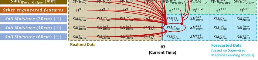
shown in Figure 6: SOIL MOISTURE FORECAST PROCESS DATA STRUCTURE – PART 1. The multiple time series
considered are the soil moistures measured at different depths (the figure represents three different depths
- 20, 40 and 60 ), as well as Soil Water Balance ( & ) and its components ( and
). Upsampling or Downsampling (Section 4.1.2) may be necessary to adjust for different
time resolutions.
FIGURE 6: SOIL MOISTURE FORECAST PROCESS DATA STRUCTURE – PART 1
Past weather information and weather forecasts can be incorporated either as raw values, or by considering
their rolling window statistics (hourly measured air temperature, for instance, can be transformed to a daily
air temperature amplitude).
D3.1 Water Need Estimation 19 of 43SWAMP - 777112 03/05/2019
In our hybrid framework, as illustrated in Figure 7: SOIL MOISTURE FORECAST PROCESS DATA STRUCTURE –
PART 2, we intend to use estimated future evapotranspiration to calculate Soil Water Balance
( & ) and its components ( and ). The reason is that, by doing this, we
can have a good estimation of , i.e., at driest condition (no rain and no irrigation).
FIGURE 7: SOIL MOISTURE FORECAST PROCESS DATA STRUCTURE – PART 2
The past historical data, augmented with (green box in Figure 7), can then be feed to multivariate
forecast algorithms to predict the values of . The process can be repeated to all [ + 1, … , + ∆ ],
as shown in Figure 8.
FIGURE 8: SOIL MOISTURE FORECAST PROCESS DATA STRUCTURE – PART 3 (TECHNIQUE APPLICATION)
The two analytical techniques (Panel VAR and RNN-LSTM) we plan to use for multivariate time-series
modelling are stated and explained in Section 4.1.1.
D3.1 Water Need Estimation 20 of 43SWAMP - 777112 03/05/2019
Basically, this process receives as inputs:
a) Soil moisture forecast model, so that it can be used in simulations of future scenarios (origin: Soil
Moisture Forecast process);
b) "Dry" soil moisture forecast, considering the worst case in the future - where = 0 and
= 0 -, with all future soil moisture points (* with their respective error probability
distributions) of timestep time within the forecast horizon (origin: Soil Moisture Forecast process);
c) Rain forecasted amount and probability for the next period, so that the water need estimation can
avoids leaching risk in case of expected rainfall (origin: Weather Data);
d) Roots development information, so that it is possible to know the soil depths importance proportion
by the distribution of root sucking area (origin: Crop Development Data).
As outputs, this process produces:
a) Soil water content gap, represented by the ∆( [%]) metric: in other words, this metric
answers the following question. If the next irrigation had occurred at a specific current or future time,
what would been the soil moisture variation that would allow the soil to maintain safe soil water
content levels until the next estimated irrigation opportunity. The exact number is calculated using
simulation and the soil moisture forecast model, also considering predicted values of meteorological
variables, to verify, if the water amount is enough for the estimated next opportunity for irrigation.
Figure 9 illustrates this quantity calculation in two distinct moments, (A) 0 and (B) + 12 (just for
exemplification purposes, but this procedure is performed for every point of the hourly time step).
The red distribution series over the forecast horizon represents the worst (driest) forecasted
condition, and the blue is the one that would have occurred, if irrigation was done with its ideal soil
moisture gap (∆( [%], green bar) for that irrigation opportunity. An ideal soil moisture
gap is the one that is minimum, and also guarantees that water level will not be in the wilting point
danger zone before the estimated next opportunity for irrigation. The impact of possible rain
information is there to make the algorithm avoid deciding for a soil moisture delta to risk reaching
the leaching danger zone;
D3.1 Water Need Estimation 21 of 43SWAMP - 777112 03/05/2019
FIGURE 9: EXAMPLES OF CALCULUS OF ∆( [%]) FOR TWO DIFFERENT TIMES, E +
b) : representing what is the criticality of this water need at each time step in order
to avoid water stress or wilting point levels. Index is calculated for all time points until next estimated
irrigation opportunity aggregating (by average) the probabilities of the soil water content level being
below the Wilting Point of all the future time points, i.e., considering the proportion of red probability
distributions of future points that are below Wilting Point line.
Figure 10 highlights these cited metrics, calculated in the forecast horizon and chosen time step (hourly)
context, always acting on the base scenario, the dry forecast. It is the generalization of Figure 9, with all the
ideal soil moisture gaps (∆( [%], green bars), one for each time step point. It also brings the
(yellow bars) for each respective point.
D3.1 Water Need Estimation 22 of 43SWAMP - 777112 03/05/2019
FIGURE 10: ILLUSTRATION OF SOIL WATER NEED DIAGNOSIS, WITH ITS TWO METRICS WITH POINTS THROUGH THE TIME STEP OF THE
FORECAST HORIZON: ∆( [%]) AND
The output of Figure 10 are produced for each soil depth. Then it is necessary to add the use of Root
Development Data, so that, when knowing the relevance of each depth, we can calculate single weighted
values of ∆( [%]) and , for each management zone (field) or even soil
sensor module.
Sensors Contextualization
Proper timing and depth of irrigation can contribute to increase crop yield and decrease nutrient and soil
losses. Both factors can be accurately achieved using soil moisture sensors. Moreover, water use efficiency
can be substantially improved by coupling variable rate irrigation (VRI) technology with soil moisture sensor
networks and dynamic irrigation scheduling tools. Those are the premises of the proposed approach of
controlling irrigation by soil moisture conditions.
The two mostly indicated soil moisture sensors for agricultural usage are the capacitance sensors that
measure the volumetric water content ( ), and the tensiometric sensors that measure soil matric
potential or soil water tension ( ). is exactly what the name suggests, i.e., the volume of water
contained in a certain volume of soil and it is simply expressed by a percentage or a fraction of unit in cubic
volume by cubic volume (e.g. ∙ ). is the amount of energy required by plants to extract water
from soil and it is measured in units of kilo Pascals ( ) or centibars ( ). There are accepted values of
for wilting point and field capacity and those values do not depend on soil type. On the other hand, these
benchmark conditions cannot be directly expressed by due to its dependence on soil type. An ideal
soil-based irrigation method would make use of both sensors, data ( ) to provide the critical values
and data ( ∙ ) to calculate the volume of water needed to reestablish a desired soil moisture
condition (field capacity or a fraction of it).
D3.1 Water Need Estimation 23 of 43SWAMP - 777112 03/05/2019
The SWAMP Soil Measurement-Based approach irrigation control will make use of capacitance sensor to
measure water in soil. Critical soil moisture values can be obtained by two methods: a) calculated from
data and soil specific retention curve or b) from allowable soil water ( ) depletion values. or
depletion critical values shall be found in the literature or obtained in laboratory. The water need volume
will be calculated straight from the data for both cases.
Soil Moisture Gap to Soil Water Need
As seen in 4.1.1, the Soil Moisture Gap measure must be converted to mm, being renamed to Soil Water
Need, in order to be used by the irrigation system. This section aims to show how to do this conversion as
follows.
The proper calculation of water storage ( ) in any soil profile from depth to depth is as follows:
= ( )∙
where [ ∙ ] is the volumetric water content along the soil water content profile, considering
the depth dimension.
The soil probe measures at specific depths and not along the profile. Therefore, it is assumed the same
value of the volumetric water content along the soil profile section that the sensor element at a certain depth
is representing. The water storage of that section of length turns to be:
= ∙
The necessary irrigation volume in length by unit area ( ) to replenish the soil section to the ideal level is
similarly calculated by:
= ( − )∙
The equations above follow the sensors traditional iconography. However, to make them make sense in this
text, we should rewrite the last equation with the notation used in this document, making =
∆( [ ]) and = [%]. Then:
∆( [ ]) = ( [%] − [%] )∙
Simplifying:
∆( [ ]) = ∆( [%]) ∙
4.2 Water balance based approach
Crop water requirements can be determined by assessing the various components of the soil water balance,
i.e. considering the incoming and outgoing water flux into the crop root zone over some time period. As seen
in 3.1, several models are available for such computation. The one chosen for SWAMP is CRITERIA-1D, a
simulation model of the hydrological balance of the agricultural field that describes the development of the
plant.
CRITERIA-1D works on a daily scale and overlooks spatial variability, assuming that the field is all concentrated
in one point and that the water exchanges taken into consideration are those that occur in the vertical
direction. This assumption is consistent if the soil characteristics are homogeneous across the studied field
(so that one point can be assumed to be representative of the whole field) and if the location is a flat area
where the water movement in horizontal direction is negligible. That is for example applicable to the Po plain
area in Italy, where the farms have medium-small size and are located in a zone where no significant slopes
are present.
The model was developed by Arpae-Simc over the years and was chosen for SWAMP due to some key factors.
First of all, CRITERIA-1D has the remarkable advantage of being open source and of making its code available
under the LGPL license, thus allowing any software modifications. Furthermore, the collaboration with some
D3.1 Water Need Estimation 24 of 43SWAMP - 777112 03/05/2019
of Arpae's colleagues within the project facilitated the knowledge of the model. Also very important,
CRITERIA-1D was proved to be particularly performing thanks to some of its peculiarities, as shown by recent
comparative studies (Strati V. 2018). In this research the authors used detailed soil moisture data obtained
by gamma ray spectroscopy, and compared three models: Aquacrop, Irrinet and Criteria, without previous
calibration. The Criteria model was he one that performed better in describing the soil water dynamics.
In the section 4.2.1 the structure of the model will be described, with particular reference to the equations
that drive the water exchanges between soil, crop and atmosphere. Further details about the equations and
the concepts used in Criteria-1D can be found in the “CRITERIA technical manual” (Antolini, et al. 2016
(available online: https://www.arpae.it/dettaglio_documento.asp?id=708&idlivello=64)).
The aim of SWAMP is to integrate observed data in the model, in order to describe the crop growth of the
case study field and to refine with it the water balance computation and consequently the irrigation advice.
The foreseen modifications to the code will be motivated and explained in section 4.2.2.
Criteria-1D assesses the water balance of cultivated or fallow ground taking into account all the contributions
and losses of water along the vertical profile of soil:
• The contributions represented by precipitation, irrigation and capillary rise;
• The losses due to surface runoff, lateral and deep drainage and evapotranspiration.
The infiltration process is accurately described as it influences the quantity of water that can be stored in the
soil and the magnitude of the exits.
Criteria-1D also computes the crop development, as it affects the water balance and the water availability to
plants.
As previously said, the model receives in input and provides in output daily data. Only weather data are
required in input: in particular, precipitation and temperature are mandatory. There is also an option that
allows the inclusion of daily values of the watertable level: this is useful for areas characterized by a shallow
watertable, where its influence on the water balance is not negligible.
In the figure below (Figure 11) a general scheme of CRITERIA 1-D.
D3.1 Water Need Estimation 25 of 43You can also read