A General-Purpose Transferable Predictor for Neural Architecture Search
←
→
Page content transcription
If your browser does not render page correctly, please read the page content below
A General-Purpose Transferable Predictor for Neural Architecture Search

                                                             Fred X. Han1∗, Keith G. Mills2 , Fabian Chudak1 , Parsa Riahi3
                                                          Mohammad Salameh1 , Jialin Zhang4 , Wei Lu1 , Shangling Jui4 , Di Niu2
                                                                                      1
                                                                                          Huawei Technologies Canada, Edmonton,
                                                                             2                            3
                                                                                 University of Alberta,       University of British Columbia,
                                                                                            4
                                                                                                Huawei Kirin Solution, Shanghai
arXiv:2302.10835v1 [cs.LG] 21 Feb 2023

                                         Abstract                                                                candidate networks to maximize a performance metric.
                                         Understanding and modelling the performance of neu-                     While various strategies such as Random Search [15],
                                         ral architectures is key to Neural Architecture Search                  Differentiable Architecture Search [16], Bayesian opti-
                                         (NAS). Performance predictors have seen widespread                      mization [32], and Reinforcement Learning [22] can be
                                         use in low-cost NAS and achieve high ranking cor-                       used for search, architecture evaluation is a key bottle-
                                         relations between predicted and ground truth perfor-                    neck to identifying better architectures.
                                         mance in several NAS benchmarks. However, exist-                            To avoid the excessive cost incurred by training and
                                         ing predictors are often designed based on network en-                  evaluating each candidate network, most current NAS
                                         codings specific to a predefined search space and are                   frameworks resort to performance estimation methods
                                         therefore not generalizable to other search spaces or                   to predict accuracy. Popular methods include weight
                                         new architecture families. In this paper, we propose                    sharing [22, 16, 3], neural predictors [17, 32] and
                                         a general-purpose neural predictor for NAS that can                     Zero-Cost Proxies (ZCP) [2]. The effectiveness of a
                                         transfer across search spaces, by representing any given                performance estimation method is mainly determined
                                         candidate Convolutional Neural Network (CNN) with                       by the Spearman Rank Correlation Coefficient (SRCC)
                                         a Computation Graph (CG) that consists of primitive                     between predicted performance and the ground truth.
                                         operators. We further combine our CG network repre-                     A predictor with higher SRCC can better guide a NAS
                                         sentation with Contrastive Learning (CL) and propose                    search algorithm toward finding superior architectures.
                                         a graph representation learning procedure that lever-                       While partial training and weight sharing are used
                                         ages the structural information of unlabeled architec-                  extensively in early NAS works [22, 36], thanks to sev-
                                         tures from multiple families to train CG embeddings                     eral existing NAS benchmarks that provide an ample
                                         for our performance predictor. Experimental results on                  amount of labeled networks [8, 35], e.g., NAS-Bench-
                                         NAS-Bench-101, 201 and 301 demonstrate the efficacy                     101 [34] offers 423k networks trained on CIFAR-10,
                                         of our scheme as we achieve strong positive Spearman                    there have been many recent developments in training
                                         Rank Correlation Coefficient (SRCC) on every search                     neural predictors for NAS [31, 26]. As these methods
                                         space, outperforming several Zero-Cost Proxies, includ-                 learn to estimate performance using labeled architecture
                                         ing Synflow and Jacov, which are also generalizable pre-                representations, they generally enjoy the lowest perfor-
                                         dictors across search spaces. Moreover, when using our                  mance evaluation cost as well as the capacity for con-
                                         proposed general-purpose predictor in an evolutionary                   tinual improvement as more NAS benchmarking data is
                                         neural architecture search algorithm, we can find high-                 made available.
                                         performance architectures on NAS-Bench-101 and find                         However, a major shortcoming of existing neural
                                         a MobileNetV3 architecture that attains 79.2% top-1                     predictors is that they are not general-purpose. Each
                                         accuracy on ImageNet.                                                   predictor is specialized to process networks confined to
                                                                                                                 a specific search space. For example, NAS-Bench-101
                                         1    Introduction                                                       limits its search space to a cell, which is a graph of
                                                                                                                 up to 7 internal operators. Each operator can be one
                                         Neural Architecture Search (NAS) automates neural
                                                                                                                 of 3 specific operation sequences. In contrast, NAS-
                                         network design and has achieved remarkable perfor-
                                                                                                                 Bench-201 [8] and NAS-Bench-301 [35] adopt different
                                         mance on many computer vision tasks. A NAS strategy
                                                                                                                 candidate operator sets (with more details in Sec. 3) and
                                         typically performs alternated search and evaluation over
                                                                                                                 network topologies. Thus, a neural predictor for NAS-
                                                                                                                 Bench-101 could not predict the performance for NAS-
                                             ∗ Correspondence   to: fred.xuefei.han1@huawei.com

                                                                                                                                                      Copyright © 2023 by SIAM
                                                                                                                              Unauthorized reproduction of this article is prohibited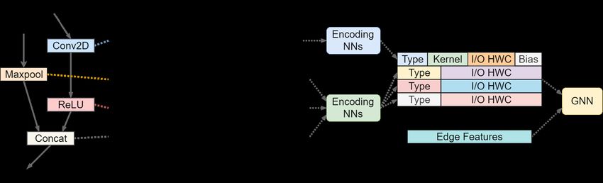
Figure 1: Comparison of architecture representations in neural predictor setups: (a) conventional, space-dependent
neural predictors, e.g., BANANAS and SemiNAS; (b) our proposed, general-purpose, space-agnostic predictor
using Computational Graphs. Best viewed in color.

Bench-201 or NAS-Bench-301 networks. This search-            offer a universal representation of neural architectures
space-specific design severely limits the practicality and   from different search spaces. Figure 1 highlights the
transferability of existing predictors for NAS, since for    differences between (a) existing NAS predictors and (b)
any new search space that may be adopted in reality,         the proposed framework. The key is to introduce a uni-
a separate predictor must be re-designed and re-trained      versal search space representation consisting of graphs
based on a large number of labeled networks in the new       of only primitive operators to model any network struc-
search space.                                                ture, such that a general-purpose transferable predictor
     Another emerging approach to performance estima-        can be learned based on NAS benchmarks available from
tion is ZCP methods, which can support any network           multiple search spaces.
structure as input. However, the performance of ZCPs              Second, we propose a framework to learn a gener-
may vary significantly depending on the search space.        alizable neural predictor by combining recent advances
For example, [2] shows that Synflow achieves a high          in Graph Neural Networks (GNN) [20] and Contrastive
SRCC of 0.74 on the NAS-Bench-201 search space, how-         Learning (CL) [5]. Specifically, we introduce a graph
ever the SRCC drops to 0.37 on NAS-Bench-101. More-          representation learning process to learn a generalizable
over, ZCP methods require the instantiation of a neural      architecture encoder based on the structural informa-
network, e.g., performing the forward pass for a batch       tion of vast unlabeled networks in the target search
of training samples, to compute gradient information,        space. The embeddings obtained this way are then fed
and thus incur longer per-network prediction latency.        into a neural predictor, which is trained based on labeled
In contrast, neural predictors simply require the net-       architectures in the source families, achieving transfer-
work architecture encoding or representation to predict      ability to the target search space.
its performance.                                                  Experimental results on NAS-Bench-101, 201 and
     In general, neural predictors offer better estimation   301 show that our predictor can obtain high SRCC
quality but do not transfer across search spaces, while      on each search space when fine-tuning on no more
ZCPs are naturally universal estimation methods, yet         than 50 labeled architectures in a given target family.
are sub-optimal on certain search spaces. To overcome        Specifically, we outperform several ZCP methods like
this dilemma, in this paper, we propose a general-           Synflow and obtain SRCC of 0.917 and 0.892 on NAS-
purpose predictor for NAS that is transferable across        Bench-201 and NAS-Bench-301, respectively. Moreover,
search spaces like ZCPs, while still preserving the          we use our predictor for NAS with a simple evolutionary
benefits of conventional predictors. Our contributions       search algorithm and have found a high-performance
are summarized as follows:                                   architecture (with 94.23% accuracy) in NAS-Bench-
     First, we propose the use of Computation Graphs to      101 at a low cost of 700 queries to the benchmark,

                                                                                                 Copyright © 2023 by SIAM
                                                                         Unauthorized reproduction of this article is prohibited
outperforming other non-transferable neural predictors 3.1 Abstract Operation Representations With-
such as SemiNAS [17] and BANANAS [32]. Finally, we out the loss of generality, we consider operations in
further apply our scheme to search for an ImageNet [7] neural networks and define a primitive operator as an
network and have found a Once-for-All MobileNetV3 atomic node of computation. In other words, a primitive
(OFA-MBv3) architecture that obtains a top-1 accuracy operator is one like Convolution, ReLU, Add, Pooling
of 79.2% which outperforms the original OFA. or Batch Normalization (BN), which are single points
of execution that cannot be further reduced.
2 Related Work Operator-grouping is an implicit but widely adopted
Neural predictors are a popular choice for perfor- technique for improving the efficiency of NAS. It is a
mance estimation in low-cost NAS. Existing predictor- coarse abstraction where atomic operations are grouped
based NAS works include SemiNAS [17], which adopts and re-labeled according to pre-defined sequences. For
an encoder-decoder setup for architecture encod- example, convolution operations are typically grouped
ing/generation, and a simple neural performance pre- with BN and ReLU [3]. Rather than explicitly rep-
dictor that predicts based on the encoder outputs. Sem- resenting all three primitive operations independently,
iNAS progressively updates an accuracy predictor dur- a simpler representation describes all three primitives
ing the search. BANANAS [32] relies on an ensem- as one grouped operation pattern that is consistent
ble of accuracy predictors as the inference model in its throughout a search space. We can then use these rep-
Bayesian Optimization process. [26] construct a similar resentations as feature inputs to a search algorithm [23,
auto-encoder-based predictor framework and supplies 17] or neural predictor [31, 9], as prior methods do.
additional unlabeled networks to the encoder to achieve While operator grouping provides a useful method
semi-supervised learning. [31] propose a sample-efficientto abstract how we represent neural networks, it hinders
search procedure with customized predictor designs for transferability as groupings may not be consistent across
NAS-Bench-101 and ImageNet [7] search spaces. NPE- search spaces. Take the aforementioned convolution
NAS [30], BRP-NAS [9] are also notable predictor-based example: Although convolutions are typically paired
NAS approaches. By contrast, our approach pre-trains with BN and ReLU operations, the ordering of these
architecture embeddings that are not restricted to a spe-primitives can vary. While NAS-Bench-101 use the
cific underlying search space. ‘Conv-BN-ReLU’ ordering, NAS-Bench-201 use ‘ReLU-
Zero-Cost Proxies (ZCP) are originally proposed as Conv-BN’, thus forming a discrepancy that current
parameter saliency metrics in model pruning techniques. neural predictors do not take into account.
With the recent advances of pruning-at-initialization Compounding this issue, the set of operations can
algorithms, only a single forward/backward propagation differ by search space. While NAS-Bench-101 consid-
pass is needed to assess the saliency. Metrics used in ers Max Pooling, NAS-Bench-201 only uses Average
these algorithms are becoming an emerging trend for Pooling, and NAS-Bench-301 uses complex convolutions
transferable, low-cost performance estimation in NAS. with larger kernel sizes not found in either 101 nor 201.
[2] transfers several ZCP to NAS, such as Synflow [25], A neural predictor trained on any one of these search
Snip [14], Grasp [29] and Fisher [27]. Zero-Cost Proxies spaces using operator-grouping could not easily trans-
could work on any search space and [2] shows that fer to another. Thus, operator-grouping is the main
on certain search spaces, they help to achieve results culprit of low transferability in existing predictors. We
that are comparable to predictor-based NAS algorithms. provide a table enumerating the operator groupings for
However, the performance of ZCPs are generally not each search space in the supplementary materials.
consistent across different search spaces. Unlike neural
predictors such as ours, they require instantation of 3.2 Computational Graphs To construct a neural
candidate networks as well as sample data to compute predictor that is transferable between search spaces,
gradient metrics. we consider a representation that can generalize across
multiple search spaces. We define a Computation Graph
3 A Unified Architecture Representation (CG) as a detailed representation of a neural network
without any customized grouping, i.e., each node in the
In this section, we discuss how to represent neural net-
graph is a primitive operator and the network CG is
works. First, we elaborate on operator-grouping within
made up of only such nodes and edges that direct the
NAS, how it simplifies architecture representation while
flow of information. Without operator-grouping, CGs
hindering transferability between search spaces. Then,
define a search space that could represent any network
we introduce our Computational Graph (CG) frame-
structure since the number of primitive operators is
work and how it solves the transferability problem.
usually far less than the number of possible groupings.
Copyright © 2023 by SIAM
Unauthorized reproduction of this article is prohibitedFigure 2: An example illustrating the key graphical features extracted from compute graphs and how we encode
them as GNN node features. All nodes contain input and output tensor HWC sizes. Nodes with trainable weights
contain additional features on the weight matrix dimensions and bias.
While there are many potential ways to construct primitive operator node and E contains pairs of vertices
a CG, we adopt a simple approach of using the model (vs , vd ) indicating a connection between vs and vd . Un-
optimization graph maintained by deep learning frame- der this definition, the problem of performance estima-
works like TensorFlow [1] or PyTorch [21]. As the name tion becomes finding a function F , e.g., a Graph Neural
suggests, a model optimization graph is originally in- Network (GNN), such that for computation graph Gi ,
tended for gradient calculations and weight updates, which is generated from a candidate neural network,
and it is capable of supporting any network structure. F (Gi ) = Yi , where Yi is the ground truth test score.
In this work, all the CGs used in our experiments are Representing networks as CGs enable us to break
simplified from TensorFlow model optimization graphs. the barrier imposed by search space definitions and
Specifically, we extract the following nodes from a model fully utilize all available data for predictor training,
optimization graph to form a CG: regardless of where a labeled network is from, e.g.,
NAS-Bench-101, 201 or 301. We could also effortlessly
• Nodes that refer to trainable neural network
transfer a predictor trained on one search space to
weights. For these nodes, we extract the atomic
another, by simply fine-tuning it on additional data
operator type, such as Conv1D, Conv2D, Linear,
from the target space.
etc., input/output channel sizes, input/output im-
age height/width sizes, weight matrix dimensions
4 Neural Predictor via Graph Representation
(e.g., convolution kernel tensor) and bias informa-
Learning
tion as node features.
In this section, we propose a two-stage approach to im-
• Nodes that refer to activation functions like ReLU prove generalization and leverage unlabeled data via
or Sigmoid, pooling layers like Max or Average, Contrastive Learning (CL). We first find a vector repre-
as well as Batch Normalization. For these nodes, sentation, i.e., graph embedding, which converts graph
we extract the operator type, input/output channel features with a variable number of nodes into a fixed-
and image height/width sizes. sized latent vector via a graph CL procedure, before
feeding the latent vector to an MLP accuracy regres-
• Key supplementary nodes that indicate how infor-
sor. Given a target family for performance estimation,
mation is processed, e.g., addition, concatentation
a salient advantage of our approach is its ability to lever-
and element-wise multiplication. For these nodes,
age unlabeled data, e.g., computation graphs of the tar-
we also extract the type, input/output channel and
get family, which are typically available in abundance.
image height/width sizes.
In fact, our approach is able to jointly leverage labeled
Figure 2 illustrates how we transform a computa- and unlabeled architectures from multiple search spaces
tion graph into learnable feature vectors. Formally, to maximally utilize available information.
a computation graph G consists of a vertex set V = For each CG Gi , we would like to produce a vector
e
{v1 , v2 , v3 , ...} and an edge set E, where v refers to a representation hi ∈ R for a fixed hyper-parameter e.
Copyright © 2023 by SIAM
Unauthorized reproduction of this article is prohibitedWe would like to infer relationships between networks by Laplacian Eigenvalues
Calculate Topological Similarity
considering the angles between vector representations.
Our CL-based approach learns representations where Computation
Graph
Graph
Encoder
Proj.
MLP
only similar CGs have close vector representations.
Similar Graph Graph
CGs Features Embeddings
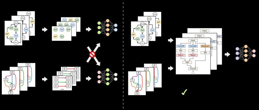
4.1 Contrastive Learning Frameworks Sim-
CLR [5, 6] and SupCon [13] apply CL to image
Computation Graph Proj.
classification. The general idea is to learn a base en- Graph Encoder MLP
coder to create vector representations h of images. To
train the base encoder, a projection head P roj(∗) maps Predictor Features
the vector representations into a lower-dimensional
space z ∈ Rp ; p < e to optimize a contrastive loss.
The contrastive loss forces representations of sim- Figure 3: Contrastive Learning framework. We apply
ilar objects to be in agreement. Consider a batch a graph encoder to produce embeddings. Next, a
of N images, whose vector representation is I = projection layer produces representation vectors whose
{h1 , h2 , . . . , hN } ⊂ Re . For each Gi , let zi = P roj(hi ) ∈ similarity we compare using the CL loss, weighted
{||z|| = 1 : z ∈ Rp }, and let the cosine similarity be according to the Laplacian Eigenvalues of each CG.
sim(zi , zj ) = zi · zj /τ , where the temperature τ > 0
and · is the dot product. The agreement χi,j between
two arbitrary indices i and j is given by 4.2 Computational Graph Encodings Figure 3
provides a high-level overview of our scheme. When ap-
plying CL to CGs, we start by considering the similarity
exp(sim(zi , zj ))
(4.1) χi,j = log P . between CGs. We leverage the rich structural infor-
r6=i exp(sim(zi , zr )) mation CGs provide by encoding each atomic primitive
A primary distinction between SimCLR and SupCon is within a network as a node. Specifically, our approach
how we determine if two different objects are similar. uses spectral properties of undirected graphs [10]. Given
SimCLR considers the unsupersived context where a CG with |V | nodes, we consider its underlying undi-
we do not have access to label/class information. Data rected graph G0 . Let A ∈ {0, 1}|V |×|V | be its adjacency
augmentation plays a crucial role. For each anchor matrix and D ∈ Z|V |×|V | be its degree diagonal matrix.
index i in a batch, we apply a transform or slight The normalized Laplacian matrix is defined as
perturbation to create an associated positive element
j(i), while all other samples r 6= i, j(i) are negative (4.4) ∆ = I − D−1/2 AD−1/2 = U T ΛU,
indices. The SimCLR loss function,
where Λ ∈ R|V |×|V | is the diagonal matrix of eigenvalues
X and U the matrix of eigenvectors. Eigenvalues Λ encode
(4.2) LSimCLR = − χi,j(i) , important connectivity features. For instance, 0 is the
i∈I
smallest eigenvalue and has multiplicity 1 if and only if
0
serves to maximize agreement between the original and G is connected. Smaller eigenvalues focus on general
augmented images. features of the graph, whereas larger eigenvalues focus
By contrast, if classes are known, we can use the on features at higher granularity; we refer the reader to
the SupCon loss function [13], [33] for more details.
More generally, we can use the eigenvalues of ∆ to
X −1 X
(4.3) LSupCon = χi,s , measure pseudo-distance between graphs. Given two
|P (i)| CGs g1 2 , we compute the spectral distance σS (g1 , g2 )
, g
i∈I s∈P (i)
as the Euclidean norm of the corresponding k = 11
where P (i) is the set of non-anchor indices whose class is smallest eigenvalues.
the same as i. Thus, not just j(i), but all indices whose Our constrastive loss incorporates elements from
class is the same as i contribute to the probability of both SimCLR and SupCon in addition to spectral
positive pairs. distance. As our task of interest is regression rather
Next, we construct a contrastive loss for CGs. We than classification, we replace the positive-negative
consider the challenges and advantages of using graphs binary relationship between samples in a batch with a
as data as well as the overall problem of regression probability distribution over all pairs which smoothly
instead of classification. favors similar computation graphs.
Copyright © 2023 by SIAM
Unauthorized reproduction of this article is prohibitedTable 1: Spearman correlation coefficients (ρ). We compare our CL encoding scheme to a GNN encoder as well
as several ZCPs. For our CL and GNN, we report the mean and standard deviation over 5 fine-tuning runs.
Method NAS-Bench-101 NAS-Bench-201 NAS-Bench-301
Synflow [25] 0.361 0.823 -0.210
Jacov [18] 0.358 0.859 -0.190
Fisher [27] -0.277 0.687 -0.305
GradNorm [2] -0.256 0.714 -0.339
Grasp [29] 0.245 0.637 -0.055
Snip [14] -0.165 0.718 -0.336
GNN-fine-tune 0.542 ± 0.14 0.884 ± 0.03 0.872 ± 0.01
CL-fine-tune 0.553 ± 0.09 0.917 ± 0.01 0.892 ± 0.01
First, if the family of networks each CG belongs Bench-201 [8] and NAS-Bench-301 [35], with 50k, 40961
to is known, e.g., NAS-Bench-101, 201, etc., we can and 10k overall CG samples, respectively. We differen-
treat the family affiliation as a class and follow the tiate between target and source families depending on
SupCon approach. Second, rather than using the our configuration. We treat target families as unseen
uniform distribution over P (i) as in Equation 4.3, we use test domains and assume we only have access to a lim-
a convex combination over P (i) based on the similarity ited amount of labeled target data, yet a large amount
of the corresponding computation graphs. Overall, our of unlabeled target CGs. We use source families to train
loss function is given as our predictors and we assume labels are known for each
X X CG.
(4.5) LCL = − αs(i) χi,s , We consider the three cases where one of NAS-
i∈I s∈P (i)
Bench-101, 201 or 301 is the held-out target family, and
(i) P (i) use the other two as source families. We use structural
where αs ≥ 0 and s∈P (i) αs = 1. For computation
information from unlabeled samples in the target family
(i)
graph i, we simply define α∗ to be the softmax of to train our CL encoder in an unsupervised manner.
σS (i, ∗) with temperature 0.05. Then, we use labeled data from the source families
Finally, there are challenges associated with data to train an MLP predictor using supervised regression.
augmentation for CGs. Slightly perturbing a CG may Finally, we use a small amount of labeled data from the
drastically change its accuracy on a benchmark, e.g., target family to fine-tune the MLP predictor.
changing an activation function or convolution [19]. In addition to our CL-based encoder and ZCPs, we
In more severe scenarios, arbitrary small changes to consider a simple GNN [20] regressor baseline that we
a computation graph may make it fall outside of the can train and fine-tune in an end-to-end fashion. We
family of networks of interest or even result in a graph provide implementation details for each predictor in the
that does not represent a functional neural network at supplementary materials.
all. To address this, rather than randomly perturbing a We sample 5k instances from NAS-Bench-101, 4096
CG, we use σ to randomly pick a very similar graph from instances from NAS-Bench-201 and 1k instances from
the training set to form a positive pair. As suggested NAS-Bench-301 when they are the target test family,
in [13], we learn the embeddings using large batch sizes. and use all available data when they are a source family.
We enumerate the structure of our predictor and other When fine-tuning, we use 50 CGs from NAS-Bench-101
details in the supplementary materials. and NAS-Bench-301 and 40 CGs if NAS-Bench-201 is
the target family. We execute the ZCPs on the test sets
5 Experimentation and report the Spearmans Rank Correlation Coefficient
In this section, we evaluate our proposed transferable (SRCC) (ρ ∈ [−1, 1]). SRCC values closer to 1 indicate
predictor by comparing ranking correlations with other higher ranking correlations between predictions and the
transferable Zero-Cost Proxies (ZCP) on popular NAS ground truth accuracy.
benchmarks. Then, we compare with other neural pre- Table 1 summarizes the results. First, we note
dictors in the literature by performing search, show- that our CL-based encoder achieves the best SRCC
ing that methods with higher ranking correlations often in all three target family scenarios. On NAS-Bench-
produce better results. 101, only our CG-based schemes can achieve SRCC
above 0.5, while some ZCPs fail to even achieve positive
5.1 Comparison of ranking correlations We con-
sider the search spaces of NAS-Bench-101 [34], NAS- 1 CIFAR-10 architectures that do not contain ‘zeroize’.
Copyright © 2023 by SIAM
Unauthorized reproduction of this article is prohibitedTable 2: Search results on NAS-Bench-101, 201 and 301 using the same EA search algorithm but with different
performance estimation methods. #Q represents the number of unique networks queried during search. Note
that the #Q for CL-fine-tune also counts the fine-tuning instances.
NAS-Bench-101 NAS-Bench-201 NAS-Bench-301
Method
#Q Acc. (%) Rank #Q Acc. (%) Rank #Q Acc. (%)
Random 700 94.11 ± 0.10 26.0 90 93.91 ± 0.2 104 800 94.75 ± 0.08
Synflow 700 94.18 ± 0.05 5.8 90 94.37 ± 0.0 1.0 800 94.60 ± 0.11
CL-fine-tune 700 94.23 ± 0.01 2.2 90 94.37 ± 0.0 1.0 800 94.83 ± 0.06
correlation. On NAS-Bench-201, only our CL scheme is
Table 3: Search performance of our CL-fine-tuning
able to achieve over 0.9 SRCC while the GNN baseline
predictor and EA search algorithm against other NAS
and the best ZCP methods, Synflow and Jacov, achieve
approaches on NAS-Bench-101. We report the best
around 0.85 SRCC. Similar to [2], on NAS-Bench-301,
architecture accuracy and number of queries.
all of the ZCP schemes fail to achieve positive ranking
correlation. By contrast, both of our predictors achieve NAS algorithm #Queries Best Acc.
over 0.85 SRCC on 301. Moreover, the CL encoder Random Search 2000 93.66%
with fine-tuning achieves very low standard deviation on SemiNAS [17] 2000 94.02%
all three benchmarks. This indicates stable, consistent SemiNAS (RE) [17] 2000 94.03%
performance. Overall, our findings demonstrate the SemiNAS (RE) [17] 1000 93.97%
utility of CGs as generalizable, robust neural network BANANAS [32] 800 94.23%
representations and the capacity of our CL scheme to GA-NAS [23] 378 94.23%
learn rich graph features through unlabeled data. Neural-Predictor-NAS [31] 256 94.17%
NPENAS [30] 150 94.14%
BRP-NAS [9] 140 94.22%
5.2 Search results We now demonstrate that our EA + CL-fine-tune 700 94.23%
predictor is a superior choice for transferable perfor-
mance estimation in NAS. We vary the performance es-
timator and report the accuracy and rank of the best
architecture found. Specifically, we compare the CL- SRCC on NAS-Bench-301 and note how poor estima-
fine-tune predictor for a given target family against the tion performance reflects downstream search results as
Synflow ZCP and a random estimation baseline. We a random estimation baseline outperforms Synflow on
pair each predictor with a simple evolutionary approach that search space. By contrast, with a small amount
that we detail in the supplementary materials. of fine-tuning data, our CL-fine-tune predictor achieves
For each method, we conduct 5 search runs on NAS- exceptional transferability across architecture families
Bench-101 which has 423,624 labeled candidates, NAS- and is able to better guide the search process.
Bench-201 with 15,625 searchable candidates, and NAS- Next, we compare our best search results on NAS-
Bench-301 with over 1018 candidates. To establish a Bench-101 to other state-of-art NAS approaches in
fair comparison, we query (#Q) the same number of Table 3. We observe that our EA + CL-fine-tune setup
networks. Intuitively, the number of queries made to the is competitive with other NAS algorithms. For instance,
benchmark simulates the real-world cost of performance our setup requires fewer queries to find the second-best
evaluation in NAS. architecture (94.23%) in NAS-Bench-101 compared to
Table 2 reports our results. On NAS-Bench-101 and BANANAS. The only other scheme which achieves that
301, our CL-fine-tune predictors consistently find better level of performance is our previous work, GA-NAS [23].
architectures than either Synflow or the random esti- Moreover, our search result is better than SemiNAS in
mation baseline. On average, our CL predictor can find terms of the number of queries and accuracy. It is also
the 2nd best NAS-Bench-101 architecture while Synflow critical to note that, due to the generalizable structure
finds the 6th best, and does not come close in terms of our CGs, we can transfer our predictor to other search
of performance on NAS-Bench-301. On the smallest spaces with only a small amount of labeled data for
search space, NAS-Bench-201, both our CL-fine-tune fine-tuning. This is a unique advantage among neural
predictor and Synflow easily and consistently find the predictors.
best CIFAR-10 architecture. We recall from Table 1 Finally, we further test the efficacy of our predictor
how none of the ZCP methods could achieve positive in NAS by searching on the large-scale classification
dataset ImageNet [7]. To reduce carbon footprint, we
Copyright © 2023 by SIAM
Unauthorized reproduction of this article is prohibitedReferences
Table 4: ImageNet search results. We search in the
OFA-MBv3 space and report the top-1 accuracy ac- [1] Martı́n Abadi et al. TensorFlow: Large-Scale Ma-
quired using the OFA-MBv3 supernet. Most baseline chine Learning on Heterogeneous Systems. 2015.
results are provided by [3]. url: https://www.tensorflow.org/.
[2] Mohamed S. Abdelfattah et al. “Zero-Cost Prox-
Model Top-1 Acc. (%) ies for Lightweight NAS”. In: International Con-
MobileNetV2 [24] 72.0 ference on Learning Representations (ICLR).
MobileNetV2 #1200 [24] 73.5
2021.
MobileNetV3-Large [12] 75.2
NASNet-A [36] 74.0 [3] Han Cai et al. “Once for All: Train One Network
DARTS [16] 73.1 and Specialize it for Efficient Deployment”. In:
SinglePathNAS [11] 74.7 International Conference on Learning Represen-
OFA-Large [3] 79.0 tations. 2020. url: https://openreview.net/
OFA-Base [19] 78.9 forum?id=HylxE1HKwS.
OFA-MBv3-CL 79.2
[4] Liang-Chieh Chen et al. “Deeplab: Semantic Im-
age Segmentation With Deep Convolutional Nets,
Atrous Convolution, and Fully Connected CRFS”.
search on the Once-for-All (OFA) [3] design space for In: IEEE Transactions on Pattern Analysis and
MobileNetV3 (MBv3) [12], which allows us to quickly Machine Intelligence 40.4 (2017), pp. 834–848.
query the accuracy of a found network using a pre-
[5] Ting Chen et al. “A Simple Framework for Con-
trained supernet. We train a CL encoder and predictor
trastive Learning of Visual Representations”. In:
on NAS-Bench-101, 201 and 301, then fine-tune on 50
International Conference on Machine Learning.
random networks from the OFA-MBv3 search space.
PMLR. 2020, pp. 1597–1607.
Table 4 reports our findings. Using the CL predic-
tor, we are able to find an architecture that achieves [6] Ting Chen et al. “Big Self-Supervised Models
over 79.0% top-1 accuracy on ImageNet, outperform- are Strong Semi-supervised Learners”. In: Ad-
ing works on the same search space such as the original vances in Neural Information Processing Systems
OFA [3] and [19]. These results further reinforce the 33 (2020), pp. 22243–22255.
generalizability of our scheme, as we are able to train [7] Jia Deng et al. “ImageNet: A Large-Scale Hierar-
a neural predictor on three CIFAR-10 benchmark fam- chical Image Database”. In: 2009 IEEE Confer-
ilies, then then transfer it to perform NAS on a Mo- ence on Computer Vision and Pattern Recogni-
bileNet family designed for ImageNet. tion. IEEE. 2009, pp. 248–255.
[8] Xuanyi Dong and Yi Yang. “NAS-Bench-201:
6 Conclusion
Extending the Scope of Reproducible Neural
In this work, we propose the use of Computational Architecture Search”. In: International Confer-
Graphs (CG) as a universal representation for CNN ence on Learning Representations (ICLR). 2020.
structures. On top of this representation, we design url: https : / / openreview . net / forum ? id =
a novel, well-performing, transferable neural predictor HJxyZkBKDr.
that incorporates Contrastive Learning to learn robust
[9] Lukasz Dudziak et al. “BRP-NAS: Prediction-
embeddings for a downstream performance predictor.
based NAS Using GCNs”. In: Advances in Neu-
Our transferable predictor alleviates the need to man-
ral Information Processing Systems 33 (2020),
ually design and re-train new performance predictors
pp. 10480–10490.
for any new search spaces in the future, which helps
to further reduce the computational cost and carbon [10] Vijay Prakash Dwivedi and Xavier Bresson.
footprint of NAS. Experiments on the NAS-Bench-101, A Generalization of Transformer Networks to
201 and 301 search spaces verify our claims. Results Graphs. 2021. arXiv: 2012.09699 [cs.LG].
show that our predictor is superior to many Zero-Cost [11] Zichao Guo et al. “Single Path One-shot Neu-
Proxy methods on these search spaces. By pairing our ral Architecture Search with Uniform Sampling”.
predictor with an evolutionary search algorithm we can In: European Conference on Computer Vision.
find a NAS-Bench-101 architecture that obtains 94.23% Springer. 2020, pp. 544–560.
CIFAR-10 accuracy and a MobileNetV3 architecture
that attains 79.2% ImageNet top-1 accuracy.
Copyright © 2023 by SIAM
Unauthorized reproduction of this article is prohibited[12] Andrew Howard et al. “Searching for Mo- [23] Seyed Saeed Changiz Rezaei et al. “Genera-
bileNetv3”. In: Proceedings of the IEEE/CVF tive Adversarial Neural Architecture Search”. In:
International Conference on Computer Vision. Proceedings of the Thirtieth International Joint
2019, pp. 1314–1324. Conference on Artificial Intelligence, IJCAI-21.
[13] Prannay Khosla et al. “Supervised Contrastive Main Track. International Joint Conferences on
Learning”. In: Advances in Neural Information Artificial Intelligence Organization, Aug. 2021,
Processing Systems 33 (2020), pp. 18661–18673. pp. 2227–2234. doi: 10.24963/ijcai.2021/307.
[14] Namhoon Lee, Thalaiyasingam Ajanthan, and [24] Mark Sandler et al. “MobileNetV2: Inverted
Philip HS Torr. “Snip: Single-shot Network Prun- Residuals and Linear Bottlenecks”. In: Proceed-
ing Based on Connection Sensitivity”. In: arXiv ings of the IEEE Conference on Computer Vision
preprint arXiv:1810.02340 (2018). and Pattern Recognition. 2018, pp. 4510–4520.
[15] Liam Li and Ameet Talwalkar. “Random Search [25] Hidenori Tanaka et al. “Pruning Neural Net-
and Reproducibility for Neural Architecture works Without Any Data by Iteratively Conserv-
Search”. In: Uncertainty in Artificial Intelligence. ing Synaptic Flow”. In: Advances in Neural Infor-
PMLR. 2020, pp. 367–377. mation Processing Systems 33 (2020), pp. 6377–
6389.
[16] Hanxiao Liu, Karen Simonyan, and Yiming Yang.
“DARTS: Differentiable Architecture Search”. In: [26] Yehui Tang et al. “A Semi-Supervised Assessor
International Conference on Learning Represen- of Neural Architectures”. In: Proceedings of the
tations (ICLR). 2019. url: http://arxiv.org/ IEEE/CVF Conference on Computer Vision and
abs/1806.09055. Pattern Recognition. 2020, pp. 1810–1819.
[17] Renqian Luo et al. “Semi-Supervised Neural Ar- [27] Jack Turner et al. “Blockswap: Fisher-Guided
chitecture Search”. In: Advances in Neural Infor- Block Substitution for Network Compression on
mation Processing Systems 33 (2020), pp. 10547– a Budget”. In: arXiv preprint arXiv:1906.04113
10557. (2019).
[18] Joe Mellor et al. “Neural Architecture Search [28] Ashish Vaswani et al. “Attention is All You
without Training”. In: International Conference Need”. In: Advances in Neural Information Pro-
on Machine Learning. PMLR. 2021, pp. 7588– cessing Systems 30 (2017).
7598. [29] Chaoqi Wang, Guodong Zhang, and Roger
Grosse. “Picking Winning Tickets Before Training
[19] Keith G Mills et al. “Profiling Neural Blocks
by Preserving Gradient Flow”. In: arXiv preprint
and Design Spaces for Mobile Neural Architecture
arXiv:2002.07376 (2020).
Search”. In: Proceedings of the 30th ACM Inter-
national Conference on Information & Knowledge [30] Chen Wei et al. “NPENAS: Neural Predic-
Management. 2021, pp. 4026–4035. tor Guided Evolution for Neural Architecture
Search”. In: IEEE Transactions on Neural Net-
[20] Christopher Morris et al. “Weisfeiler and Le-
works and Learning Systems (2022).
man Go Neural: Higher-Order Graph Neural Net-
works”. In: Proceedings of the AAAI Conference [31] Wei Wen et al. “Neural predictor for neural archi-
on Artificial Intelligence. Vol. 33. 2019, pp. 4602– tecture search”. In: European Conference on Com-
4609. puter Vision. Springer. 2020, pp. 660–676.
[21] Adam Paszke et al. “PyTorch: An Imperative [32] Colin White, Willie Neiswanger, and Yash Savani.
Style, High-Performance Deep Learning Library”. “BANANAS: Bayesian Optimization with Neural
In: Advances in Neural Information Processing Architectures for Neural Architecture Search”. In:
Systems 32. Ed. by H. Wallach et al. Curran Proceedings of the AAAI Conference on Artificial
Associates, Inc., 2019, pp. 8024–8035. Intelligence. Vol. 35. 12. 2021, pp. 10293–10301.
[22] Hieu Pham et al. “Efficient Neural Architecture [33] Peter Wills and François G Meyer. “Metrics for
Search via Parameters Sharing”. In: International Graph Comparison: A Practitioner’s Guide”. In:
Conference on Machine Learning. PMLR. 2018, Plos one 15.2 (2020), e0228728.
pp. 4095–4104. [34] Chris Ying et al. “NAS-Bench-101: Towards Re-
producible Neural Architecture Search”. In: In-
ternational Conference on Machine Learning.
PMLR. 2019, pp. 7105–7114.
Copyright © 2023 by SIAM
Unauthorized reproduction of this article is prohibited[35] Arber Zela et al. “Surrogate NAS Benchmarks:
Going Beyond the Limited Search Spaces of Tab-
ular NAS Benchmarks”. In: International Con-
ference on Learning Representations. 2022. url:
https : / / openreview . net / forum ? id =
OnpFa95RVqs.
[36] Barret Zoph et al. “Learning Transferable Archi-
tectures for Scalable Image Recognition”. In: Pro-
ceedings of the IEEE Conference on Computer
Vision and Pattern Recognition. 2018, pp. 8697–
8710.
Copyright © 2023 by SIAM
Unauthorized reproduction of this article is prohibitedAlgorithm 1 Evolutionary Search Algorithm (EA)
Table 5: Candidate operation groupings for NAS-
1: Input: Random architecture set P ; Predictor M ;
Bench-101, 201 and 301. We report the sequence
of atomic operations in each grouping as well as the Budget B; NAS-Benchmark D;
2: for t = 1, 2, . . . , T do
number of nodes we would use to represent it as a CG
subgraph. ‘BN’ means Batch Normalization. 3: Pbest ← top-k(P )
4: Pnew ← Mutation and Crossover(Pbest )
Op. Name Sequence #Nodes 5: Pnew ← Rank(Pnew , M ) . Sort using predictor
NAS-Bench-101 [34] 6: Pchild = ∅
1 × 1 Conv [Conv, BN, ReLU] 3 7: for b = 1, 2, . . . , B do
3 × 3 Conv [Conv, BN, ReLU] 3 8: Pchild ← Pchild + Query(Pnew [b], D)
3 × 3 Max Pool [Max Pool] 1 9: end for
NAS-Bench-201 [8] 10: P ← P + Pchild
Zeroize – 0 11: end for
Skip-Connect [Identity] 0
1 × 1 Conv [ReLU, Conv, BN] 3
3 × 3 Conv [ReLU, Conv, BN] 3
3 × 3 Ave. Pool [Ave. Pool] 1 architectures Pbest , and denote them as parent1 and
NAS-Bench-301 [35, 16] parent2 . Then, we randomly select one operator in
Zeroize – 0 parent2 and use it to replace another random operator
Skip-Connect [Identity] 0 in parent1 , ensuring that the selected operator cannot
3 × 3 Sep. Conv* [ReLU, Conv, Conv, BN 8 be the same as the one it is replacing. Therefore, our
ReLU, Conv, Conv, BN] crossover is single-point and uniformly random. After
5 × 5 Sep. Conv* [ReLU, Conv, Conv, BN 8 crossover, we perform additional mutations on the child
ReLU, Conv, Conv, BN] architecture.
3 × 3 Dil. Conv† [ReLU, Conv, Conv, BN] 4 In the mutation procedure, we select architectures
5 × 5 Dil. Conv† [ReLU, Conv, Conv, BN] 4
that are members of Pbest or that came from the
3 × 3 Ave. Pool [Ave. Pool] 1
3 × 3 Max Pool [Max Pool] 1
crossover procedure and perform 1-edit random muta-
tions on their internal structures. The actual definition
* Depthwise Separable Convolution [24]. The first
for 1-edit change is determined by the search space. For
convolution in a ‘Conv, Conv’ pair has ‘groups’ equal
to input channels, and the second conv is 1 × 1.
example, on NAS-Bench-101, 1-edit mutations include
† Dilation (Atrous) Convolution [4]. The first conv in a the following:
pair has a dilated kernel, while the second is 1 × 1.
• Swap an existing operator in the cell with another
uniformly sampled operator.
7 Supplementary Materials • Add a new operator to the cell with random
7.1 Architecture Groupings Table 5 enumerates connections to other operators.
the operator groupings for NAS-Bench-101, NAS-
Bench-201 and NAS-Bench-301, respectively. Further- • Remove an existing operator in the cell and all of
more, we list the number of nodes a Computational its incoming/outgoing edges.
Graph (CG) needs to encode each sequence. Finally, we
• Add a new edge between two existing operators in
note the presence of depthwise separable [24] and dilated
the cell.
(atrous) convolutions [4] in NAS-Bench-301, in contrast
to the regular convolutions found in NAS-Bench-101 • Remove an existing edge from the cell.
and NAS-Bench-201.
It is also worth mentioning that in our search we allow
7.2 Evolutionary Search To perform search, we for more than 1-edit mutations, i.e., we could randomly
adopt a common Evolutionary Algorithm (EA) that perform consecutive mutations on an architecture to
consists of a combination of crossover and mutation boost the diversity of the new population Pnew .
procedures to create a larger pool of child architectures. We evaluate the performance of each architecture
We provide a high-level description for our procedure. in Pnew using a given performance predictor M . We
Given a population of architectures P , at each denote a NAS-Benchmark we can query as D as well
iteration t = 1, 2, . . . , T , we select the current top-k as a query budget B. Using D, we query the ground
best architectures as potential parents and denote this truth performance of the first B architectures in Pnew
subset as Pbest . To perform crossover, we select two and denote this labelled subset Pchild . We add Pchild
Copyright © 2023 by SIAM
Unauthorized reproduction of this article is prohibitedTable 6: Summary of key hyper-parameters for our EA search algorithm. Pinit refers to the starting population.
NAS-Bench-101 NAS-Bench-201 NAS-Bench-301
Method
k B |Pinit | T k B |Pinit | T k B |Pinit | T
Random/Synflow 20 100 100 6 10 20 10 4 20 100 100 7
CL-fine-tune 20 100 50 6 10 10 10 5 20 100 50 7
to the existing population P and continue to the next
iteration t + 1. Algorithm 1 summarizes our overall
search procedure, while Table 6 enumerates our specific
hyperparameter settings.
7.3 Predictor Components Our CL graph encoder
considers Transformer [28] attention mechanisms with
positional embeddings [5, 6] to capture global graph
relationships and k-GNN [20] layers to capture local
features. Starting from operation node embeddings,
the transformer encoder consists of up to 2 layers with
2 attention heads, whose output we concatenate with
a k-GNN [20] to form an overall graph embedding of
size m = 128. We generate graph embeddings by
aggregating the features of all nodes using the mean
operation. An MLP with 4 hidden layers and ReLU
projects the graph embedding down to size p = 64 to
compute the CL loss. When training the CL encoder,
we set τ = 0.1 and normalize output representations as
[13] suggest. Finally, we use a separate MLP head with
5 layers and a hidden size of 200 to make a prediction
from the CL embedding.
Our simple GNN graph encoder baseline consists of
4 or 6 layers with node feature size 64. We apply the
same mean aggregation to form a graph embedding, and
then use an MLP head with 4 hidden layers and ReLU
activation to make a prediction.
Copyright © 2023 by SIAM
Unauthorized reproduction of this article is prohibitedYou can also read