A look ahead Monte Carlo simulation method for improving parental selection in trait introgression - Nature
←
→
Page content transcription
If your browser does not render page correctly, please read the page content below
www.nature.com/scientificreports
OPEN A look‑ahead Monte Carlo
simulation method for improving
parental selection in trait
introgression
Saba Moeinizade1, Ye Han2, Hieu Pham2, Guiping Hu1* & Lizhi Wang1
Multiple trait introgression is the process by which multiple desirable traits are converted from a
donor to a recipient cultivar through backcrossing and selfing. The goal of this procedure is to recover
all the attributes of the recipient cultivar, with the addition of the specified desirable traits. A crucial
step in this process is the selection of parents to form new crosses. In this study, we propose a new
selection approach that estimates the genetic distribution of the progeny of backcrosses after multiple
generations using information of recombination events. Our objective is to select the most promising
individuals for further backcrossing or selfing. To demonstrate the effectiveness of the proposed
method, a case study has been conducted using maize data where our method is compared with state-
of-the-art approaches. Simulation results suggest that the proposed method, look-ahead Monte Carlo,
achieves higher probability of success than existing approaches. Our proposed selection method can
assist breeders to efficiently design trait introgression projects.
From a commercial breeding perspective, trait introgression (TI) is a necessary process to produce the elite culti-
var with the most desirable traits. This technique is used to incorporate desired traits from a donor into an exist-
ing elite cultivar, preserving the performance of the elite cultivar and adding the benefits of the introduced traits.
The result is essentially the same elite cultivar with the added desired traits that will bring benefits to growers1.
As an illustration, imagine two maize populations: one population (recipient) characterized by high yielding
potential and low resistance to drought stress, whereas the other population (donor) characterized by low yield
potential and high resistance to drought stress. In this scenario, one would hope to recover all the attributes of
the recipient while obtaining the drought resistant alleles of the donor by some mechanized breeding process
to create a new elite cultivar.
Marker-assisted backcrossing strategies provide important time and quality advantages over classical pro-
cedures for introgression of desirable alleles from a donor to an elite c ultivar2–6. Backcrossing is a well-known
breeding approach for the introgression of a target gene from a donor cultivar into the genomic background of a
recipient cultivar3–5,7,8. The donor parent (DR) provides the desired trait and may not perform as well as an elite
variety in other areas. The elite cultivar, called the recurrent parent (RP), usually performs well in the background.
The objective is to increase the recipient genome content of the progenies, by repeated backcrosses to the recipient
cultivar to recover all the attributes of the recipient cultivar, with the addition of the specified desirable traits9.
Although, in principle, the intent of trait introgression is forthright, in practice, there exists many compli-
cations due to the stochastic nature and size of a commercial breeding program. Because of this uncertainty,
multiple breeding generations may be required until the superior, desired cultivar is achieved10. An additional
challenge of the TI process is selecting the most promising backcross individuals for further backcrossing or
selfing4,7. At each backcross generation cycle, plant breeders are faced with the difficult decision of identifying
crosses to perform to produce the next generation of, hopefully, superior cultivar. In the prefect scenario, plant
breeders would be able to cross every possible combination of parents until the desired cultivar is achieved. How-
ever, in reality, due to the limited amount of available resources (time, money, land, technology, etc.), breeders
may only consider a small fraction of an existing gene pool, possibly leading to sub-optimal decision making11–13.
Recent advances in simulation and optimization techniques have been applied to variety of disciplines includ-
ing plant breeding14–20. Computer simulation approaches help identify optimal breeding strategies by adopting
assumptions of the breeding system and running multiple scenarios, whereas, optimization approaches aim to
1
Industrial and Manufacturing Systems Engineering, Iowa State University, Ames, IA 50011, USA. 2Syngenta,
Slater, IA 50244, USA. *email: gphu@iastate.edu
Scientific Reports | (2021) 11:3918 | https://doi.org/10.1038/s41598-021-83634-x 1
Vol.:(0123456789)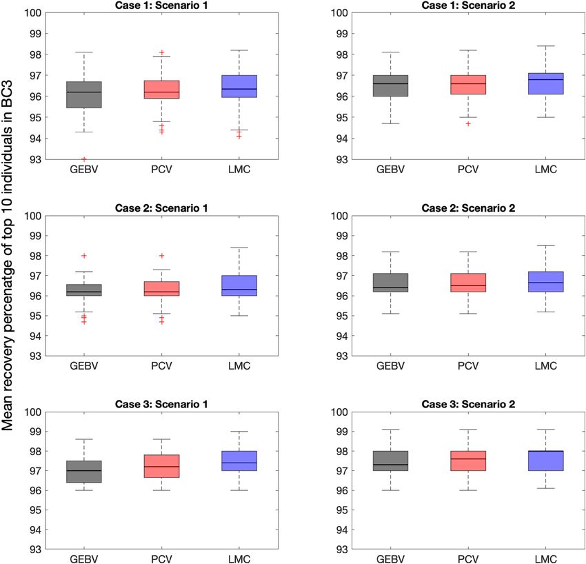
www.nature.com/scientificreports/
produce the best framework to maximize the probability of achieving the desired cultivar while minimizing
input resources. It should be noted that the combination of analytical techniques and plant breeding has mainly
been applied to genomic selection and not trait i ntrogression21–27.
Although there does not currently exist much literature to integrate operations research techniques and trait
introgression, there are still a few impactful studies. Cameron et al. utilized an operations research framework
with a stochastic optimization model to identify the best breeding strategies for a given population under resource
constraints28. This work illustrates the potential optimization modeling can have on resource allocation in plant
breeding. Probabilistic simulation techniques have also been performed by Sun and M umm29 to assess in silico
30
various crossing schemes and breeding approaches. Moreover, Han et al. has framed trait introgression as
an algorithmic process and introduced a novel selection metric, predicted cross value (PCV), which predicts
specific combining ability by estimating the probability that a pair of parents will produce a perfect gamete with
all desirable alleles.
Due to the importance of optimizing the breeding pipeline and the need to consider resource limitations for
large scale breeding programs, this paper aims to design a platform that integrates operations research methods
to trait introgression. Specifically, the authors develop a novel Monte Carlo simulation approach for the TI pipe-
line to consider the parental selection aspect under different scenarios of resources present within a commercial
scale TI program. The originality in the proposed method, look-ahead Monte Carlo (LMC), is to look ahead and
estimate the performance of progeny in the target generation and then optimize the selection decisions based
on the estimated performance. In this study, we use computer simulations to compare selection strategies with
respect to the recurrent parent background gene recovery percentage of individuals in the final generation.
Methods
In this section, we first define the problem by describing the backcrossing breeding pipeline and introduce two
existing selection methods. Then, we propose the novel look-ahead Monte Carlo selection method.
Problem definition. The following abbreviations will be used in subsequent sections in this paper:
DR: donor RP: recurrent parent
BCt: backcross population at generation t
BCTF2: self-fertilized population after final backcross
GEBV: genomic estimated breeding value
PCV: predicted cross value
LMC: look-ahead Monte Carlo
The general objective of trait introgression projects is to produce a new line that is highly close to the recurrent
parent, and contains the desired alleles or traits from the donor parent. First an initial cross is made between the
donor and recurrent parent to produce F1 progeny. Since, the donor and recurrent parents are both homozy-
gous, this step is deterministic which means the F1 progeny has 50% of the genetic material from each parent.
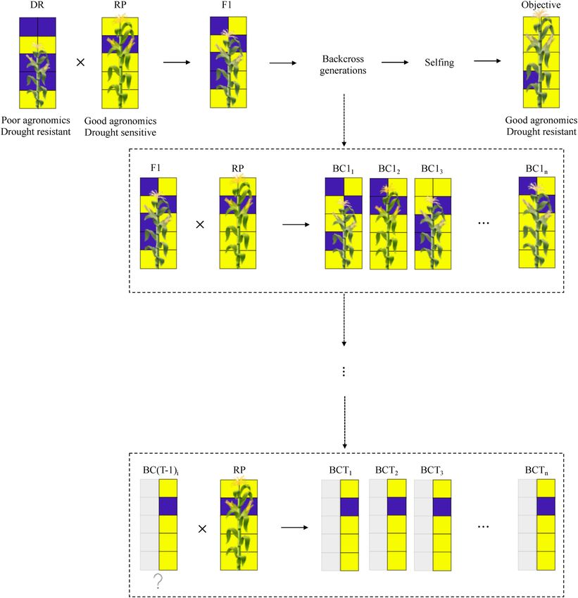
Next, the F1 individual is crossed to the recurrent parent to develop a backcross one (BC1) population. Figure 1
represents a schematic overview of the backcross project where the ultimate goal is to produce drought resistant
individual plants with good agronomics. In Fig. 1, we see n individuals in the backcross one population denoted
with BC11 , BC12 , ..., and BC1n . Best individuals from the BC1 population were selected based on a selection
strategy and then again backcrossed to the recurrent parent.
In successive generations, progeny are first selected for the trait of interest and then backcrossed to the recur-
rent parent. This process is repeated for T backcross generations. We refer to an individual as positive if it contains
the desirable alleles from the donor. For positive individuals in BCT population, the percentage of beckground
recovery was calculated by dividing the number of desirable alleles in the background by the total number of
background alleles. Furthermore, we monitor and evaluate the BCTF2 individuals.
The donor parent (poor agronomics, drought resistant) is crossed with the recurrent parent (good agronomics,
drought sensitive) to produce F1. F1 progeny have 50% of their genetic material from each parent (yellow square:
favorable allele, purple square: unfavorable allele). Then, F1 is backcrossed with the recurrent parent to develop
the BC1 population. Best individuals from BC1 are selected based on a predefined metric and backcrossed to the
recurrent parent. This process is repeated for T generations. The ultimate goal is to achieve an individual which
is drought resistant and has good agronomics.
To simulate the recombination process during meiosis we used the same inheritance distribution defined i n30.
In subsequent sections, the recombination frequency vector is denoted by r ∈ [0, 0.5]L−1, where L is the total
number of markers in the genome. To represent the genotype of an individual plant, we use an L × m binary
matrix, say G ∈ BL×m, where Gl,m = 1 indicates whether the l th allele from chromosome m is desirable or not
(Gl,m = 0). For each individual plant represented with a binary matrix, each row is a locus in the genome. The
number of columns in the binary matrix represents the ploidy of the plant. We use diploid species in this paper
(m = 2). Here, we review two existing approaches for parental selection.
Background selection. The background selection approach first selects the individuals with desired marker gen-
otypes and then among these positive individuals selects for the desired background g enotype3,7,31. Background
selection has been shown to be efficient by previous theoretical w ork3,31–33 and experimental work2.
The breeding value of a background genotype can be estimated using genomic estimated breeding value
(GEBV)34,35. GEBV of individual plants (or animals) is defined as the sum of their estimated marker e ffects34. We
assume D = {d1 , d2 , ..., dz } is the location of the positive markers from the donor and there are total Z markers
that should be introgressed. If we assume uniform weight for all desirable alleles, then the background GEBV of
an individual is equivalent to the number of desirable alleles in its background:
Scientific Reports | (2021) 11:3918 | https://doi.org/10.1038/s41598-021-83634-x 2
Vol:.(1234567890)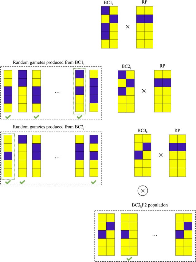
www.nature.com/scientificreports/
Figure 1. A schematic overview of the backcross project.
L
2
GEBV = Gl,m
m=1 (1)
l=1
l∈
/D
According to this approach, the positive individuals with highest GEBVs will be selected as parents.
Predicted cross value selection. The predicted cross value (PCV) calculates the probability that a pair of breed-
ing parents will produce a gamete with desirable alleles at all specified loci by taking into account the recombi-
nation frequencies30. This approach selects individuals based on their likelihood to produce an elite gamete by
combining all desirable alleles. Since in a backcrossing scheme, individuals are always crossed with the recurrent
parent, the PCV can be defined as the probability that each individual will produce an elite gamete.
Let g ∈ BL×1 denote a random gamete produced by a breeding parent. The PCV of an individual is calculated
as follows:
Scientific Reports | (2021) 11:3918 | https://doi.org/10.1038/s41598-021-83634-x 3
Vol.:(0123456789)www.nature.com/scientificreports/
PCV (G, r) = Pr(gi = 1, ∀i ∈ {1, 2, ..., L}) (2)
25
To calculate this probability, the same water-pipe algorithm described in is used. The rationale for the PCV
eiosis30.
definition is to calculate the probability that none of the undesirable alleles survives two generations of m
According to this approach, the positive individuals with highest PCVs will be selected as parents.
Proposed look‑ahead Monte Carlo algorithm. In this section we propose a novel probabilistic and
heuristic driven search algorithm, look-ahead Monte Carlo (LMC) for parental selection. The underlying con-
cept is to use Monte Carlo simulation for modeling uncertainty involved due to recombination events. Monte
Carlo simulation is a technique that relies on repeated random sampling to obtain numerical results36. This tech-
nique is often used in physical and mathematical problems and is most suited to be applied when it is impossible
to obtain a closed-form expression or infeasible to apply a deterministic algorithm37.
The look-ahead Monte Carlo algorithm for parental selection evaluates different selection decisions periodi-
cally during the learning phase by predicting the genetic distribution of the progeny of backcrosses after multiple
generations using information of recombination events. This algorithm makes a trade-off between exploration
and exploitation. It exploits the selection strategies that is found to be best until the current generation and also
explores the alternative decisions to find out if they could replace the current best. The essence of this algorithm
is to strategically search the space to find optimal crosses that can result in best performance in the targeted
generation.
Figure 2 presents an overview of the LMC algorithm. For every individual in BCt population (e.g., BCti ),
multiple random gametes are simulated according to the recombination frequencies. These gametes are narrowed
down to the ones which have the desirable markers from the donor in the introgressed loci. Then, one of these
positive gametes is selected randomly to form the next BC progeny (e.g., BC(t+1)i ). This process is repeated until
the target generation (BCT). Finally, individuals are evaluated based on their performance after selfing (BCTF2).
In BCTF2, success can be defined as achieving certain amount of recovery percentage (e.g., 95%) among
positive individuals. Suppose the population size of the BCTF2 generation is K and n individuals with desirable
markers have achieved the desired recovery percentage. Then Kn is the probability of getting a positive individual
that has met the background recovery requirements. Since through backcross generations the gametes are selected
randomly, this probability is estimating only one of the possible outcomes for individual i in BCt population. To
have a reasonable approximation for the performance of progeny in BCTF2, the same process should be repeated
multiple times. The objective of the LMC algorithm can then be calculated as:
P n j j
j=1 K v (3)
Q=
P
where v j represents the maximum recovery percentage achieved in BCTF2 for the jth round, and P is total rounds
of repetition. According to LMC approach, individuals with highest Q values will be selected as the breeding
parents.
Results
In this section, we first describe the data sets used in this case study, and then compare the proposed method
with two existing selection methods in different scenarios of resources using computer simulation.
Data. Data contains donor and recipient’s genetic information and recombination frequencies. To explore
the effect of having different initial genetic similarities between donor and recurrent parent, we considered three
cases as demonstrated in Table 1. The genetic similarity is calculated based on the NEIs metric38. Cases 1, 2, and
3 have low, moderate and high initial genetic similarities respectively. Our goal is to compare the performance
of selection strategies using these 3 different cases given that the low initial genetic similarity (case 1) is expected
to be more difficult relatively.
The genetic information of donor and recurrent parent for these three cases are illustrated in Fig. 3. For all
cases, three markers should be integrated from the donor to the recurrent parent. Furthermore, the recombina-
tion events are presented in the supplementary information.
Simulation settings. Multiple trait introgression was studied using realistic maize data with three different
selection methods, including GEBV, PCV, and LMC. We considered three cases with different genetic similari-
ties and two different scenarios for resources. These scenarios are designed considering the practical aspects of
a breeding program. In scenario 1, we are allocating limited resources by making 2 crosses in each generation
whereas in scenario 2, we are allocating moderate resources by making 6 crosses in each generation (see Table 2).
Scenario 1 more closely resembles what occurs in a commercial breeding program, namely, decision making
with limited resources.
One hundred independent simulation replicates were performed for each of the selection methods using
MATLAB (R2019-a). Simulation has been performed for three generations of backcrosses followed by a selfing.
The evaluation is based on the recovery percentage of individuals in BC3F2 generation.
It is assumed that each cross makes 200 progeny and for each scenario the number of crosses remains the
same through all generations (i.e. resources are distributed evenly among different generations).
Simulation results. Comparison of selection methods for one sample simulation Figure 4 presents the perfor-
mance of three selection methods for one sample simulation. The histograms of background recovery percentage
Scientific Reports | (2021) 11:3918 | https://doi.org/10.1038/s41598-021-83634-x 4
Vol:.(1234567890)www.nature.com/scientificreports/
Figure 2. The Monte Carlo search for parental selection in trait introgression. For a deadline of T generations,
we estimate the performance of BCTF2 individuals for a given selection strategy by searching across all possible
paths. This is a schematic overview of monitoring the estimated performance in BC3F2 for a single path. The
same process is repeated multiple times and then the average value is assigned to BC1i.
Case NEIs (%) Number of markers
1 0.58 195
2 0.72 173
3 0.89 172
Table 1. The description of data sets.
for positive individuals are demonstrated over BC1, BC2, BC3, and BC3F2 generations. All three methods start
with the same BC1 population and then produce the next population based on different selection decisions. As
expected, the background recovery improves from BC1 to BC3 for all selection methods. For this sample simula-
tion, the (maximum, mean, minimum) recovery percentage in BC3 is (94, 90.61, 85), (94, 89.71, 84), (97, 94.07,
Scientific Reports | (2021) 11:3918 | https://doi.org/10.1038/s41598-021-83634-x 5
Vol.:(0123456789)www.nature.com/scientificreports/
DR RP r DR RP r DR RP r
0.5 0.5 0.5
0.45 0.45 0.45
0.4 0.4 0.4
0.35 0.35 0.35
0.3 0.3 0.3
0.25 0.25 0.25
0.2 0.2 0.2
0.15 0.15 0.15
0.1 0.1 0.1
0.05 0.05 0.05
Figure 3. Donors and recurrent parents’ genetic information and recombination frequencies for three cases
(DR: donor, RP: recurrent parent, r: recombination frequency). A yellow square is used to denote a favorable
allele (“1”) and a purple square is used to denote an unfavorable allele (“0”). The gray charts are heat maps for
recombination frequencies.
Scientific Reports | (2021) 11:3918 | https://doi.org/10.1038/s41598-021-83634-x 6
Vol:.(1234567890)www.nature.com/scientificreports/
Generation Scenario 1 (limited resources) Scenario 2 (moderate resources)
BC1 2 6
BC2 2 6
BC3 2 6
Table 2. Numbers of crosses in each generation for two different scenarios.
Figure 4. A sample simulation result for three different selection methods presenting histograms of population
background recovery percentage over different generations. This simulation is performed for case 2, scenario 1.
92) for GEBV, BPV, and LMC methods respectively which demonstrates improvement in recovery percentage
when selection decisions are made using the LMC method.
It should be noted that the BC3F2 individuals should have all 6 alleles desirable in the three markers that
are to be integrated from the donor (i.e. BC3F2 individuals are homozygous). However, the BC individuals are
expected to have 3 desirable alleles total since their second chromosome is being inherited from the recurrent
parent. This can explain why recovery percentage drops from BC3 to BC3F2. As demonstrated in Fig. 4, for this
sample simulation, the LMC method achieves 95% recovery in BC3F2, however the other two selection methods
achieve maximum 91% recovery.
Background recovery percentage of the top individual in BC3 across all simulation replicates Figure 5 compares
the cumulative distribution functions (CDFs) of maximum recovery percentage achieved in BC3 for three selec-
tion methods among 100 simulation replicates. The further toward the right direction a CDF curves, the better
performance a method has. Take for example, point (97, 75) means that 75% of the simulations have achieved
recovery percentage less than or equal to 97. In all cases and scenarios, the LMC method achieves higher recov-
ery percentage.
Scientific Reports | (2021) 11:3918 | https://doi.org/10.1038/s41598-021-83634-x 7
Vol.:(0123456789)www.nature.com/scientificreports/
GEBV PCV LMC
Case 1: Scenario 1 Case 1: Scenario 2
100% 100%
90% 90%
80% 80%
70% 70%
60% 60%
50% 50%
40% 40%
30% 30%
20% 20%
10% 10%
0% 0%
94 95 96 97 98 99 100 94 95 96 97 98 99 100
Case 2: Scenario 1 Case 2: Scenario 2
100% 100%
90% 90%
80% 80%
Cumalative frequency
70% 70%
60% 60%
50% 50%
40% 40%
30% 30%
20% 20%
10% 10%
0% 0%
94 95 96 97 98 99 100 94 95 96 97 98 99 100
Case 3: Scenario 1 Case 3: Scenario 2
100% 100%
90% 90%
80% 80%
70% 70%
60% 60%
50% 50%
40% 40%
30% 30%
20% 20%
10% 10%
0% 0%
94 95 96 97 98 99 100 94 95 96 97 98 99 100
Recovery percentage in BC3
Figure 5. Cumulative distribution functions of population maximum in the BC3 for three cases and two
different scenarios. Results are based on 100 simulation replicates.
For case 3 which has the highest genetic similarity between donor and recurrent parent, there was one simula-
tion that resulted in having one individual in BC3 with all desirable traits (100% recovery percentage). Note that
since this is a backcross generation, for this individual the second chromosome still lacks the desirable alleles
from the donor. As expected, for each case, scenario 2 has better performance compared to scenario 1 since
there are more resources available.
Average background recovery percentage of top 10 individuals in BC3 across all simulation replicates Figure 6
presents the box-plots of average recovery percentage of top 10 individuals in BC3 generation. For all cases and
scenarios, the median value is higher when selection decisions are optimized using LMC method. Furthermore,
PCV has generally higher median values than GEBV. The overall range of values is greater for LMC method (as
shown by the distances between the ends of the two whiskers for each box-plot). The interquartile ranges are
reasonably similar (as shown by the lengths of the boxes), except for case 2, scenario 1, where LMC has consid-
erably higher range.
Background recovery percentage of the top individual in BC3F2 across all simulation replicates Figure 7 com-
pares the probability of success for three selection methods by evaluating recovery percentage of best individual
in BC3F2. For example, point (0.8, 95) means that 80% of the simulations have achieved recovery percentage of
Scientific Reports | (2021) 11:3918 | https://doi.org/10.1038/s41598-021-83634-x 8
Vol:.(1234567890)www.nature.com/scientificreports/
Figure 6. Box-plots of mean recovery percentage of top 10 individuals in BC3 for three selection methods. For
each case and scenario, 100 simulation replicates are performed. The median values are demonstrated with a
bold line.
95 in the terminal generation. The curves with better performance are expected to be closer to the upper right
corner of the plot.
As expected, scenario 2 has generally higher probability of success compared to scenario 1 as more resources
are used. Take for example, for case 2 the probability of achieving 95 percentage recovery with LMC method
increases from 0.74 to 0.83 when having more resources. This probability also increases from 0.59 to 0.71 for
PCV and from 0.54 to 0.69 for GEBV method. Furthermore, the probability of success increases from case 1 to
3 where there is more genetic similarity between the donor and parent. Take scenario 2 for example, the prob-
abilities of having 95 percentage recovery when selection decisions are optimized using LMC method are 0.81,
0.83, 0.89 for cases 1, 2, and 3, respectively.
Discussion
Selection methods based on marker information make trait introgression more efficient and effective. When
introgressing the desired traits form a donor to a recipient, background selection is the conventional selection
approach that aims to recover the desired background genome. Recent advances in optimization and simulation
techniques can help enhancing the efficiency of parental selection in breeding programs.
Scientific Reports | (2021) 11:3918 | https://doi.org/10.1038/s41598-021-83634-x 9
Vol.:(0123456789)www.nature.com/scientificreports/
GEBV PCV LMC
Case 1: Scenario 1 Case 1: Scenario 2
100 100
99 99
98 98
97 97
96 96
95 95
94 94
93 93
92 92
91 91
90 90
0 0.2 0.4 0.6 0.8 1 0 0.2 0.4 0.6 0.8 1
Recovery percentage in BC3F2
Case 2: Scenario 1 Case 2: Scenario 2
100 100
99 99
98 98
97 97
96 96
95 95
94 94
93 93
92 92
91 91
90 90
0 0.2 0.4 0.6 0.8 1 0 0.2 0.4 0.6 0.8 1
Case 3: Scenario 1 Case 3: Scenario 2
100 100
99 99
98 98
97 97
96 96
95 95
94 94
93 93
92 92
91 91
90 90
0 0.2 0.4 0.6 0.8 1 0 0.2 0.4 0.6 0.8 1
Probability of success Probability of success
Figure 7. Probability of success in BC3F2 for three different selection approaches considering 3 cases of initial
genetic similarity and 2 scenarios of resource allocation for 100 simulation replicates. The maximum recovery
percentage of positive individuals in BC3F2 is first identified and then probability of success has been defined as
the proportion of simulations that have achieved a certain recovery.
In this study, we introduced a new selection method, LMC, which has the potential to further improve the
efficiency of breeding given limited time and resources by integrating operations research techniques and trait
introgression. The proposed method was compared with existing selection methods in a simulation study using
empirical maize data. Computational results demonstrate the improvements of the LMC method over two exist-
ing selection approaches, GEBV and PCV.
One of the advantages of the LMC method is being sensitive to the deadline. Unlike other selection meth-
ods that evaluate the performance based on only next generation, the LMC method relates the objective to the
performance of individuals in the targeted generation. Another advantage of the LMC method is the trade-off
between exploration and exploitation. When the look ahead process finds exploitation to contribute more to the
final objective, the algorithm behaves in a greedy way to maximize performance. However, when the exploration
is found to be more beneficial, the algorithm explores new possible outcomes.
Scientific Reports | (2021) 11:3918 | https://doi.org/10.1038/s41598-021-83634-x 10
Vol:.(1234567890)www.nature.com/scientificreports/
The simulations in this study were designed based on practical considerations. The trait introgression pipeline
included three backcross generations followed by a selfing so that selected individuals will be homozygous for
the target trait. There is no absolute number for the number of backcrosses needed to be performed but generally
between two to five backcrosses are performed in maize. The number of required generations can be determined
based on the breeding objective and the resources invested at each g eneration39. Intuitively, making more crosses
and producing more progeny leads to a higher chance of creating desirable individuals, however the resources
are limited and the breeding strategy should be customized based on available resources. Here, we considered
two scenarios to represent both limited and moderate cases of resource availability. Scenario 1 limits the number
of crosses to two in each generation where as scenario 2 allows six crosses. According to reproductive biology of
maize, it is possible to obtain ≈ 200 seeds from a cross. Thus, we assumed each cross makes 200 progeny which
means for scenarios 1 and 2, the population size of each generation becomes 400 and 1200 respectively. As
expected, simulation results demonstrated that the probability of success increases when having more resources.
Future work should investigate optimizing the resource allocation strategies by spreading out the budget
systematically among different generations. Also, this study investigated introgressing desirable alleles from a
single donor, however desirable alleles can be carried by multiple donors. Hence, another direction that deserves
investigation is to extend the LMC method for the cases with multiple donors. Moreover, we based our simula-
tions on a single crop organism. Further simulations considering more diverse populations are necessary to
demonstrate the general applicability of the proposed selection method.
Received: 2 September 2020; Accepted: 14 January 2021
References
1. Ødegård, J. et al. Incorporating desirable genetic characteristics from an inferior into a superior population using genomic selec-
tion. Genetics 181, 737–745 (2009).
2. Ragot, M. et al. Marker-assisted backcrossing: a practical example. in COLLOQUES-INRA 45–45 (1995).
3. Visscher, P. M., Haley, C. S. & Thompson, R. Marker-assisted introgression in backcross breeding programs. Genetics 144, 1923–
1932 (1996).
4. Frisch, M. & Melchinger, A. E. Selection theory for marker-assisted backcrossing. Genetics 170, 909–917 (2005).
5. Khan, G. H. et al. Marker-assisted introgression of three dominant blast resistance genes into an aromatic rice cultivar Mushk
Budji. Sci. Rep. 8, 1–13 (2018).
6. Sun, X. & Mumm, R. H. Optimized breeding strategies for multiple trait integration: III. Parameters for success in version testing.
Mol. Breed. 35, 201 (2015).
7. Frisch, M., Bohn, M. & Melchinger, A. E. Comparison of selection strategies for marker-assisted backcrossing of a gene. Crop Sci.
39, 1295–1301 (1999).
8. Peng, T., Sun, X. & Mumm, R. H. Optimized breeding strategies for multiple trait integration: I. Minimizing linkage drag in single
event introgression. Mol. Breed. 33, 89–104 (2014).
9. Bouchez, A. et al. Marker-assisted introgression of favorable alleles at quantitative trait loci between maize elite lines. Genetics 162,
1945–1959 (2002).
10. Wang, X., Wang, Y., Zhang, G. & Ma, Z. An integrated breeding technology for accelerating generation advancement and trait
introgression in cotton. Plant Breed. 130, 569–573 (2011).
11. Allier, A., Moreau, L., Charcosset, A., Teyssèdre, S. & Lehermeier, C. Usefulness criterion and post-selection parental contributions
in multi-parental crosses: Application to polygenic trait introgression. G3 Genes Genomes Genet. 9, 1469–1479 (2019).
12. Twyford, A. & Ennos, R. Next-generation hybridization and introgression. Heredity 108, 179–189 (2012).
13. Dempewolf, H. et al. Past and future use of wild relatives in crop breeding. Crop Sci. 57, 1070–1082 (2017).
14. Li, X., Zhu, C., Wang, J. & Yu, J. Computer simulation in plant breeding. in Advances in agronomy, vol. 116, 219–264 (Elsevier,
Amsterdam, 2012).
15. Shahhosseini, M., Martinez-Feria, R. A., Hu, G. & Archontoulis, S. V. Maize yield and nitrate loss prediction with machine learning
algorithms. Environ. Res. Lett. 14, 124026 (2019).
16. Ansarifar, J., Akhavizadegan, F. & Wang, L. Performance prediction of crosses in plant breeding through genotype by environment
interactions. Sci. Rep. 10, 1–11 (2020).
17. Shahhosseini, M., Hu, G., Archontoulis, S. V. & Huber, I. Coupling machine learning and crop modeling improves crop yield
prediction in the us corn belt. arXiv:2008.04060 (2020).
18. Hosseini, S. A., Alhasan, A. & Smadi, O. Use of deep learning to study modeling deterioration of pavements a case study in Iowa.
Infrastructures 5, 95 (2020).
19. Günay, E. E., Kremer, G. E. O. & Zarindast, A. A multi-objective robust possibilistic programming approach to sustainable public
transportation network design. Fuzzy Sets Syst. https://doi.org/10.1016/j.fss.2020.09.007 (2020).
20. Haghiri, S., Daghighi, A. & Moharramzadeh, S. Optimum coagulant forecasting by modeling jar test experiments using ANNs.
Drink. Water Eng. Sci. 11, 1–8 (2018).
21. Moeinizade, S., Hu, G., Wang, L. & Schnable, P. S. Optimizing selection and mating in genomic selection with a look-ahead
approach: An operations research framework. G3 Genes Genomes Genet. 9, 2123–2133. https://doi.org/10.1534/g3.118.200842
(2019).
22. Moeinizade, S., Kusmec, A., Hu, G., Wang, L. & Schnable, P. S. Multi-trait genomic selection methods for crop improvement.
Genetics 215, 931–945. https://doi.org/10.1534/genetics.120.303305 (2020).
23. Moeinizade, S., Wellner, M., Hu, G. & Wang, L. Complementarity-based selection strategy for genomic selection. Crop Sci. 60,
149–156 (2020).
24. Muleta, K. T., Pressoir, G. & Morris, G. P. Optimizing genomic selection for a sorghum breeding program in Haiti: A simulation
study. G3 Genes Genomes Genet. 9, 391–401 (2019).
25. Yao, J., Zhao, D., Chen, X., Zhang, Y. & Wang, J. Use of genomic selection and breeding simulation in cross prediction for improve-
ment of yield and quality in wheat (Triticum aestivum l.). Crop J. 6, 353–365 (2018).
26. Berro, I., Lado, B., Nalin, R. S., Quincke, M. & Gutiérrez, L. Training population optimization for genomic selection. Plant Genome
12, 190028 (2019).
27. Moeinizade, S. A Stochastic Simulation Approach for Improving Response in Genomic Selection. Master’s thesis, Iowa State University
(2018).
Scientific Reports | (2021) 11:3918 | https://doi.org/10.1038/s41598-021-83634-x 11
Vol.:(0123456789)www.nature.com/scientificreports/
28. Cameron, J. N., Han, Y., Wang, L. & Beavis, W. D. Systematic design for trait introgression projects. Theor. Appl. Genet. 130,
1993–2004 (2017).
29. Sun, X. & Mumm, R. H. Method to represent the distribution of QTL additive and dominance effects associated with quantitative
traits in computer simulation. BMC Bioinform. 17, 73 (2016).
30. Han, Y., Cameron, J. N., Wang, L. & Beavis, W. D. The predicted cross value for genetic introgression of multiple alleles. Genetics
205, 1409–1423. https://doi.org/10.1534/genetics.116.197095 (2017).
31. Hospital, F., Chevalet, C. & Mulsant, P. Using markers in gene introgression breeding programs. Genetics 132, 1199–1210 (1992).
32. Hillel, J. et al. DNA fingerprints applied to gene introgression in breeding programs. Genetics 124, 783–789 (1990).
33. Groen, A. & Smith, C. A stochastic simulation study of the efficiency of marker-assisted introgression in livestock. J. Anim. Breed.
Genet. 112, 161–170 (1995).
34. Meuwissen, T. H. E., Hayes, B. J. & Goddard, M. E. Prediction of total genetic value using genome-wide dense marker maps.
Genetics 157, 1819–1829 (2001).
35. Bernardo, R. Genomewide selection for rapid introgression of exotic germplasm in maize. Crop Sci. 49, 419–425 (2009).
36. Caflisch, R. E. Monte Carlo and quasi-Monte Carlo methods. Acta Numer. 7, 1–49 (1998).
37. Bihani, A. A new approach to Monte Carlo simulation of operations. Laser 20, 20 (2014).
38. Nei, M. & Li, W.-H. Mathematical model for studying genetic variation in terms of restriction endonucleases. Proc. Natl. Acad.
Sci. 76, 5269–5273 (1979).
39. Ribaut, J.-M., Jiang, C. & Hoisington, D. Simulation experiments on efficiencies of gene introgression by backcrossing. Crop Sci.
42, 557–565 (2002).
Acknowledgements
This work was partially supported by Agriculture and Food Research Initiative Grant no.2017-67007-26175/
Accession No. 1011702 from the USDA National Institute of Food and Agriculture. Additionally this work was
partially supported by the National Science Foundation under the LEAP HI and GOALI programs (grant number
1830478). This work was also supported by the Plant Sciences Institute’s Faculty Scholars program at Iowa State
University and Syngenta.
Author contributions
S.M. was the lead in conducting the research and writing the manuscript. Y.H. and H.P. provided the data and
participated in the discussions. G.H. and L.W. were the faculty mentor for this research. They oversaw the study,
reviewed, and edited the manuscript.
Competing interests
The authors declare no competing interests.
Additional information
Supplementary Information The online version contains supplementary material available at https://doi.
org/10.1038/s41598-021-83634-x.
Correspondence and requests for materials should be addressed to G.H.
Reprints and permissions information is available at www.nature.com/reprints.
Publisher’s note Springer Nature remains neutral with regard to jurisdictional claims in published maps and
institutional affiliations.
Open Access This article is licensed under a Creative Commons Attribution 4.0 International
License, which permits use, sharing, adaptation, distribution and reproduction in any medium or
format, as long as you give appropriate credit to the original author(s) and the source, provide a link to the
Creative Commons licence, and indicate if changes were made. The images or other third party material in this
article are included in the article’s Creative Commons licence, unless indicated otherwise in a credit line to the
material. If material is not included in the article’s Creative Commons licence and your intended use is not
permitted by statutory regulation or exceeds the permitted use, you will need to obtain permission directly from
the copyright holder. To view a copy of this licence, visit http://creativecommons.org/licenses/by/4.0/.
© The Author(s) 2021
Scientific Reports | (2021) 11:3918 | https://doi.org/10.1038/s41598-021-83634-x 12
Vol:.(1234567890)You can also read