A projection-based partitioning for tomographic reconstruction - Jan-Willem Buurlage CWI Willem Jan Palenstijn CWI Rob Bisseling Utrecht ...

A projection-based partitioning for
tomographic reconstruction

Jan-Willem Buurlage (CWI)
Willem Jan Palenstijn (CWI)
Rob Bisseling (Utrecht University)
Joost Batenburg (CWI)
2020-02-13, SIAM PP20, Seattle

Outline

    • Tomography, partitioning problems in imaging
    • Previous work: GRCB algorithm
    • Communication volume, shadows and overlaps
    • Continuous model for load balancing
    • Communication data structures
    • Results and conclusion

                                                     1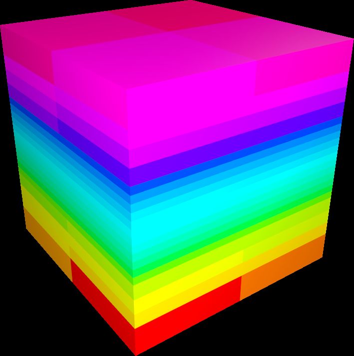

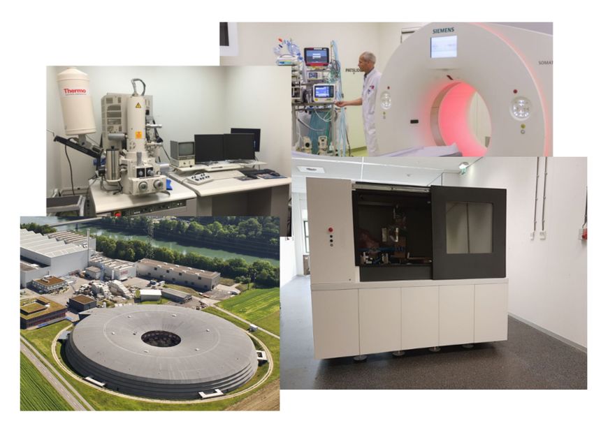
Background

Tomography applications

                          2

Tomography

             3

Reconstruction problem

    • TODO big data sets, typical sizes, different acquisition geometries
    • Distributed 3D volume over many GPUs, minimizing communication

                                                                            4

Communication in tomography

    • Each combination source position and detector pixel defines a ray, in
      the solver each ray is traced through the discretized 3D volume
    • Tomographic reconstruction problem deal with anywhere between
      109 and 1011 rays
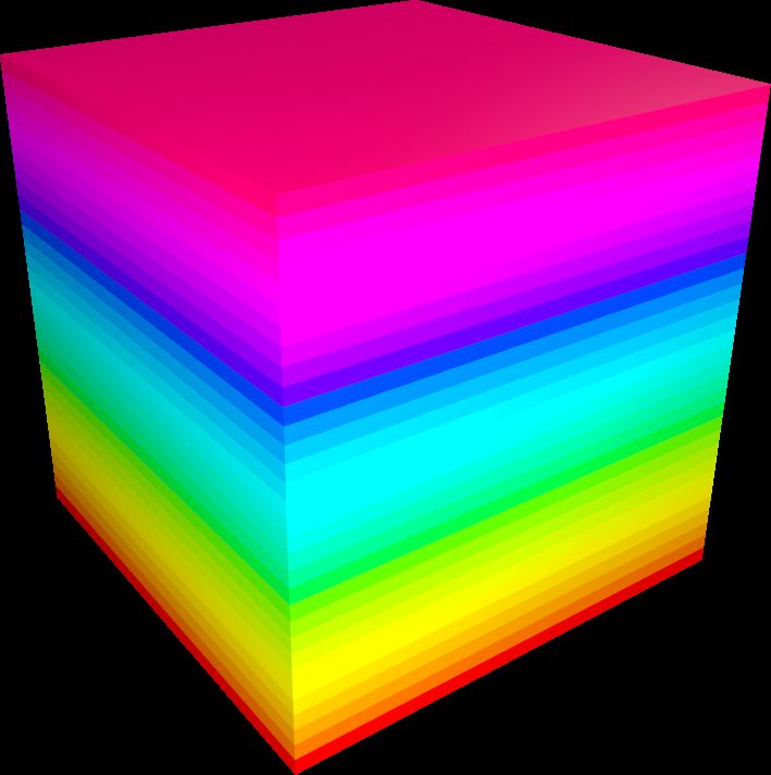
                                                                              5

Partitionings in tomography

    • Partition 3D volume while minimizing the line cut
    • The line cut is the number of additional parts a line crosses
    • Assigning the entire volume to a single GPU is still a partitioning.
      Good for communication, but defeats the purpose.
    • The load of a voxel is the number of rays crossing it. The load of a
      part is the sum over the loads of its voxels.
    • A good partitioning ensures that each part has a similar load.

                                                                             6

Previous work

    Problem (Tomographic partitioning)
   Let V be a cuboid, and G a set of rays through V . Find a p-way
   partitioning of V , that minimizes the total line cut, while ensuring that
   the parts have a roughly equal load.

    • Recursive bisectioning strategy: recursively split V in two,
      somewhere along one of the three axes.
    • It is possible to find the best partitioning of this kind in
      O(p|G| log |G|) time (GRCB algorithm).
    • Communication reduced by between 60% and 90%
    • Each GPU guaranteed to perform the same amount of work

       A geometric partitioning method for distributed tomographic reconstruction.
       JWB, Rob Bisseling, Joost Batenburg. Parallel Computing, 2019.
       doi:10.1016/j.parco.2018.12.007

                                                                                     7

Projection-based partitioning

Shadows

   • Reducing the input size: look at projections instead of rays.

                                                                     8

Shadow overlap

    • Communication volume is proportional to area of the shadow
      overlaps of parts.

                                                                   9

Algorithm sketch

    Subroutine: communicationVolume
    Input: VL , VR , projection set Π
    Output: communication volume Θ

    Θ←0
    for all π ∈ Π do
      shadowL ← convexHull
                   | {z    | {z }(π, corners(VL )))
                         }(project
                       2           1
      shadowR ← convexHull(project(π, corners(VR ))
      Θ ← Θ + area
              | {z }(shadow L ∩ shadowR )
                     |        {z      }
                4             3
    if consider gradient then
       Θ ← Θ + M × area(VL ∩ VR )

                                                      10

Continuous load balance

    • If we have a candidate partitioning, we can efficiently estimate the
      communication volume using the part shadows.
    • Generating candidate partitionings involve finding a projection-based
      estimate for the load. (Number of rays crossing voxels).
    • Estimate by integrating over ray densities for each source point.
      Find c such that:

               Z   c   Z   y2   Z      |Π|
                                    z2 X
                                                        1
                                                                  dz dy dx
                x1     y1       z1                ||~x − ~sk ||22
                                         k=1
                                Z       x2   Z   y2   Z      |Π|
                                                          z2 X
                                                                         1
                            =                                                      dz dy dx .
                                    c        y1       z1           ||~x − ~sk ||22
                                                            k=1

                                                                                                11

Equal load

    • We can reduce the integral to 2D, and then solve numerically:
                  Z   x2   Z   y2 |Π|
                                 X         1              z2 − sk,z
                                                                        
                                                    arctan
                                        ak (x , y )        ak (x , y )
                   x1      y1    k=1                                                 (1)
                                                         z − s 
                                                           1   k,z
                                           − arctan                        dy dx ,
                                                           ak (x , y )
       where                               p
                           ak (x , y ) =       (x − sk,x )2 + (y − sk,y )2 .
    • For certain acquisition geometries, need to consider the cone instead
      instead of the entire cuboid. We reject samples outside cone.
    • Most successful strategy we found so far is an adaption of a
      standard streaming median find algorithm.

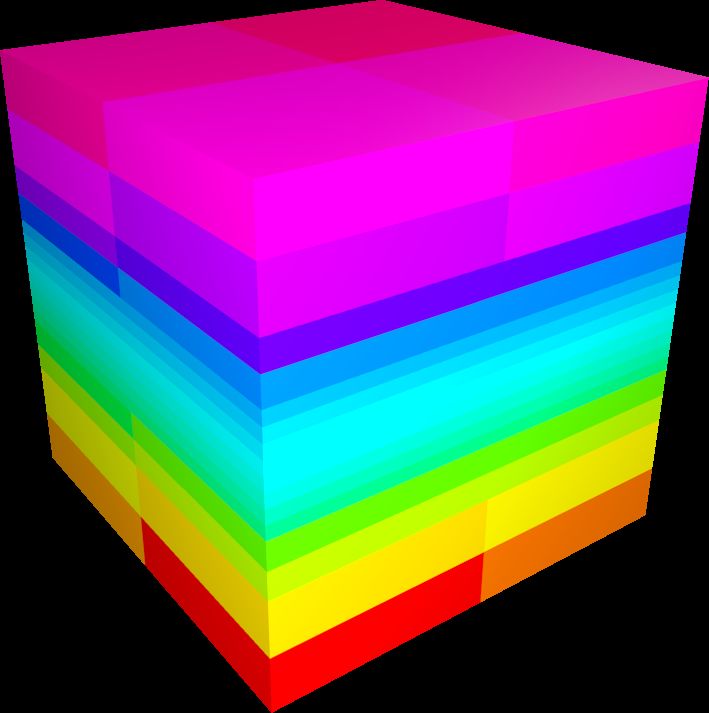
                                                                                           12

Partitioning results

    • Partitioning method: Use continuous load balance to find candidate
      splits in each direction, use shadow characterization of the
      communication volume to choose the best split. Recurse on the
      subvolumes.
                                                                           13

Communication data structures

    • Overlap structures: finding (possibly non-simple, non-convex)
      polygons for each set of contributors.                          14

Overlap algorithm

    Subroutine: FindFaces
    Input: π = {Vs }, πk
    Output: overlay

    overlay ← EmptyArrangement
    for 0 ≤ s < p do
      shadows ← convexHull(project(πk , vertices(Vs )))
      arrangements ← FromFaceTag(shadows , [s])
      merge(overlay, arrangements , concatenate)

    • Subdivision merging algorithms: "find area on map with forests, low
      precipitation, high temperature".
    • We rasterize the resulting faces, and perform aggregrate reads from
      GPU textures containing image data for communication between
      nodes

                                                                            15

Reconstruction times

               200.0

               150.0
       T (s)

               100.0

                           ccbn (Pleiades)
                50.0       ccbw (Pleiades)
                           hcb (Pleiades)
                           ccbn (ASTRA-MPI)
                           ccbw (ASTRA-MPI)
                 0.0
                       8               16         32
                                              p
                                                       16

Conclusion

    • TODO Faster, equal results

                                   17