A Study of Point Laser for Automatic Local Road Condition Assessment: Feasibility, Challenges, and Limitations - UCL Discovery
←
→
Page content transcription
If your browser does not render page correctly, please read the page content below
This article has been accepted for inclusion in a future issue of this journal. Content is final as presented, with the exception of pagination.

            A Study of Point Laser
          for Automatic Local Road
           Condition Assessment:
         Feasibility, Challenges, and
                  Limitations
                                                              Wenda Li
                               Is with the Department of Civil Engineering, University of Birmingham,
                                                   U.K. Email: w.li@bham.ac.uk

                                                        Michael Burrow
                           Is with the Department of Civil Engineering, University of Birmingham, U.K.
                                                Email: m.p.burrow@bham.ac.uk

                                                           Nicole Metje
                           Is with the Department of Civil Engineering, University of Birmingham, U.K.
                                                  Email: n.metje@bham.ac.uk

                                                       Gurmel Ghataora*
                           Is with the Department of Civil Engineering, University of Birmingham, U.K.
                                               Email: g.s.ghataora@bham.ac.uk
                                                                                                                                                                            XXXXXXX

             Abstract—Road condition assessment plays an important role in maintaining the integrity of mature and
             fast-expanding road networks. Such assessments provide invaluable information for local authorities that
             enable them to deliver timely preventative road network maintenance. To enable the best use of scarce
             maintenance resources, it is necessary to assess the condition of the roads periodically. In this article, we
             present the Point Laser (PL) system as an alternative approach for automatic road assessment. Compared
             to current systems, ground penetrating radar and the mobile laser scanning system, the PL system has the
             advantages of low hardware cost, low computational requirements, and fewer environmental restrictions

         Digital Object Identifier 10.1109/MITS.2021.3082505
         Date of current version: 18 June 2021                                                     *Corresponding author.

                                             IEEE INTELLIGENT TRANSPORTATION SYSTEMS MAGAZINE •               2   • MONTH 2021                                1939-1390/21©2021IEEE
Authorized licensed use limited to: University College London. Downloaded on August 23,2021 at 11:21:27 UTC from IEEE Xplore. Restrictions apply.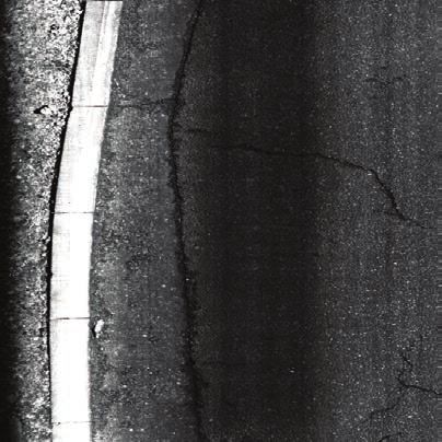
This article has been accepted for inclusion in a future issue of this journal. Content is final as presented, with the exception of pagination.

      in relation to its use. The article first outlines the principle of the PL system including a low-complexity signal pro-
     cessing approach. Afterward, the feasibility, challenges, and limitations of the PL system are discussed based on its
     use in a real environment. A visual-based road survey is used as a ground truth to determine the PL’s performance
     in relation to the requirements of road condition assessment at various levels of road management. The results of
     the comparison demonstrate that the PL system is an ideal candidate for the automatic assessment of the condition
     of local road networks, especially those that require frequent assessment for road asset management.

I
  n most countries, local roads (i.e., urban and rural roads)                                  contrast, MLS is a more mature system and has been used
  constitute by far the largest proportion of the road net-                                    for vehicle-based surveys [4], [9–11]. On the other hand,
  work (typically more than 80%), provide significant so-                                      there are opportunities for the road condition assessment
  cioeconomic benefit, and constitute a significant asset                                      industry to learn from the rapid development of machine/
value to a country. However, due to the combined damag-                                        deep learning, vision systems that have become a critical
ing effects of traffic and the environment, local roads con-                                   component of the autonomous vehicles. Zhang et al. [12]
tinually deteriorate and require periodic maintenance. Not                                     developed a convolutional neural network for road crack-
only does maintenance sustain the value of local roads; it                                     ing detection based on the images collected by a low-cost
also helps to minimize road use costs that are directly re-                                    camera. A more advanced image system shown in Zhang
lated to road condition and thereby helps to ensure socio-                                     et al. [13] can achieve pixel-level accuracy for extracting
economic benefit at minimum user cost [1]. However, local                                      pavement defect to an accuracy of 90%. Accelerometer-
road maintenance is often overlooked in favor of a coun-                                       based approaches are affected by vehicle speed, mass,
try’s high volume, strategic road network. To redress this                                     type, suspension system, and tire pressure [5]. The use
balance there is a need to periodically assess local road                                      of accelerometer-based approaches for the assessment
condition to provide evidence for the need and benefit of                                      of road surface cracking and fretting, the predominant
their maintenance. Due to their vast extent, this should ide-                                  modes of deterioration of local roads, is untried and would
ally be carried out by automated means. However, the au-                                       seem extremely challenging, and therefore research to
tomated assessment of local road condition is challenging                                      date in their use has focused on assessing road roughness
because their predominant modes of deterioration, crack-                                       [5]. The limitations and restrictions of these systems are
ing and fretting (i.e., surface deterioration, which leads to                                  varied. Acoustic/ultrasonic systems are easily disrupted
potholes), are problematic to assess automatically in all                                      by air, gas, and water that restrict their potential applica-
weather conditions at normal traffic speeds. This difficulty                                   tion for high-speed surveying. The signal processing for
is further exacerbated because of the variety of surface                                       MLS is usually highly complex and requires significant
types that can be used to construct local roads. Conse-                                        computational power. Furthermore, the research reported
quently, traditionally the assessment of local road crack-                                     earlier [4], [9–11] has not demonstrated the ability for real-
ing and fretting is normally carried out visually by trained                                   time processing. In addition, the powerful laser beam may
inspectors walking along the road or by using windshield                                       be hazardous to passing pedestrians/animals. The signal
surveys. However, the increasingly faster computing units,                                     processing for MLS is usually with high complexity that
more advanced digital storage devices, and intelligent sig-                                    requires significant computational power, whereas the
nal processing have the potential for both the quantitative                                    works mentioned earlier [4], [9–11] had not demonstrated
and qualitative analysis of local road conditions at traffic                                   the ability of real-time processing. The powerful laser
speeds in real time and at relatively low cost [2].                                            beam may cause hazards to the surrounding pedestrians/
    A variety of vehicle-mounted sensors for automated                                         animals. In comparison, visual systems require suitable
road condition assessment have been investigated, in-                                          levels of road surface illumination; therefore, their use
cluding ground penetrating radar (GPR) [3], mobile laser                                       is constrained during inclement weather, and they often
scanning (MLS) [4], accelerometer [5], and vision system                                       need large amounts of training data, increasing the costs
[6]. These have potential advantages over manual tech-                                         of road surveys. These drawbacks significantly impinge on
nologies, including improved repeatability, reproducibil-                                      their use for extensive local road surveys where the weath-
ity, greater efficiency, and fast development cycles. For                                      er can change rapidly, illumination levels vary, the types
example, previous research on acoustic [7] and ultrasonic                                      of defects vary, and the road surface types vary during the
[8] systems (which transmit the mechanical wave from 50                                        survey.
Hz to 20 MHz) demonstrate the potential for nondestructive                                         Current and future developments of onboard technolo-
road condition assessment with acceptable resolution. In                                       gies for private vehicles include the adoption of both video

                                                 IEEE INTELLIGENT TRANSPORTATION SYSTEMS MAGAZINE •               3   • MONTH 2021
    Authorized licensed use limited to: University College London. Downloaded on August 23,2021 at 11:21:27 UTC from IEEE Xplore. Restrictions apply.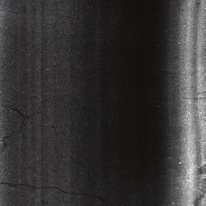
This article has been accepted for inclusion in a future issue of this journal. Content is final as presented, with the exception of pagination.

cameras and inertial (accelerometer)-based equipment.                                        Overview of Point Laser System
While such equipment could be usefully used together with
appropriate processing algorithms to assess road defects,                                    Principle of Point Laser
such as roughness, rutting, and large areas of cracking, for                                 A laser sensor continuously emits a pulse at a near-infra-
the reasons outlined earlier, video and inertial-based sys-                                  red wavelength, and part of the scattered reflected sig-
tems are unsuitable for local roads where the assessment                                     nal is captured by the sensor and digitized. Based on the
of fretting and areas of small cracks is of primary impor-                                   travel time of the light, the relative distances between the
tance. Furthermore, the use of data from private vehicles                                    laser and scanned objects can be calculated from the time
to assess road condition relies on data being recorded on                                    delays between the pulse transmission and return. In
the same section of road by passes of multiple vehicles [5].                                 practice, the laser sensor utilizes optical 2D triangulation
However, rural roads are often very lightly trafficked, and                                  as shown in Figure 1, whereas the angle of the reflected
therefore such an approach would not be feasible.                                            pulse depends on the distance. Unlike most commercial
    In this article, we present an alternative approach for                                  MLS systems, the PL system does not scan the entire road
local road condition assessment that deploys a PL system                                     surface but only the longitudinal direction (i.e., in the di-
that addresses many of the drawbacks of other systems de-                                    rection of travel). As a result, each PL sensor outputs a 2D
scribed earlier. Furthermore, the PL system has the advan-                                   profile of the road surface instead of the 3D point cloud
tage of a relatively low-density of scanning data compared                                   data, which means the down-conversion process is not re-
to the MLS system, thereby reducing computational power                                      quired. This enables much lower computational complex-
requirements, thus facilitating real-time processing. Fur-                                   ity when compared to the 3D MLS point clouds technique
thermore, it costs considerably less than the MLS system                                     or the 2D georeferenced feature (GRF) images [17].
and allows for rapid data update. The PL system has an ex-                                       A road is typically constructed of several layers of mate-
cellent resolution in the longitudinal direction (0.8 mm in                                  rials. Over time, due to the damaging effects of traffic and
this work) and is less hazardous to the surrounding envi-                                    the environment, the road surface loses aggregate particles
ronment. There has been little published work on the PL                                      as the binder ages, causing a consequential loss of adhe-
system. For example, [14] measures the road texture on the                                   sion (this is known as fretting). A PL sensor can detect this
local roads, [15] assesses the road condition at the network                                 loss of the aggregate due to its high resolution. An idealized
level, and [16] uses the root-mean-square (RMS) value to                                     scanning simulation for a PL sensor is shown in Figure 1.
estimate the change in road surface texture. In this work,                                   For a sound road surface, the amplitude and frequency of
a robust and low-complexity signal PL-based processing                                       the reflected laser signal are relatively constant, whereas
methodology has been presented that deals with noise and                                     for a damaged road surface, the reflected signal is of much
estimates road conditions to a resolution suitable for net-                                  greater variation in terms of amplitude and frequency.
work-level analysis. The output is compared with manu-                                       Thus, it is possible to assess the quality of the road sur-
ally inspected data to quantify the similarity. Afterward,                                   face by using information regarding the reflected ampli-
the performance of the PL system is compared to another                                      tude and frequency of the signal. However, in reality, noise
onboard MLS system to demonstrate the advantages and                                         from multiple sources, for example the acceleration from
disadvantages of the proposed PL system for road condition                                   vehicle and the change in the surface texture of the road,
surveys.                                                                                     induce significant interference. For accurate road condi-
                                                                                                                      tion assess, such noise needs to be
                                                                                                                      removed before processing. Details
                                                                                                                      of how this has been achieved in the
             Pulse            Pulse
          Transmitter        Receiver                 Laser Sensor                                                    proposed system are described in
                                                                                                                      the “Preprocessing” section.
                                                               Ideal Scanning                            Road
                                                                  Simulation                            Surface
                                                                                                        Material                System Design
                                                                                                                                The PL system is mounted on an in-
                                                                                                                                service road condition survey ve-
                                                                                                                                hicle (a Ford TDCi model), namely,
                                                                                                                                Highways England’s Road Research
                                                                                                                                Information System 2 (HARRIS2)
                                                                                                                                [15]. The system consists of three
                                                                                                                                main components: sensors for road
                       Good Road Surface                               Damaged Road Surface                                     condition assessment, a system for
                                                                                                                                providing location information, and
FIG 1 An overview of point laser for road condition assessment.                                                                 a central control unit.

                                               IEEE INTELLIGENT TRANSPORTATION SYSTEMS MAGAZINE •               4   • MONTH 2021
  Authorized licensed use limited to: University College London. Downloaded on August 23,2021 at 11:21:27 UTC from IEEE Xplore. Restrictions apply.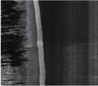
This article has been accepted for inclusion in a future issue of this journal. Content is final as presented, with the exception of pagination.
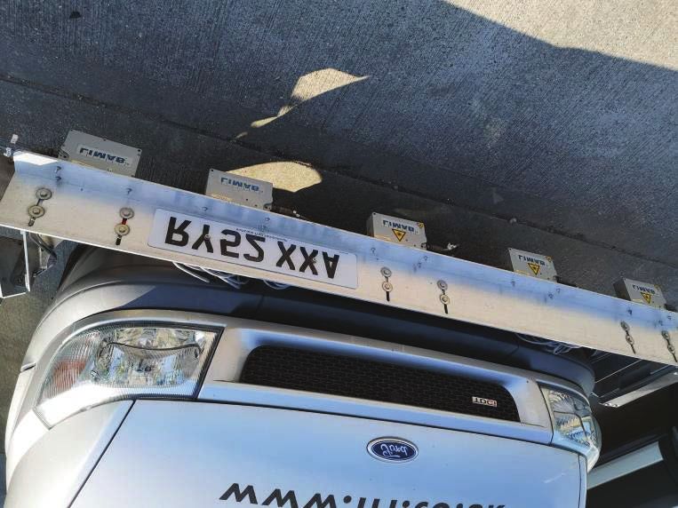
Scanning Sensors
HARRIS2 contains five ProfiCura 2D point lasers [18] de-
signed for operating in the harsh road environment. Each Point Laser
laser is aligned at 90 degrees to the road surface, and the
lasers are distributed horizontally across the vehicle. A
close view of the PL system is shown in Figure 2. HAR-
RIS2 is also equipped with a Laser Crack Measurement
System (LCMS) [19] with high resolution in the transverse
direction that is capable of taking 1,000 transverse profile
measurements per second across a width of approximately
4.2 m. The LCMS collects the 3D laser data from the road
surface and converts it into 2D georeferenced images, and
it is operated simultaneously with the PL system for com-
parison purposes.
Table 1 compares 2D profile data along with 2D
image-driven and 3D MLS point-drive extraction road FIG 2 The point laser system mounted on the HARRIS2.
condition monitoring systems. The PL sensor used in
this work outputs a 2D profile data with the lowest data
dimension compared to the other laser techniques [3], Table 1. Comparison table of laser systems.
[19–21]. Also, a low-complexity histogram analysis [22] 360 Degree
has been used to process the profile data. In compari- Systems Point Laser Onboard MLS MLS [20]
son, converting the 3D MLS point clouds into 2D images
Longitudinal 0.803 mm 4 mm 8 mm
is an effective solution to overcome inconsistency and
Resolution
variance issues in intensity that can occur due to the
shape of road objects. This approach also reduces the Transverse NaN 1 mm 8 mm
Resolution
dimensions of the data and the need to use very robust
deep learning algorithms to analyze the data. In com- Vertical Resolution 0.01 mm 1 mm 8 mm
parison, the 3D point cloud-based systems [20] can im- Categories 2D Profile 2D 3D Point cloud
prove the accuracy of assessing complex types of road data Georeferenced data
defects. However, it is a challenging task to extract from image
the large-volume MLS point clouds especially for un- Signal Processing Histogram Hough Deep learning
evenly distributed point clouds and complex concavo- Method analysis transformation neural network
convex features [17]. Measurement Rate 2k/sec 28k/sec 550k/sec
(max)
Navigation and Orientation System Information Network-level Road markings, Multiple
An important component of automated systems used to as- information road crackings transportation
sess road condition is location referencing. HARRIS2 uses information
a global navigation satellite system (GNSS), which uses a Real-Time Ability Onboard Offline No demonstration
GPS signal to provide the location information in the form processing processing
of an Ordnance Survey grid reference (OSGR) (OSGR is a
grid references system used in the United Kingdom). The
positioning accuracy of this system is affected by mul- Central Control Unit
tipath propagation issues (for example, tunnels, build- HARRIS2 also contains a central control unit (a comput-
ings, and trees). To eliminate such effects and bypass the er server), a highly integrated control system designed
limitation of GPS signal, an inertial measurement unit to control all onboard sensors (e.g., laser system, MLS),
(IMU) is used to provide the instant velocity, position, and synchronize the data from each system with a time stamp,
attitude measurements. The IMU provides continuous and store the location information from the GNSS system.
positioning information in the case of GNSS malfunction. Further information about the HARRIS2 central control
In addition, the IMU contains three accelerometers and unit can be found in [15].
three gyroscopes, which can also be used for acceleration
and angular measurements. The resulting overall local- Signal Processing of Point Laser
ization accuracy is approximately 1 cm horizontally and This section presents the signal processing for the pro-
2 cm vertically with respect to local GNSS-reference sta- posed PL system that is used to 1) remove noise and 2) ana-
tions [17]. lyze the processed signal to estimate road condition. The
IEEE INTELLIGENT TRANSPORTATION SYSTEMS MAGAZINE • 5 • MONTH 2021
Authorized licensed use limited to: University College London. Downloaded on August 23,2021 at 11:21:27 UTC from IEEE Xplore. Restrictions apply.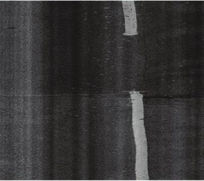
This article has been accepted for inclusion in a future issue of this journal. Content is final as presented, with the exception of pagination.
structure of the developed signal processing is shown in where y (t) represents the collected data points, l n is the
Figure 3. window length, c i = 1/ (l n + 1) is the weighting factor, and
w is a constant. Data points above the threshold are con-
Preprocessing sidered to be erroneous [e.g., the red line in Figure 4(a)].
It was observed that several sources of noise can affect The second step replaces erroneous data points with the
significantly the PL data, and such noise therefore needed mean value of authentic adjacent data points. In the ex-
to be filtered at the preprocessing stage. To illustrate this, ample given in Figure 4(a), the resulting data points are
an example of 50-meter raw data points is provided in shown in Figure 4(b).
Figure 4(a).
Vehicle Dynamic
Sensor Noise Another major source of interference is from vehicle
Sensor noise is a result of the PL sensor recording an vibrations, which are particularly prevalent during
erroneous data point due to the internal clock issues acceleration and deceleration. Since the laser sensor
(signal source inside PL sensor) providing an incor- measures the relative distance to the road surface, a
rectly measured time of f light between the outward change in vehicle height may affect the measurement
and ref lected laser pulses. By analyzing the entire of road defects. In this work, the vehicle dynamic is-
data set from a survey, the erroneous data point typi- sue was regarded as a baseline correction problem
cally accounts for approximately 0.5% of the data. since the motion introduces components that have sig-
Since the longitudinal resolution of the PL sensor nificantly greater f luctuations in both magnitude and
is 0.803 mm, this means around six erroneous data wavelength when compared to those resulting from
points per meter. These erroneous data points are of both the road texture and the defects. The MAM algo-
much higher amplitude [as shown in Figure 4(a)] and rithm described in (1) was used again for the baseline
can cause significant interference for the later histo- estimation (albeit with a different window length). Ac-
gram analysis. cordingly, the resulting corrected data points yt (t) are
In this work, a two-step algorithm was applied to re- calculated as
move the erroneous data points while not affecting the
other authentic data points. First, an adaptive threshold yt (t) = y (t) - y V (t) ,(2)
T (t) based on a moving average of minima (MAM) method
[23] was used to identify the erroneous data points. T (t) is where y V (t) is the estimated baseline. The result of base-
calculated as follows: line correction is shown in Figure 4(c), from which it
can be seen that the major component due to the vehicle
1l
2 n dynamic has been successfully corrected. For example, the
T (t) = / c i y (t + i) + w ,(1) troughs (e.g., near 10 and 40 meters) can be easily observed
i = - 1 ln following the baseline correction.
2
Adaptive Baseline Local Area
Threshold Estimation (Monitoring)
Raw Data Replace Remove
Pixel RTI Histogram Parameter
From Laser Erroneous Vehicle
Calculation Feature Calculation
Sensor Data Points Dynamic
Histogram Global Area
Preprocessing (Road
Analysis
Texture)
FIG 3 A block diagram of signal processing for point laser.
IEEE INTELLIGENT TRANSPORTATION SYSTEMS MAGAZINE • 6 • MONTH 2021
Authorized licensed use limited to: University College London. Downloaded on August 23,2021 at 11:21:27 UTC from IEEE Xplore. Restrictions apply.
This article has been accepted for inclusion in a future issue of this journal. Content is final as presented, with the exception of pagination.
400 200
Measurement (mm)
Measurement (mm)
300 150
200 100
100 50
0 0
0 10 20 30 40 50 0 10 20 30 40 50
Distance (m) Distance (m)
(a) (b)
30
Measurement (mm)
20
10
0
–10
–20
0 10 20 30 40 50
Distance (m)
(c)
4 4
Measurement (mm)
Measurement (mm)
2 2
0 0
–2 –2
–4 –4
–6 –6
0 0.5 1 1.5 2 0 0.5 1 1.5 2
Distance (m) Distance (m)
(d) (e)
0.6 0.6
Local Local
Frequency of Occurrence
Frequency of Occurrence
Global Global
0.4 0.4
0.2 0.2
0 0
0 1 2 3 0 1 2 3
RTI Value RTI Value
(f) (g)
FIG 4 A demonstration of the signal processing for a PL system: (a) raw data points (the red line is adaptive threshold); (b) after sensor noise removal;
(c) after baseline correction (the red part is road surface containing fretting; the green part is a sound road surface); (d) and (e) measurements of two
types of road texture; (f) histogram analysis of fretting road surface; and (g) histogram analysis of smooth road surface.
IEEE INTELLIGENT TRANSPORTATION SYSTEMS MAGAZINE • 7 • MONTH 2021
Authorized licensed use limited to: University College London. Downloaded on August 23,2021 at 11:21:27 UTC from IEEE Xplore. Restrictions apply.
This article has been accepted for inclusion in a future issue of this journal. Content is final as presented, with the exception of pagination.

Road Condition Estimation                                                                    similarity of the vectors. Two parameters were chosen to
Another issue that needs to be considered is the changes in                                  this end:
road surface texture that are likely to be encountered by a                                  ■■ Mean-square-error (MSE). MSE represents the differ-
survey vehicle during a survey. Different road textures can                                     ence between the RTI distribution of the local and sur-
have different sizes of surface aggregate, and as a result,                                     rounding global lengths. A low MSE value occurs if the
this can cause issues in the measurement of fretting at the                                     distributions of local and global RTI values are similar,
point when the vehicle traverses two roads with different                                       and thus there is a low amount of fretting in the local
surface textures. Examples of two different road textures                                       length. MSE is calculated as MSE = 1 n R ni = 0 h g - h l ,          i   i

are shown in Figure 4(d) and (e).                                                               where h g and h l are the histogram features from glob-
                                                                                                                 i           i

                                                                                                al and local area.
Road Texture Index Calculation                                                               ■■ Correlation-coefficient (R). R is a measure of the simi-
The Root Texture Index (RTI) was adopted as a measure of                                        larity between the frequency distribution of the RTI
road texture as discussed in our previous work [22], [24].                                      values of the local length and that of the global length.
RTI evaluates the changes in road surface measurement                                           Low R values indicate that the local RTI distribution
for a given segmentation with respect to the RMS value.                                         is significantly different compared to the global RTI
The ith RTi value is calculated as                                                              distribution, and therefore the local length of road
                                                                                                contains large amounts of fretting. R is calculated as
                  RTI i =         1 / n y (k) 2 ,(3)                                            R = R ni = 0 h g h l nv h v h , where v represents the stan-
                                  ns k = 1 s                                                                         i   i       g    l

                                                                                                dard deviation.
where n s is the number of data points per segmentation.                                        The efficacy of these processes is discussed in the next
                                                                                             section.
Global and Local Area
In this work, the concept of the global area (i.e., an esti-                                 Observations and Discussions
mate the type of road texture over a relatively long distance                                In this section, we discuss the detection performance of
as a reference) and the local area (i.e., the scanning area)                                 the system outlined earlier, using data collected from a
is used [22]. The concept assumes that the road texture                                      number of road surveys. Three challenges are outlined to-
remains unchanged over the long distance (global area)                                       gether with their possible solutions. Limitations are also
when compared to the part of road being assessed (i.e., the                                  discussed to present the boundaries of using the PL system
local area). By doing so, the system can analyze the types                                   for road condition surveys.
of road texture without prior knowledge of the texture fea-
tures. The relationship between the number of data points                                    Feasibility
in global area n g , the local area n l , and the segmentation                               The feasibility of the PL system is demonstrated by compar-
length n s follows n g 2 n l & n s .                                                         ing data collected from four roads near Crowthorne, United
    As a result, the number of RTI values in a global area                                   Kingdom, surveyed by HARRIS2 with the Detailed Visual
is greater than that in a local area, and, consequently, fre-                                Inspection (DVI) [25] of the roads carried out by trained
quency histograms of local and global RTI values are com-                                    surveyors. The DVI survey classifies road surface fretting
pared to assess the condition of the local area compared to                                  in terms of high (H), moderate (M), and low (L) levels. A
the global area. Here, two examples of histogram analysis                                    brief description of the data set is provided in Table 2.
are provided based on the data points in Figure 4(c). The                                        The MSE value against the R value for each road is plot-
section from 5 m to 10 m shows an area of road surface                                       ted in Figure 5 to visualize the algorithm’s output. Each
that has significant fretting (the red part) whereas the sec-                                point represents the PL measurement over a 5 m distance.
tion from 20 m to 25 m is a sound road surface (the green                                    Sound road surfaces should have small MSE value (i.e.,
part). The output histograms are provided in Figure 4(f)                                     close to 0) and a high R value (i.e., close to 1), whereas dam-
and (g), respectively. As can be seen, the histogram of the                                  aged road surface will have a high MSE and a low R value.
sound road surface has a similar distribution to that of the                                 In other words, in Figure 5, data points in top left corner
global area, whereas the fretted road surface shows more                                     represent road sections with low amounts of fretting area,
variance.                                                                                    and those in bottom right corner represent road sections
                                                                                             with a high amount of fretting. Figure 5 presents the aver-
Parameter Calculation                                                                        age condition of each road. For example, the majority of
The final stage is to generate meaningful parameters that                                    sections of road one are in generally good condition with
can present the difference between histograms of a fretted                                   most data points concentrated in the top left corner. On the
and sound road surface meaningfully. Histogram features                                      other hand, the measured sections in road four are scat-
can be considered to be vectors; thus, the problem can                                       tered across the bottom right corner, suggesting the road
be considered to be one of understanding the difference/                                     is in poor condition. In contrast, roads two and three have

                                               IEEE INTELLIGENT TRANSPORTATION SYSTEMS MAGAZINE •               8    • MONTH 2021
  Authorized licensed use limited to: University College London. Downloaded on August 23,2021 at 11:21:27 UTC from IEEE Xplore. Restrictions apply.
This article has been accepted for inclusion in a future issue of this journal. Content is final as presented, with the exception of pagination.

more points distributed among the middle area, indicat-                                          and correspond to their actual road condition. In compari-
ing that the road sections are in moderate condition. By in-                                     son, the majority of MSE values from road four are between
spection, these results match the DVI data shown in Table                                        0.03 and 0.04, and most R values are less than 0.90, indicat-
2. There are also some anomalies, for example, the point                                         ing a damaged road section. This finding is verified by the
(MSE = 0.06 and R = 0) in the right bottom of Figure 5(c).                                       actual condition of the road given in Table 2.
However, the number of anomalies is very small, and they
do not affect significantly the assessment of the average
condition of the entire road. Even in roads three and four,
there are a number of sections with low MSE and high R                                              Table 2. Details of the road survey.
values.
                                                                                                   Road          Description           Length       Class                Fretting Level
   The MSE and R values shown in Figure 5 are presented
in Figures 6 and 7 in the form of histograms of the nor-                                           One           Byron Drive           0.421        Secondary road       L
malized frequency of occurrence. These histograms show                                             Two           Duke’s Ride           0.480        B road               L/M
clearly trends in condition for each road. The majority of
                                                                                                   Three         Wokingham             0.711        A road               M
MSE values for roads one and two lie in the range between
                                                                                                                 Road
0.01 and 0.02 with R values between 0.99 and 0.97. This
                                                                                                   Four          Hanworth Road         1.337        Secondary road       H
suggests that both roads are on the whole in good condition

              1                                                                                        1

            0.8                                                                                     0.8

            0.6                                                                                     0.6

            0.4                                                                                     0.4
       R

                                                                                              R

            0.2                                                                                     0.2

              0                                                                                        0

                  0        0.01       0.02       0.03  0.04             0.05       0.06                    0      0.01       0.02        0.03  0.04            0.05      0.06
                                                  MSE                                                                                     MSE
                                                   (a)                                                                                     (b)

              1                                                                                        1

            0.8                                                                                     0.8

            0.6                                                                                     0.6

            0.4                                                                                     0.4
       R

                                                                                              R

            0.2                                                                                     0.2

              0                                                                                        0

                  0        0.01       0.02       0.03  0.04             0.05       0.06                    0      0.01       0.02        0.03  0.04            0.05      0.06
                                                  MSE                                                                                     MSE
                                                   (c)                                                                                     (d)

FIG 5 An MSE and R plot for each road survey: (a) road one, (b) road two, (c) road three, and (d) road four.

                                                   IEEE INTELLIGENT TRANSPORTATION SYSTEMS MAGAZINE •               9   • MONTH 2021
  Authorized licensed use limited to: University College London. Downloaded on August 23,2021 at 11:21:27 UTC from IEEE Xplore. Restrictions apply.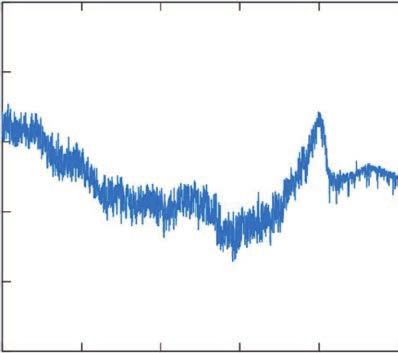
This article has been accepted for inclusion in a future issue of this journal. Content is final as presented, with the exception of pagination.

   Road surveys can be considered to support three levels                                      tentially affect the system’s performance. Four different
of road asset management decision making, namely, stra-                                        types of interference are shown in Figure 9 (the sensor
tegic planning, tactical programming, and operations [26].                                     noise has been removed) varying from a few millimeters to
The data requirements to support each level of decision                                        more than hundred meters in extent and with a variety of
making are different and can be defined according to the                                       magnitudes. For example, data points in Figure 9(a) show
World Bank’s information quality level (IQL) approach [27].                                    a saturated and a constant gap spanning over one meter,
A paired difference test [28] was used to further compare                                      whereas in Figure 9(b) a deep trough of more 50 mm in
statistically the results of the PL system and the DVI meth-                                   depth and 0.1 m in width is apparent at a distance of 0.4
odology for each of the three levels of management. Figure                                     m. In comparison, the apparent anomalies in Figure 9(c)
8 provides the results of strategic planning (500 m), tacti-                                   and (d) are similar to the road measurements in terms of
cal programming (60 m), and operations (20 m). The PL                                          the magnitude and variation, but with a unique periodicity.
system and DVI show similar results for all three levels of                                        The cause for these anomalies varies. Sensor error can
road management. In particular, the similarity is highest                                      explain the measurements in Figure 9(a) and (b) as they
when the data are considered over a 500-m length of road.                                      are of constant amplitude for a period of time, which should
Data to this level of detail are at IQL 3/4 and are suitable                                   not be a case when scanning a road section. For Figure 9(c)
for strategic road asset management decision making [22].                                      and (d), small objects on the road surface may be the rea-
This means the current approach is sufficient for strate-                                      son for those measurements, for example, when the scan
gic, or network-level, road condition analysis. Accordingly,                                   is over a manhole cover or a road marking. Undoubtedly,
this data would be useful to support inspection required                                       these abnormal measurements will affect the RTI calcula-
to determine periodical maintenance and infrastructure                                         tion and the histogram analysis. In the “Feasibility” sec-
construction planning.                                                                         tion, we have demonstrated that with the current setup, the
                                                                                               system output can achieve the requirement of IQL 3/4 for
Challenges                                                                                     network-level analysis. But to achieve a higher level in IQL
                                                                                               1/2, these irregular measurements need to be removed.
Unexpected Measurements                                                                            Anomalies such as those in Figure 9(a) and (b) are easy
Apart from the interference described in the “Preprocess-                                      to detect, as they have very different magnitudes when
ing” section, there are a number of issues that may po-                                        compared to the regular road surface. Algorithms such as
                                                                                               those proposed by [29] could be suitable to identify such
                                                                                               anomalies. The challenge is more complicated for the data
         0.4                                                                                   points in Figure 9(c) and (d), as they may appear more
                                                                 Road One                      frequently. Their detection and removal require training
         0.3                                                     Road Two                      a classifier with a data set labeled as “normal” and “ab-
                                                                 Road Three
                                                                 Road Four                     normal” so that the system can separate the normal and
   (%)

         0.2
                                                                                               abnormal measurements.
         0.1
                                                                                               Road Surface Texture
          0                                                                                    Another challenge is the effect of the change of road tex-
                   01

                    5
                   02

                    5
                   03

                     5
                   04

                     5
                   05

                     5

                                                                                               ture, which can occur during a road condition survey.
                  01

                  02

                  03

                  04

                  05
               0.

                0.

                0.

                0.

                0.
                0.

               0.

               0.

               0.

               0.

                                       MSE Value                                               An example of measurements on two road textures using
                                                                                               an MLS and PL sensors is shown in Figure 10. As can be
FIG 6 A histogram on MSE values from four road surveys.                                        seen, the two types of road texture are clearly distinguish-
                                                                                               able in the 2D image from the MLS with different inten-
                                                                                               sity. In comparison, the difference between two textures
         0.8                                                                                   is not as apparent in the PL measurement, but it still can
                                                                 Road One                      be observed that the data points from road texture A con-
         0.6                                                     Road Two
                                                                 Road Three                    tain more fluctuations than for texture B. Despite the use
                                                                 Road Four                     of the local and global concept described earlier to negate
   (%)

         0.4
                                                                                               the need to determine prior to the survey the type of road
         0.2                                                                                   texture, a larger window than that used for the earlier
                                                                                               analysis is required to show the changes in texture. This
          0
                0.99 0.97 0.95 0.93 0.9 0.85 0.8 0.7 0.6 0.5                                   potentially reduces the accuracy of the output as road de-
                                    R Value                                                    fects vary in size depending on the road texture, while the
                                                                                               inaccurate texture estimation reduces the number of road
FIG 7 A histogram on R values from four road surveys.                                          defects detected.

                                                IEEE INTELLIGENT TRANSPORTATION SYSTEMS MAGAZINE •               10   • MONTH 2021
  Authorized licensed use limited to: University College London. Downloaded on August 23,2021 at 11:21:27 UTC from IEEE Xplore. Restrictions apply.
This article has been accepted for inclusion in a future issue of this journal. Content is final as presented, with the exception of pagination.
The low dimension of data points in a PL survey restricts Improvements can be made to both the software and
the estimation of road texture. A sliding window could help hardware to better account for the effects of vehicle dy-
to improve the sensitivity by generating more estimations namics. From the software side, filters with high-res-
over a given area. However, the global area remains a net- olution spectra that are able to process multivariate can
work-level method as it contains a large number of data provide better performance in baseline correction [30]. But
points that are insensitive to a sudden change and enables the application of such filters can significantly increase
changes in road texture to be considered automatically. the processing time and the choice of appropriate filter
On the other hand, the analysis of very small sections of parameters is critical. On the hardware side, the onboard
the road surface can significantly increase the accuracy of IMU provides the inertial information about the vehicle
texture measurement by examining the characteristics of movement. Real-time vehicle dynamics can be calculated
each data point. Such an approach will require significant by using this information, allowing their effect to be re-
additional computational power due to the larger number moved from the PL measurement with a high degree of
of data points that need to be assessed. Thus, the tradeoff confidence.
between the computational power and accuracy required
to measure texture needs to be carefully considered and Limitations
assessed according to the IQL required. Since the PL sensor scans only in the longitudinal direc-
tion, it has a number of limitations when compared to an
Imperfect Vehicle Dynamic Cancellation MLS system. Based on the analysis of the data obtained
As described in the “Preprocessing” section, an MAM filter from the field trial, it was observed that several road
was used for simple and low-complexity baseline correc- defects are hard to identify by the PL system because
tion. However, the varied dynamic motions of the vehicle their shape or location are not within the scanning
mean a single MAM filter cannot accurately remove all of area. Also, low-level road surface associated features
the dynamic components, and as a result, those compo- (when compared to 3D point cloud data) are apparent
nents that are not removed can strongly affect the histo- in the PL measured data that are problematic for defect
gram analysis. classification.
0.25 0.25 0.25
1 1 1
0.2 0.2 0.2
2 2 2
Category
Category
Category
0.15 0.15 0.15
3 3 3
0.1 0.1 0.1
4 4 4
0.05 0.05 0.05
5 5 5
0 0 0
One Two Three Four One Two Three Four One Two Three Four
Road Road Road
(a) (b) (c)
0.25 0.25 0.25
1 1 1
0.2 0.2 0.2
2 2 2
Category
Category
Category
0.15 0.15 0.15
3 3 3
0.1 0.1 0.1
4 4 4
0.05 0.05 0.05
5 5 5
0 0 0
One Two Three Four One Two Three Four One Two Three Four
Road Road Road
(d) (e) (f)
FIG 8 A comparison of the category result for the management function of planning (500 m) (a) DVI and (b) point laser system; programming (60 m), (c)
DVI and (d) point laser system; and preparation (20 m), (e) DVI and (f) point laser system.
IEEE INTELLIGENT TRANSPORTATION SYSTEMS MAGAZINE • 11 • MONTH 2021
Authorized licensed use limited to: University College London. Downloaded on August 23,2021 at 11:21:27 UTC from IEEE Xplore. Restrictions apply.This article has been accepted for inclusion in a future issue of this journal. Content is final as presented, with the exception of pagination.
Limited Road Information capable of measuring only the surface of the road under-
Road cracking is a common type of defect that occurs on neath the vehicle. A potential solution to the measure-
local roads with asphalt surfacings. Therefore, for a com- ment of both longitudinal cracking and edge wear is to
prehensive condition survey cracking needs to be detected employ sensors at an angle to the road surface so that the
since unchecked cracking can lead to the formation of pot- coverage can extend outside the vehicle. Also, PL sensors
holes and eventual road failure. Road surface cracking can could be mounted away from the vehicle, on a retractable
span both the transverse and longitudinal directions [31]. arm, for example, allowing a greater area to be covered.
As shown in Figure 11, cracking in the transverse direc- These additional PL sensors, however, will increase the
tion can be relatively easily detected by the advocated PL cost of system hardware, and more data points need to be
system. However, cracking in the longitudinal direction is processed.
less likely to be detected by the narrow laser beam.
Another significant defect that occurs on local roads Low-Level Features for Classification
is edge deterioration, which results from a lack of sup- In comparison to the features determined by an MLS system
port and poorly draining shoulder material. This issue (3D point cloud data), the 2D PL system provides fewer (lower-
can soon worsen if the road edge is not repaired in a level) features. Although the PL system can detect road defects
timely fashion. Since edge deterioration is wider than based on the variation in their depth, a single PL cannot assess
road cracking, it should be easily captured by a PL sen- on its own the width or shape of a road defect. For example,
sor, provided that the sensor aligns with the edge of the in Figure 11, cracking in the transverse direction has been
road. However, for the system proposed herein the PL is scanned only a few times, which makes it difficult to assess
120
300
Measurement (mm)
Measurement (mm)
100
200
80
100
60
0
0 5 10 15 0 0.2 0.4 0.6 0.8 1
Distance (m) Distance (m)
(a) (b)
120 140
Measurement (mm)
Measurement (mm)
100
120
80
100
60
80
0 0.5 1 1.5 0 0.5 1 1.5
Distance (m) Distance (m)
(c) (d)
FIG 9 (a)–(d) Examples of different types of abnormal measurements from point laser sensor.
IEEE INTELLIGENT TRANSPORTATION SYSTEMS MAGAZINE • 12 • MONTH 2021
Authorized licensed use limited to: University College London. Downloaded on August 23,2021 at 11:21:27 UTC from IEEE Xplore. Restrictions apply.This article has been accepted for inclusion in a future issue of this journal. Content is final as presented, with the exception of pagination.
the true extent of transverse cracking. This restricts the use global length is 100 m (124,533 data points). Accordingly,
of the PL system, reduces its ability to detect certain types of while the presence of the pothole would influence the his-
defects, and reduces the accuracy of defect classification com- togram analysis described earlier and would probably re-
pared to an MLS-based system. This could be improved by fus- sult in local area of road surface being shown (correctly) to
ing data from more than one PL allied to the use of intelligent contain fretting, the analysis would not be able to identify
algorithms that can infer and extrapolate features from data the individual pothole causing the high degree of fretting.
provided. One possible solution is to use a moving window with vari-
In addition, the local-global principle requires fine- able size. For example, in our previous work [32], a peak
tuning if it is to be used to identify individual small defects, detection approach was used, but it was of much greater
such as potholes. The longitudinal resolution of the PL sen- computational complexity and required greater computa-
sor is 0.803 mm (see Table 1). Therefore, a pothole with a tional effort due to the wavelet transform process. Addi-
diameter of 30 cm would result in approximately 374 data tionally, fusing data from multiple PL sensors will improve
points. This is a relatively small number when compared the feature diversity detectability of the suggested system
with a local length of 10 m (12,453 data points) and the by using the data from different scanning path.
Conclusions
Texture A
This article discussed the use of a PL system for the auto-
Change mated analysis of local road condition at moving traffic
Point speeds. A histogram analysis has been used to process
the scanning data from a PL system with the local-global
concept. The experimental results indicate that the PL
Texture B
system has the capability of satisfactorily assessing local
road condition to IQL 3/4, which is required for strate-
(a) gic road asset management. However, several challenges
180
were observed from the analysis of the field data, includ-
ing the presence of unexpected measurements, issues
Measurement (mm)
170 Texture A Texture B associated with the change in road texture during a road
160 survey, and the effects of vehicle dynamics. A number
of corresponding solutions were proposed with respect
150
Change to efficiency to identify noise and the use of the IMU to
140 Point counteract the effects of vehicle dynamics on the record-
130 ed PL data. It is recognized that the proposed PL system
0 1 2 3 4 5 6 7 8 9 10 is unable to detect a number of features that could be
Distance (m)
provided by a MLS system, thus limiting its application
(b)
to the types of defects that can be detected and the IQL of
those defects it is able to detect. It is recognized therefore
FIG 10 Data comparison between (a) a laser image from onboard MLS
system and (b) the texture data from point laser system. that while the proposed PL system is able to assess road
surface condition to a sufficient level to support strategic
level road asset management, further enhancements are
Scanning Path of Point Laser required to improve its detection performance in terms
of accuracy and coverage and thereby enable road condi-
tion to be assessed to higher IQLs. These enhancements
include fusing data from a number PLs allied to more
intelligent data processing algorithms.
Acknowledgments
Direction
The authors are grateful for the financial support provided
by the U.K. Technology Strategy Board through Innovate.
The practical contribution of the Department of Civil En-
gineering at the University of Birmingham, U.K., is appre-
Cracking in Cracking in ciated. We also gratefully acknowledge the support from
Transverse Direction Transverse Direction Highways Surveyors Ltd and the Transport Research Labo-
ratory (TRL) Ltd which provided road condition data cap-
FIG11 A demonstration of a point laser scanning path. tured using HARRIS2.
IEEE INTELLIGENT TRANSPORTATION SYSTEMS MAGAZINE • 13 • MONTH 2021
Authorized licensed use limited to: University College London. Downloaded on August 23,2021 at 11:21:27 UTC from IEEE Xplore. Restrictions apply.This article has been accepted for inclusion in a future issue of this journal. Content is final as presented, with the exception of pagination.
[3] M. E. Torbaghan, W. Li, N. Metje, M. Burrow, D. N. Chapman, and C.
About the Authors D. Rogers, “Automated detection of cracks in roads using ground pen-
Wenda Li (w.li@bham.ac.uk) earned etrating radar,” J. Appl. Geophys., vol. 179, p. 104,118, Aug. 2020. doi:
10.1016/j.jappgeo.2020.104118.
his Ph.D. degree in the Department of [4] S. C. Radopoulou and I. Brilakis, “Improving road asset condition
Electrical and Electronic Engineering monitoring,” Transport. Res. Proc., vol. 14, pp. 3004–3012, 2016. [On-
line]. Available: https://www.sciencedirect.com/science/article/pii/
at the University of Bristol. He is cur- S2352146516304434, doi: 10.1016/j.trpro.2016.05.436.
rently an honorary research fellow in [5] S. Sattar, S. Li, and M. Chapman, “Road surface monitoring using
smartphone sensors: A review,” Sensors, vol. 18, no. 11, p. 3845, 2018.
the Department of Civil Engineering, doi: 10.3390/s18113845.
University of Birmingham, Birming- [6] C. Koch, K. Georgieva, V. Kasireddy, B. Akinci, and P. Fieguth, “A re-
view on computer vision based defect detection and condition assess-
ham, B15 2TT, United Kingdom. His research interests ment of concrete and asphalt civil infrastructure,” Adv. Eng. Inf., vol.
include signal processing for radar-based applications, in- 29, no. 2, pp. 196–210, 2015. doi: 10.1016/j.aei.2015.01.008.
[7] S. Paje, M. Bueno, F. Terán, U. Viñuela, and J. Luong, “Assessment of
cluding passive Wi-Fi radar and penetrate ground radar. asphalt concrete acoustic performance in urban streets,” J. Acoustical
He is also interested in sensory signal analysis for autono- Soc. Amer., vol. 123, no. 3, pp. 1439–1445, 2008. doi: 10.1121/1.2828068.
[8] Y. Taniguchi, K. Nishii, and H. Hisamatsu, “Evaluation of a bicycle-
mous vehicle and automatic road network assessment. mounted ultrasonic distance sensor for monitoring road surface con-
dition,” in Proc. 7th Int. Conf. Comput. Intell., Commun. Syst. Netw.
(CICSyN), 2015, pp. 31–34. doi: 10.1109/CICSyN.2015.16.
Michael Burrow (m.p.burrow@bham [9] D. Barber, J. Mills, and S. Smith-Voysey, “Geometric validation of a
.ac.uk) earned his Ph.D. degree in road ground-based mobile laser scanning system,” ISPRS J. Photogram.
Remote Sens., vol. 63, no. 1, pp. 128–141, 2008. doi: 10.1016/j.is-
asset management from the University prsjprs.2007.07.005.
of Birmingham, Birmingham, B15 2TT, [10] H. Guan, J. Li, Y. Yu, M. Chapman, and C. Wang, “Automated road in-
formation extraction from mobile laser scanning data,” IEEE Trans.
United Kingdom. He is a senior lecturer Intell. Transp. Syst., vol. 16, no. 1, pp. 194–205, 2015. doi: 10.1109/
in the School of Engineering, Universi- TITS.2014.2328589.
[11] M. Lehtomäki et al., “Object classification and recognition from mo-
ty of Birmingham. His research inter- bile laser scanning point clouds in a road environment,” IEEE Trans.
ests include infrastructure asset management. Geosci. Remote Sens., vol. 54, no. 2, pp. 1226–1239, 2016. doi: 10.1109/
TGRS.2015.2476502.
[12] L. Zhang, F. Yang, Y. D. Zhang, and Y. J. Zhu, “Road crack detection us-
Nicole Metje (n.metje@bham.ac.uk) ing deep convolutional neural network,” in Proc. 2016 IEEE Int. Conf.
Image Process. (ICIP), pp. 3708–3712. doi: 10.1109/ICIP.2016.7533052.
earned her Ph.D. degree from the [13] A. Zhang et al., “Automated pixel-level pavement crack detection on
University of Birmingham in 2001. 3d asphalt surfaces using a deep-learning network,” Comput.-Aided
Civil Infrastruct. Eng., vol. 32, no. 10, pp. 805–819, 2017. doi: 10.1111/
She is a professor of infrastructure mice.12297.
monitoring at the University of Bir- [14] H. Viner, P. Abbott, A. Dunford, N. Dhillon, L. Parsley, and C. Read,
“Surface texture measurement on local roads,” Transport Research
mingham, Birmingham, B15 2TT, Lab., Wokingham, Project Report PPR148, 2006.
United Kingdom. Her research focuses [15] A. Wright, N. Dhillon, S. McRobbie, and C. Christie, “New methods for
network level automated assessment of surface condition in the UK,”
on detection of buried infrastructure and the development in Proc. 7th Symp. Pavement Surface Characteristics, Norfolk, VA, Sept.
and use of sensing technologies to see through the ground 19–22, 2012.
[16] S. McRobbie, A. Wright, J. Iaquinta, P. Scott, C. Christie, and D. James,
and/or assess the condition of infrastructure assets. “Developing new methods for the automatic measurement of raveling
at traffic-speed,” in Proc. 11th Int. Conf. Asphalt Pavements, Nagoya,
2010.
Gurmel Ghataora (g.s.ghataora@bham [17] L. Ma, Y. Li, J. Li, C. Wang, R. Wang, and M. Chapman, “Mobile laser
.ac.uk) earned his Ph.D. degree. in civil scanned point-clouds for road object detection and extraction: A review,”
Remote Sens., vol. 10, no. 10, pp. 1531, 2018. doi: 10.3390/rs10101531.
engineering from the University of [18] “ProfiCura sensor family – 2D laser sensors for profile measurements.”
Wales, Cardiff. He is currently a senior LIMAB. Accessed: May 1, 2021. [Online]. Available: http://www.limab
.com/products/proficura-2d-2/
lecturer in the School of Civil Engineer- [19] “Laser crack measurement system.” Pavemetrics. Accessed: May 1,
ing, University of Birmingham, Bir- 2021. [Online]. Available: http://www.pavemetrics.com/applications/
road-inspection/lcms2-en/
mingham, B15 2TT, United Kingdom. [20] Y. Yu, J. Li, H. Guan, F. Jia, and C. Wang, “Learning hierarchical fea-
His research focuses on site investigation, materials test- tures for automated extraction of road markings from 3-d mobile lidar
point clouds,” IEEE J. Sel. Topics Appl. Earth Observ. Remote Sens., vol.
ing (both laboratory and field), ground improvement, use of 8, no. 2, pp. 709–726, 2015. doi: 10.1109/JSTARS.2014.2347276.
out-of-specification materials in construction, and improve- [21] L. Lindner et al., “Mobile robot vision system using continuous laser
scanning for industrial application,” Ind. Robot, Int. J., vol. 43, no. 4,
ment and design of both rural roads and railway track pp. 360–369, 2016. doi: 10.1108/IR-01-2016-0048.
foundations. [22] W. Li, M. Burrow, N. Metje, and G. Ghataora, “Automatic road sur-
vey by using vehicle mounted laser for road asset management,”
IEEE Access, vol. 8, pp. 94,643–94,653, May 2020. doi: 10.1109/
References ACCESS.2020.2994470.
[1] Road conditions in England: 2016. GOV.UK. Accessed: May 1, 2021. [23] S. E. Said and D. A. Dickey, “Testing for unit roots in autoregressive-
[Online]. Available: https://www.gov.uk/government/statistics/road- moving average models of unknown order,” Biometrika, vol. 71, no. 3,
conditions-in-england-2016 pp. 599–607, 1984. doi: 10.1093/biomet/71.3.599.
[2] S. Mathavan, K. Kamal, and M. Rahman, “A review of three-dimen- [24] W. Li, M. Burrow, and Z. Li, “Automatic road condition assessment
sional imaging technologies for pavement distress detection and by using point laser sensor,” in Proc. 2018 IEEE Sensors, pp. 1–4. doi:
measurements,” IEEE Trans. Intell. Transp. Syst., vol. 16, no. 5, pp. 10.1109/ICSENS.2018.8589855.
2353–2362, 2015. doi: 10.1109/TITS.2015.2428655. [25] “Chapter 8: Detailed visual inspection (DVI).” UK Roads Liai-
son Group. Accessed: May 1, 2021. [Online]. Available: http://www
IEEE INTELLIGENT TRANSPORTATION SYSTEMS MAGAZINE • 14 • MONTH 2021
Authorized licensed use limited to: University College London. Downloaded on August 23,2021 at 11:21:27 UTC from IEEE Xplore. Restrictions apply.This article has been accepted for inclusion in a future issue of this journal. Content is final as presented, with the exception of pagination.
.u k r o a d s l i a i s on g r ou p .or g /e n /u t i l i t ie s /do c u me n t - s u m m a r y. [30] Z.-M. Zhang, S. Chen, and Y.-Z. Liang, “Baseline correction using
cfm?docid=6C39F16D-B012-43BB-956247C5DFCD10F6 adaptive iteratively reweighted penalized least squares,” Analyst, vol.
[26] R. Robinson, “Restructuring road institutions, finance and management: 135, no. 5, pp. 1138–1146, 2010. doi: 10.1039/b922045c.
volume 1: concepts and principles,” Transportation Research Board, Wash- [31] J. Rolt, A. Otto, and A. A. Endale, “Common surface defects in asphalt
ington, D. C., 2008. [Online]. Available: https://trid.trb.org/view/1152293 road pavements and unexpected causes,” in Proc. Inst. Civil Eng.–
[27] “World bank data requirements.” https://documents1.worldbank Transport, 2018, pp. 1–8.
.org /cu rated /en /431821468340248050/pd f /373670t r n030 0data0 [32] W. Li, M. Burrow, N. Metje, Y. Tao, and G. Ghataora, “A novel process-
collection01PUBLIC1.pdf ing methodology for traffic-speed road surveys using point lasers,”
[28] H. A. David, The Method of Paired Comparisons, vol. 12. London: IEEE Trans. Intell. Transp. Syst., vol. 22, no. 1, pp. 307–318, Jan. 2021.
C. Griffin, 1963. doi: 10.1109/TITS.2019.2957238.
[29] P. Malhotra, L. Vig, G. Shroff, and P. Agarwal, “Long short term mem-
ory networks for anomaly detection in time series,” in Proc. 23rd Eur.
Symp. Artif. Neural Netw., Comput. Intell. Mach. Learn., 2015, p. 89.
IEEE INTELLIGENT TRANSPORTATION SYSTEMS MAGAZINE • 15 • MONTH 2021
Authorized licensed use limited to: University College London. Downloaded on August 23,2021 at 11:21:27 UTC from IEEE Xplore. Restrictions apply.You can also read