Adaptive Error Curve Learning Ensemble Model for Improving Energy Consumption Forecasting
←
→
Page content transcription
If your browser does not render page correctly, please read the page content below
Computers, Materials & Continua                                                              Tech Science Press
DOI:10.32604/cmc.2021.018523
Article

      Adaptive Error Curve Learning Ensemble Model for Improving Energy
                           Consumption Forecasting
                                Prince Waqas Khan and Yung-Cheol Byun*

                    Department of Computer Engineering, Jeju National University, Jeju-si, Korea
                       *
                         Corresponding Author: Yung-Cheol Byun. Email: ycb@jejunu.ac.kr
                                Received: 10 March 2021; Accepted: 11 April 2021

                 Abstract: Despite the advancement within the last decades in the field of smart
                 grids, energy consumption forecasting utilizing the metrological features is
                 still challenging. This paper proposes a genetic algorithm-based adaptive error
                 curve learning ensemble (GA-ECLE) model. The proposed technique copes
                 with the stochastic variations of improving energy consumption forecasting
                 using a machine learning-based ensembled approach. A modified ensemble
                 model based on a utilizing error of model as a feature is used to improve
                 the forecast accuracy. This approach combines three models, namely Cat-
                 Boost (CB), Gradient Boost (GB), and Multilayer Perceptron (MLP). The
                 ensembled CB-GB-MLP model’s inner mechanism consists of generating a
                 meta-data from Gradient Boosting and CatBoost models to compute the final
                 predictions using the Multilayer Perceptron network. A genetic algorithm is
                 used to obtain the optimal features to be used for the model. To prove the
                 proposed model’s effectiveness, we have used a four-phase technique using Jeju
                 island’s real energy consumption data. In the first phase, we have obtained
                 the results by applying the CB-GB-MLP model. In the second phase, we have
                 utilized a GA-ensembled model with optimal features. The third phase is for
                 the comparison of the energy forecasting result with the proposed ECL-based
                 model. The fourth stage is the final stage, where we have applied the GA-ECLE
                 model. We obtained a mean absolute error of 3.05, and a root mean square
                 error of 5.05. Extensive experimental results are provided, demonstrating
                 the superiority of the proposed GA-ECLE model over traditional ensemble
                 models.

                 Keywords: Energy consumption; meteorological features; error curve
                 learning; ensemble model; energy forecasting; gradient boost; catboost;
                 multilayer perceptron; genetic algorithm

1 Introduction
     Predicting energy consumption remains a problematic and mathematically demanding task for
energy grid operators. Current prediction methods are typically based on a statistical analysis of
the load temperature observed in various channels and generating a warning if a critical threshold
is reached. However, the latest computer science advances have shown that machine learning can

                     This work is licensed under a Creative Commons Attribution 4.0 International License,
                     which permits unrestricted use, distribution, and reproduction in any medium, provided
                     the original work is properly cited.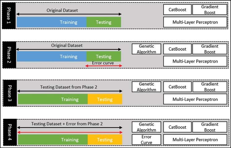
1894                                                                           CMC, 2021, vol.69, no.2

be successfully applied in many scientific research fields, especially those that manipulate large data
sets [1–3]. Many researchers have proposed using the residual compensation method to improve
the accuracy. Such as Su et al. [4] presented an improved collaborative research framework for
predicting solar power generation. An enhanced collection model is being proposed to improve
accurate predictions based on a new waste adaptation solution evolutionary optimization tech-
nique. They applied this solution to the solar projection using an asymmetric estimator. They
conducted extensive case studies on open data sets using multiple solar domains to demonstrate
Adaptive Residual Compensation integration technology’s benefits. In this article by Christian
et al. [5], the authors have proposed a new method of predicting thunderstorms using machine
learning model error as a feature. Their work’s basic idea is to use the two-dimensional optical
flow algorithm’s errors applied to meteorological satellite images as a function of machine learning
models. They interpret that an error in the speed of light is a sign of convection and can lead
to thunder and storms. They wrap using various manual steps to consider the proximity to
space. They practice various tree classification models and neural networks to predict lightning
over the next few hours based on these characteristics. They compared the effects of different
properties on the classification results to the predictive power of other models. Another work of
using machine learning model’s error is done by Zhang et al. [6]. The authors proposed a way
to train a single hidden layer feed-forward neural network using an extreme learning machine.
The proposed method presented found an effective solution to the regression problem due to the
limited modeling ability, the problem’s nonlinear nature, and the regression problem’s possible
nature. Extreme learning machine-based prediction error is unavoidable due to its limited modeling
capability. This article proposes new Extreme learning machines for regression problems, such
as the Extreme learning machine Remnant Compensation, which uses a Multilayered framework
that uses baselines to compensate for inputs and outputs other levels of correction. Post-Layer
Levels The proposed residual compensation-based-extreme learning machine may also be a general
framework for migration issues. However, they did not combine the proposed approach with deep
learning schemes.
     We have proposed a modified ensemble model to improve the forecast accuracy based on uti-
lizing the model’s error as a feature. This approach combines three models, namely CatBoost (CB),
Gradient Boost (GB), and Multilayer Perceptron (MLP). The ensembled CB-GB-MLP model’s
inner mechanism consists of generating a meta-data from Gradient Boosting and CatBoost models
to compute the final predictions using the Multilayer Perceptron network. A genetic algorithm
is used to obtain the optimal features to be used for the model. To prove the proposed model’s
effectiveness, we have used a four-phase technique using South Korea’s Jeju province’s actual
energy consumption data. Jeju Island is located on the southernmost side of the Korean peninsula.
The solar altitude remains high throughout the year, and in summer, it enters the zone of influence
of tropical air masses. It is situated in the Northwest Pacific Ocean, which is the Pacific Ocean’s
widest edge and is far from the Asian continent and is affected by the humid ocean [7]. The
foremost contributions of this article are to
    • combine three models of machine learning, namely Catboost, Gradient Boost, and Multi-
      layer Perceptron,
    • utilizing a genetic algorithm for the feature selection,
    • using error of model as a feature to improve the forecast accuracy.
   The remainder of the article is arranged as follows. Section 2 introduces preliminaries about
machine learning techniques used in this publication. Section 3 presents the four-stage proposed
methodology. Section 4 introduces the data collection, data analysis process, pre-processing, and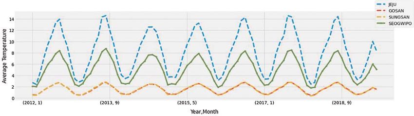
CMC, 2021, vol.69, no.2                                                                        1895

training. Section 5 presents the performance results of the proposed model evaluated using Jeju
energy consumption data. It also analyzes the results with the existing models. Lastly, we conclude
this article in the last conclusion section.

2 Preliminaries
      Artificial neural networks and machine learning provide better results than traditional sta-
tistical prediction models in various fields. Li [8] proposed a short-term forecasting model that
included extensive data mining and several continuous forecasting steps. To reduce the hassle with
noise in the short term, noise reduction methods are used based on analysis and reconstruction.
The phase reconstruction method is used to determine the dynamics of testing, training, and
neuron configuration of the artificial neural network (ANN). It also improves the ANN parameter
by applying a standard grasshopper optimization algorithm. The simulation results show that
the proposed model can predict the load in the short term using various measurement statistics.
However, other factors or parameters can be considered in the forecasting model to optimize the
short-term load prediction. The focus should be on developing data processing technology that
can manage short, erratic, and unstable data so users can manage the negative effects of noise.
We have proposed to ensemble three machine learning models followed by the genetic algorithm
optimization technique. This section introduces these three ML models according to their distin-
guished architecture and uses in literature, namely, Gradient Boosting model, CatBoost Model,
and Multilayer perceptron. Moreover, the Genetic algorithm and Ensemble model approaches are
also discussed.

2.1 Gradient Boosting Model
     Gradient Boosting model is a robust machine learning algorithm developed for various data
such as computer vision [9], chemical [10], and biological fields [11], and energy [12]. Tree-based
ensemble methods are gaining popularity in the field of prediction. In general, combining a
simple low return regression tree gives high accuracy of forecasting. Unlike other machine learning
techniques, Tree-based ensemble methods are considered black boxes. Tree-based grouping tech-
niques provide interpretable results, have little data processing, and handle many different types
of predictions. These features make tree-based grouping techniques an ideal choice for solving
travel time prediction problems. However, the application of the tree-based clustering algorithm in
traffic prediction is limited. In the article, Zhang et al. [13] use the Gradient Boosted Regression
Tree method to analyze and model highway driving time to improve prediction accuracy and
model interpretation. The gradient boosting method could strategically combine different trees
with improving prediction accuracy by correcting errors generated by the previous base model.
They discussed the impact of other parameters on model performance and variable input/output
correlations using travel time data provided by INRIX on both sections of the Maryland Highway.
They compared the proposed method with other hybrid models. The results show that gradient
boosting has better performance in predicting road transit times.
    In the study, Touzani et al. [14], a modeling method based on motor power consumption using
gradient boosting algorithm, is proposed. A recent testing program has been used in an extensive
data set of 410 commercial buildings to assess this method’s effectiveness. The model training
cycle evaluates the sample performance of different predictive methods. The results show that the
use of a gradient boosting compared to other machine learning models improves R-square and
root mean square error estimates by more than 80%.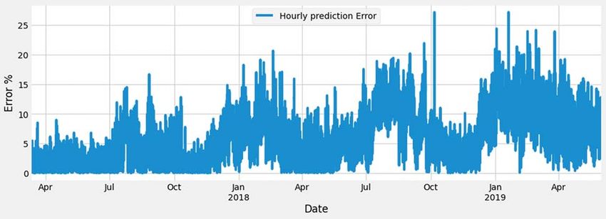
1896                                                                         CMC, 2021, vol.69, no.2

2.2 Catboost Model
     CatBoost is a gradient boosting algorithm-based open-source machine learning library. It
can successfully adjust the categorical features and use optimization instead of adjusting time
during training [15]. Another advantage of this algorithm is that it reduces the load and uses a
new system to calculate the leaves’ value in determining the shape of the tree [16]. It is mainly
used to solve logical problems and to solve functions efficiently. High-quality samples can be
obtained without parameter adjustment, and better results can be obtained by using a default
parameter, thereby reducing the conversion time. It also supports categorical parts without pre-
fixing non-numerical properties. In work by Diao et al. [17], catboost is used for short-term
weather forecasting using the datasets provided by Beijing Meteorological Administration. The
corresponding heat map, the removal of the recursive features, and the tree pattern are included
in selecting the features. Then they recommended the wavelet denoising of data and conducted
it before setting up a learning program. The test results show that compared to most in-depth
studies or machine learning methods, the catboost mode can shorten the connection time and
improve the system.

2.3 Multi-Layer Perceptron
    The multi-layer perceptron (MLP) consists of simple systems connected to neurons or nodes.
The nodes involved in the measurement and output signals result from the amount of material
available for that node, which is configured by the function or activation of a simple nonlinear
switch [18]. This is a feature of a straightforward nonlinear transition, allowing nonlinear embed-
ding functions in a multi-layer perceptron. The output is measured by connection weight and then
sent to the node in the next network layer as an input. The multi-layer perceptron is considered a
feed-forward neural network. In the study by Saha et al. [19], a multi-layer perceptron model was
used to predict the location of potential deforestation. Group-level success rates and levels are
compared to MLP. The described unit has been trained on 70% of deforestation; the remaining
30% have been used as test data. Distance to settlement, population growth, and distance to
roads were the most important factors. After assembling the MLP neural network calibration
with the hybrid classifier, the accuracy is increased. The described method can be used to predict
deforestation in other regions with similar climatic conditions.
    The MLP algorithm is trained to calculate and learn the weights, synapses, and neurons of
each layer [20]. MLP can be calculated using Eq. (1).
        n

yk = α       (ωi,k yi + ωk )                                                               (1)
         i=1

where the sigmoid function is α, ω is the weight, and k denotes the multi-layer perceptron model’s
output value, whereas yk is the output of the MLP. yi is given as the input for the first layer
to obtain the kth output. i indicates the number of the hidden layer from one to n. wi;k is the
connection between the ith hidden layer neuron and the kth output layer neuron.

2.4 Genetic Algorithm
    Genetic algorithm (GA) was inspired by Darwin’s theory of evolution, in which the survival
of organisms and more appropriate genes were simulated. GA is a population-based algorithm.
All solutions correspond to the chromosomes, and each parameter represents a gene [21]. GA
uses the (objective) fitness function to assess the fitness of everyone in the population. To improve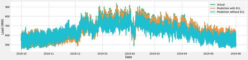
CMC, 2021, vol.69, no.2                                                                        1897

the poor solution, it is randomly selected using the optimal solution selection mechanism. The
GA algorithm starts with a random set. Populations can be generated from Gaussian random
distributions to increase diversity. Inspired by this simple natural selection idea, we use the
GA-algorithm roulette wheel to select them to create a new generation that matches the fitness
value assigned to an individual with probability. After choosing an individual with a limiting
factor, this is used to create a new generation. The last evolutionary factor in which one or more
genes are altered after making an eye solution. The mutation rate is set low because the high
GA mutation rate translates GA into a primitive random search term [22]. The mutation factor
maintains the diversity of the population by introducing different levels of randomness.

2.5 Ensemble Model
    Ensemble refers to the integration of prediction models to perform a single prediction.
Ensemble models can combine different weak predictive models to create more robust predictive
models [23–25]. The Blending Ensemble model uses not only the predicted value but also the origi-
nal feature. Fig. 1 shows the Graphical representation of the ensemble machine learning approach.
Where the dataset is training in different models, and their initial predictions are ensembled using
ensembler. In the article by Massaoudi et al. [26], the authors propose a framework by using Light
Gradient Boosting Machine (LGBM), eXtreme gradient Boosting machine (XGB), and Multilayer
Perceptron (MLP) for calculating effective short-term forecasts. The proposed method uses the
heap generalization method to identify potential changes in housing demand. The proposed
method is the combination of three models LGBM, XGB, and MLP. The Stacked XGB-LGBM-
MLP model’s inner mechanism consists of producing metadata from XGB and LGBM models to
compute the final predictions using the MLP network. The performance of the proposed XGB-
LGBM-MLP stack model is tested using two data sets from different sites. The proposed method
succeeded in reducing errors; however, the performance of the proposed method of stacking would
decrease up to 48 h slower.

         Figure 1: Graphical representation of the ensemble machine learning approach
1898                                                                         CMC, 2021, vol.69, no.2

     In the article by Park et al. [27], the author proposed a daily hybrid forecasting method based
on load feature decomposition. Short-term load forecasting can be implemented by adding public
pair forecasts composed of a combination of different intricate energy consumption patterns.
However, due to resource constraints for measurement and analysis, it may not be possible to
track all predicted sub-load usage patterns. The proposed method to prevent this feasibility focuses
on general characteristics, low load, and effective decomposition of typical pilot signals. Using the
proposed method, intricate energy consumption patterns can be grouped based on characteristic
contours, and the combined charges can be decomposed into sub-charges in the group. The
ensembled prediction model is applied to each sub load with the following characteristics to
predict the total charge by summarizing the expected cluster load. Hybrid prediction combines
CLD-based linear prediction with LSTM, which is superior to traditional methods of inaccurate
prediction. We use a hybrid method that combines conditional linear prediction of job type and
short-term, long-term memory regression to obtain a single prediction that decomposes feature
sub loads. Consider complex campus load data to evaluate the hybrid forecast of proposed
features during load decomposition. The evaluation found that the proposed plan outperformed
hybrid or similar historical-based forecasting methods. The sub-load can be measured in a limited
time period, but the decomposition technique can be applied to the extended training data through
virtual decomposition.

3 Proposed Methodology
    We have designed a four-phase strategy better to understand the impact of the error curve
learning technique. Fig. 2 shows the abstract of these four phases. In the first phase, we have
obtained the results by applying the CB-GB-MLP model. This approach combines three models,
namely CatBoost (CB), Gradient Boost (GB), and Multilayer Perceptron (MLP). The ensembled
CB-GB-MLP model’s inner mechanism consists of generating a meta-data from Gradient Boosting
and CatBoost models to compute the final predictions using the Multilayer Perceptron network.
In this phase, 70% of the original dataset is used for training purposes and 30% for testing. In the
second phase, we have utilized a GA-ensembled model with optimal features. The Input feature
for energy consumption forecasting consists of weather, time, and holidays.

                            Figure 2: Design of the four-phase strategy
CMC, 2021, vol.69, no.2                                                                        1899

     A genetic algorithm is used to obtain optimal features. The CB-GB-MLP model is then used
for the forecasting using the same data division scheme as used in phase 1. By applying the GA-
ensembled model, we obtained better performance results. By using Eq. (2), the error curve is
obtained at this stage. Where yt is the actual value of energy consumption and ŷt is the predicted
value.
         yt + ŷt
EC t =            × 100                                                                          (2)
            yt

    The third phase is for the comparison of the energy forecasting result with the proposed
ECL-based model. In this stage, we have used the testing dataset of phase 2 as the complete
dataset. Then we split this data into 70% and 30% for training and testing, respectively.
     The fourth stage is the final stage, where we have applied the genetic algorithm-based error
curve learning ensembled (GA-ECLE) model. For this phase, we have again used the testing
dataset of phase 2 as the complete dataset. Then we split this data again into 70% and 30%
for training and testing, respectively. However, this time we have used the error data obtained
at phase 2 as an input feature along with weather, time, and holiday features. By utilizing the
GA-ECLE model, we obtained comparatively good results. Fig. 3 explains the flow diagram of
the proposed GA-ECLE model. It starts with acquiring the input data from different sources,
then doing some feature engineering such as obtaining date features and then pre-processing it.
Preprocessing involves filling the missing values and converting the textual data into numeric data
for better training. The pre-processed data is then split into training and testing datasets. The
genetic algorithm is used to obtain optimal features; then, these optimal features are passed to
an ensembled model where test data is used to generate the error curve. The ensemble model is
trained again using the error curve and then obtaining the ensembled model’s optimal predictions.
y(t + 1) = f (y(t), . . . , y(t − m + 1) : F                                                     (3)

F = WF st , DF t , HF t , EF t                                                                   (4)

    Time series data is used to evaluate the performance of the proposed model. Eq. (3) is
used to estimate the predicted value of the next timestamp. The data we have used is hourly
based, so here t represents one Hour of time. y(t + 1) is the forecasted value at a given time,
y(t) represents the hourly load consumption at time t, and F represent the Features used to
estimate the future load value. As expressed in Eq. (4) there are four different classes of features
used. Where WFts , DFt , HFt , and EFt represents the weather, date, holiday, and error features,
respectively.
    There are four different weather stations in Jeju island named as Jeju-Si, Gosan, Sungsan,
and Seogwipo. Set of weather features from each weather station WFts , is represented in Eq. (5).
Meteorological features consist of Average temperature TAt , the temperature of dew point TDt ,
humidity HMt , wind speed W St , wind direction degree W Dt , atmospheric pressure on the ground
PAt discomfort index DIt , sensible temperature STt , and solar irradiation quantity SIt . Each
weather station is assigned a different weight factor according to its importance as described
in Eq. (6). Where the value of a is equal to 0:5, b and g is equal to 0:1 and d is 0:3.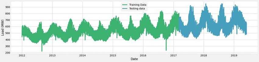
1900                                                                          CMC, 2021, vol.69, no.2

    j         g                       sp
WFt , β.WFt , γ .WFtss , and δWFt represent the set of weather features, according to the weather
stations of Jeju-Si, Gosan, Sungsan and Seogwipo respectively.
WF st = {TAt , TDt , HM t , WS t , WDt , PAt , DI t , ST t , SI t }                                (5)

                  j       g                 sp
WF st = α.WF t , β.WF t , γ .WF ss
                                t , δWF t                                                          (6)

                      Figure 3: Flow diagram of the proposed GA-ECLE framework

     Date features DFt can be extracted from the time-series data, which helps understand the
relation between the target value with respect to the time [28]. The set of date features as described
in Eq. (7) consist of Hour Ht, , month Mt, , year Yt, , Quarter Qt, and day of week DoWt, . Holidays
also greatly impact energy consumption; we have collected the holidays and make a set of holiday
features HFt as expressed in Eq. (8).
DF t = {H t, M t, Y t, Qt, DoW t, }                                                                (7)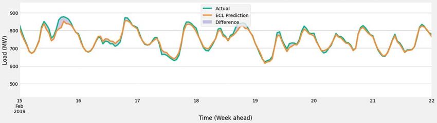
CMC, 2021, vol.69, no.2 1901
HF t = {HDt, SDC t, SDN t, } (8)
It contains holiday code HDt, , special day code SDCt, , special day name SDNt, . Holiday
code consists of holidays such as solar holiday, lunar holiday, election day, holidays interspersed
with workdays, alternative holidays, change in demand, and special days. Special days consist of
several holidays, including New Year’s Day, Korean army day, Korean New Year’s Day, Christmas,
workers’ day, children’s day, constitution day, and liberation day.
EF t = {EC t, AEC t, } (9)
yt + ŷt
AEC t = × 100 (10)
y t
We have proposed to use the error of model EFt as a feature. It contains two features
as explained in Eq. (9). ECt is calculated using Eq. (2) and absolute error curve AECt using
Eq. (10).
ff pv wp
Ltotal
t = Lt + Lbtm
t + Lt + Lt (11)
The target feature is the total hourly based load consumption Ltotal
t . Jeju island fulfills its
energy need from different sources. These sources include renewable and non-renewable energy
sources such as wind energy and solar energy. We have combined all the load consumption energy
ff
sources using Eq. (11). Where Lt shows the energy load using fossil fuel-based energy sources,
pv
Lbtm
t is for behind the meter sources. Lt represents load from photovoltaic sources and load
wp
consumption from wind energy sources are represented as Lt .
hybrid gb mlp
yt = C w . ycb
t + C w . yt + C w . yt (12)
M
C w = min (yt − ŷt ) , 0 ≤ Cw ≤ 1 (13)
t=1
The proposed hybrid model consists of three sub-models, Catboost, gradient boost, and multi-
hybrid
layer perceptron. The output of p roposed hybrid model yt is calculated using Eq. (12). Where
gb mlp
ycb
t ; yt ;
yt represents the output of Catboost, gradient boost and multi-layer perceptron models,
respectively. Cw represent the weight coefficientof each model and it is calculated using Eq. (13).
In this Eq. time t consist of M values, yt is the actual value and ŷt is the predicted output.
4 Forecasting Using GA-ECLE Model
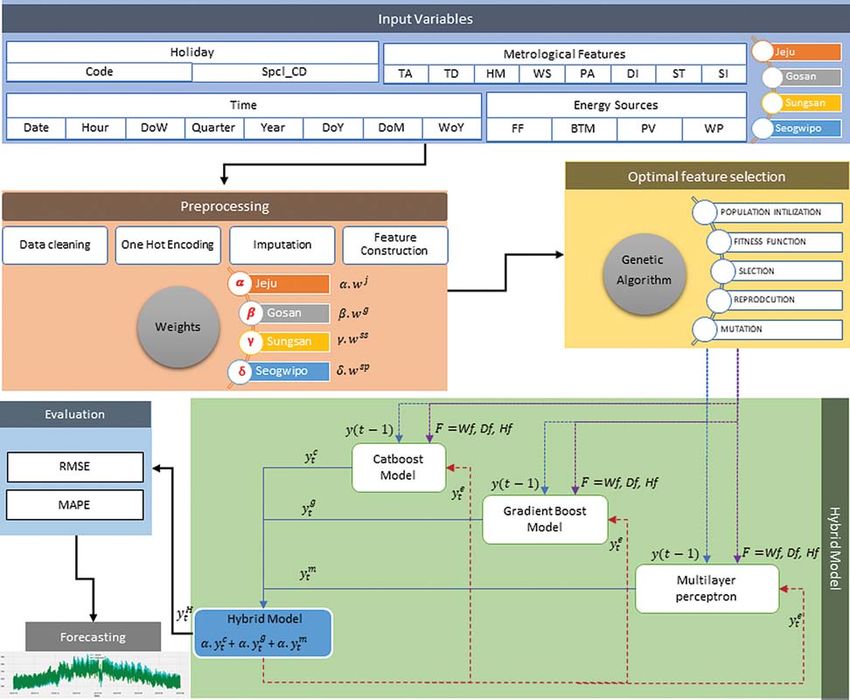
This section explains the complete data acquisition, data analysis, feature engineering, and
proposed model training. Fig. 4 shows the block diagram of the proposed forecasting framework
in the context of the Jeju island’s weather and energy consumption patterns. We have used the
actual energy consumption data of Jeju island South Korea. This island has four weather stations
named Jeju-si, gosan, sungsan, and seogwipo. Input variables for this model are of four different
types. First is the meteorological features from four different weather stations. The second is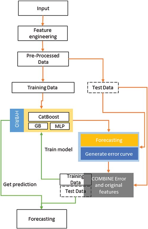
1902                                                                          CMC, 2021, vol.69, no.2

holidays, the third is time features, and the Fourth is energy sources, which comprise of fossil fuel-
based energy sources (FF), photovoltaic (PV), behind-the-meter (BTM), and wind power (WP)
energy sources.

                 Figure 4: Block diagram of the proposed forecasting framework

    Prepossessing this data involves different functions such as data cleaning, one-hot encoding,
imputation, and feature construction. We have also assigned different weights to the weather
features according to the impact of each weather station. This pre-processed data is used as input
for the genetic algorithm, which helps obtain optimal features according to their importance in
prediction. The initial number of features was 64, and it was reduced to 32 after applying the
genetic algorithm. We provided error and absolute error as features along with other holidays,
meteorological, and date features. These features served as input to the ECLE model. This enabled
model consists of three models, namely CatBoost (CB), Gradient Boost (GB), and Multilayer Per-
ceptron (MLP). The ensembled CB-GB-MLP model generates meta-data from Gradient Boosting
and CatBoost models and computes the final predictions using Multilayer Perceptron. We have
CMC, 2021, vol.69, no.2 1903
used different evaluation metrics such as root mean square error (RMSE) and mean absolute
percentage error (MAPE) to evaluate our proposed model.
The pseudo-code for the genetic algorithm-based error curve learning model is expressed
stepwise in Algorithm 1. It initializes with importing actual data files and libraries such as NumPy,
pandas, matplotlib. Then data is pre-processed using imputation, converting textual data into
numeric data using one-hot encoding and assigned weights α, β, γ , and δ to the meteorological
features according to the weather stations. A genetic algorithm is used to obtain optimal features.
The next step is to build and train an ensembled hybrid model modelhybrid . This model contains
CatBoostRegressor( ) and GradientBoostingRegressor( ) to obtain metadata and MLPRegressor( )
to compute the final predictions. The pre-processed data is divided into two parts one is for
training and the other for testing purposes. After training of this model, testing data is used
to generate an error curve. The error features are used to retrain the model and meteorological,
holiday, and date features. The final step is the evaluation and getting predictions using a trained
model.
Algorithm 1: Pseudo-code for Adaptive Error Curve Learning Ensemble Model
Step 1: Preliminaries
1: import libraries.
2: data = import CSV data file
3: Step 2: Preprocessing
4: Fill Null values
5: one hot encoding = encoding: fit (dff[“SDCt ])
j g sp
6: WF st = α.WF t , β.WF t , γ .WF ss t , δ.WF t
7: Apply genetic algorithm to get optimal features.
8: Step 3: Build and train model.
9: modelhybrid = BlendEnsemble( )
10: modelhybrid .addmeta (CatBoostRegressor( ))
11: modelhybrid .addmeta (GradientBoostingRegressor( ))
12: modelhybrid .add(MLPRegressor( ))
13: train = data.loc[data.index datesplit ].copy( )
15: modelhybrid .fit(trainX ; trainy )
16: Step 4: Get Error curve
y + ŷt
17: EC t = t × 100
yt
18: AEC t = |EC t |
19: Step 5: Retrain model using Error curve.
20: use error features and repeat Step 3.
21: Step 6: Evaluation and prediction
22: Evaluate the model using RMSE, MAE.
23: Prediction = modelhybrid .predict(testX )1904 CMC, 2021, vol.69, no.2
4.1 Exploratory Data Analysis
This section provides the exploratory data analysis to understand the patterns of data better.
The data provided by the Jeju energy corporation consist of different features. These features
include the energy consumption of different energy sources, weather information of four weather
stations, and holiday information. The total dataset consists of hourly-based energy consumption
from 2012 to mid of 2019. Fig. 5 shows the monthly energy consumption in the complete dataset.
Figure 5: Monthly average load consumption for each year
Each line shows a different year from 2012 to 2019. The X-axis represents the month, and
Y-axis represents the average energy consumption in MWs. Average energy consumption is low in
the month of November and high during August and January.
Fig. 6 shows the average weather temperate recorded at different Jeju island weather stations
after applying weight factors. Each line shows a different year weather station’s data. 2019. The
X-axis represents the time frame, and Y-axis represents the average temperature in Celsius.
Figure 6: Average temperature after applying weight for each weather station
Fig. 7 shows the energy consumption with respect to different seasons. Mean energy con-
sumption is highest during the winter season and lowest during the spring season.
Fig. 8 shows the mean energy consumption during each year. The gradual increase in
consumption can be observed from this chart.CMC, 2021, vol.69, no.2 1905
Figure 7: Season wise average load consumption
Figure 8: Year-wise average load consumption
Tab. 1 summarizes the variable used in the dataset. It contains the variable name, their
description, and measuring unit. Day of the week is represented from 0 to 6 starting from Sunday
as 0. This table shows the input data consist of Code of Day of the Week, Holiday Code, Special
Day Code, Special Day Name, Total Load, Temperature, Temperature of Due Point, Humidity,
Wind Speed, Wind Direction Degree, Atmospheric Pressure on the Ground, Discomfort Index,
Sensible Temperature, and Solar Irradiation Quantity. This data represents the problem adequately
because it contains various weather and day features that have a great impact on the energy
consumption.1906 CMC, 2021, vol.69, no.2
Table 1: Measuring units of features
Sr# Variable Name Unit
1 DFK_CD Code of Day of the Week sun(0) sat(6)
2 HOLDY_CD Holiday Code 0 = weekday, 1 = holiday
3 SPCL_CD Special Day Code –
4 SPCL_NM Special Day Name –
5 TOTAL_LOAD Total Load MW
6 TA Temperature â
7 TD Temperature of Due Point â
8 HM Humidity %
9 WS Wind Speed m/s
10 WD_DEG Wind Direction Degree deg
11 PA Atmospheric Pressure on the Ground hPa
12 DI Discomfort Index –
13 ST Sensible Temperature â
14 SI Solar Irradiation Quantity Mj/m2
Weekdays and holidays have assigned binary numbers, where weekday is represented as 0
and holiday as 1. Total load represents the hourly energy consumption in MW. Temperature, due
point temperature, and moderate temperature are measured in Celsius. Other features used are
humidity in percentage, wind speed in m/s, wind direction degree in deg, atmospheric pressure on
the ground in hpa, and solar irradiation quantity in Mj/m2 .
4.2 Training and Testing
The total dataset consists of hourly-based energy consumption from 2012 to 2019. It contains
64999 Rows. Tab. 2 summarizes the training and testing data for each phase.
Table 2: Training and testing data for each phase
Total Training Testing Training duration Testing duration
samples samples samples
Phase 1 64999 45476 19523 2012-01-01 to 2017-03-09 2017-03-10 to 2019-05-31
Phase 2 64999 45476 19523 2012-01-01 to 2017-03-09 2017-03-10 to 2019-05-31
Phase 3 19543 13680 5863 2017-03-10 to 2018-09-29 2018-09-30 to 2019-05-31
Phase 4 19543 13680 5863 2017-03-10 to 2018-09-29 2018-09-30 to 2019-05-31
Fig. 9 shows the graphical representation of testing and training data split for phase 1 and
phase 2. The green color is used to represent the training data, and the blue color shows the
testing phase data. For phase 1 and phase 2, we have used 62 months as training duration, which
contains 45476 rows. The last 26 months are used as testing data and to obtain the error curve,
which includes 19523 rows.CMC, 2021, vol.69, no.2 1907
Figure 9: Training and testing data for Phase 1 and Phase 2
The graphical representation of testing and training data split for phase 3 and phase 4 is
shown in Fig. 10. For phase 3 and phase 4, we have used 18 months 20 days of the training data,
consisting of 13680 rows from 10th of March 2017 to 29th of September 2018. We have used the
remaining last months as testing data, consisting of 5763 rows from the 30th of September 2018
to the 31st of May 2019.
Figure 10: Training and testing data for Phase 3 and Phase 4
5 Experimental Results and Evaluation
The accuracy of machine learning techniques must be verified before implementation in
the real-world scenario [29]. In this study, two methods are used to perform the accuracy and
reliability of assessment procedures. One is a graphic visualization, and the other is error metrics.
Error rating metrics used in the model evaluation method include mean absolute error (MAE),
mean absolute percentage error (MAPE), root mean square error (RMSE), and root mean squared
logarithmic error (RMSLE).
Fig. 11 shows the visual representation of Feature importance. The graph shows the order
of features with respect to their importance after applying the genetic algorithm. The X-axis
represents the feature importance score obtained using GA, and the Y-axis represents the feature’s
name. The data is collected on an hourly basis, so it can be observed that the hour feature is of
great importance in prediction, followed by the year feature. Then there are some weather features.
We have removed the features with less importance to improve the results. There were 64 features,
but after applying the genetic algorithm, the top 32 features are selected.
Fig. 12 shows the error curve obtained during phase 2. This error curve is used as an input
feature along with other weather and date features during phase 4. This graph shows the variation1908 CMC, 2021, vol.69, no.2
in error on an hourly basis. The X-axis shows the month, and Y-axis shows the percentage of
error.
1
MAE = (|ya − yp |) (14)
N
1
MSE = (ya − yp )2 (15)
N
1
RMSE = (ya − yp )2 (16)
N
1
RMSLE = (log(ya + 1) − log(yp + 1))2 (17)
N
Figure 11: Feature importance graph after applying genetic algorithm
The difference between prediction and actual values can be expressed as mean absolute error.
It can be calculated using Eq. (14). Where ya represents actual value and yp is the predicted value.
First, we calculate all absolute errors, add all up, and then divide by the total number of errors
expressed in the Eq. as N. The proposed model’s MAE is 3.05. Mean squared error is calculated
using Eq. (15). It represents the difference between the original value and the expected value [30].
First, we calculate all absolute errors, take the square of them, and then divide by the total
number of errors. The MSE of the proposed model is 115.09. RMSE is obtained by Eq. (16),CMC, 2021, vol.69, no.2 1909
It is calculated by the root of MSE. Where yp is the forecasted value obtained by the proposed
model, and ya is the actual load value. N represents the sample size in terms of numbers [31].
The RMSE of the proposed model is 5.05.
Figure 12: Error curve generated from phase 2
The root mean squared logarithmic error (RMSLE) is obtained by Eq. (17). The root mean
squared logarithmic error expressed the logarithmic relationship between the actual data value and
the model’s expected value. The RMSLE of the proposed model is 0.008.
Tab. 3 summarizes the error during all phases of experimental results. It covers the minimum,
maximum, and mean error of testing data according to each phase. From the table, it is evident
that there is a significant improvement in the results when we applied ECL. We have obtained
a maximum of 10.80% error, and the mean error recorded was 1.22%. We also performed a
comparison of the proposed GA-ECLE model with the state-of-the-art models including. Tab. 4
shows the comparison of different evaluation metrics.
Table 3: Comparison of error
Max % Min % Mean %
Phase 1 25.4532 0.00062 5.7576
Phase 2 (With GA) 23.8014 0.00027 4.9397
Phase 3 (Without ECL) 21.3264 0.00130 4.0231
Phase 4 (With ECL) 10.8014 0.00027 1.2297
Table 4: Model accuracy evaluation metrics
Sr Name MAE MSE RMSE RMSLE
1 GradientBoost 7.86 295.95 13.004 0.22
2 CatBoost 13.75 517.92 22.75 0.038
3 Multilayer Perceptron 40.50 1525.27 67.02 0.115
4 LSTM 37.33 1405 63.59 0.108
5 Xgboost 19.94 750.98 32.99 0.056
6 Support Vector Regressor 30.88 1162.73 51.09 0.086
7 Proposed 3.05 115.09 5.05 0.0081910 CMC, 2021, vol.69, no.2
The prediction result of testing data is also illustrated using graphs. In Phase 4, data from
the 30th of September 2018 to the 31st of May 2019 is used as testing data. Fig. 13 represents
the graphical comparison between the results of applying ECL.
Figure 13: Comparison of Actual test data and prediction with and without ECL
Green lines show the actual load values, orange lines show the prediction result after applying
ECL, and cyan color lines represent the prediction using the same model but without ECL.
To better visualize the results, we have selected two different time frames. One is 48 h, and
the other is one week or 168 h. Fig. 14 shows the results between 48 h, which comprised from
the 20th of May 2019 to the 22nd of May 2019. Fig. 15 shows the graphical representation of
actual predictions and their difference for one week. The week we selected starts on the 15th of
February 2019 and ends on the 21st of February 2019. In both figures, the green line shows the
actual load consumption, and the orange line represents the prediction with ECL. Whereas the
difference in prediction and actual consumption is illustrated using purple color.
Figure 14: Comparison of 48 h ahead prediction with and without ECL
Figure 15: Comparison of the week ahead prediction with and without ECLCMC, 2021, vol.69, no.2 1911
6 Conclusions
This research presents a novel genetic algorithm-based adaptive error curve learning ensemble
model. The proposed technique sorts random variants to improve energy consumption predictions
according to a machine learning-based ensembled approach. The modified ensemble model use
error as a function to improve prediction accuracy. This approach combines three models: Cat-
Boost, Gradient Boost, and Multilayer Perceptron. A genetic algorithm is used to obtain the best
properties available in the model. To prove the proposed model’s effectiveness, we used a four-step
technique that utilized Jeju Island’s actual energy consumption data. In the first step, the CB-GB-
MLP model was applied, and the results were obtained. In the second phase, we used a large,
full-featured GA model. The third step is to compare the energy prediction results with the pro-
posed ECL model. The fourth step is the final step of applying the GA-ECLE model. Extensive
experimental results have been presented to show that the proposed GA-ECLE model is superior
to the existing machine learning models such as GradientBoost, CatBoost, Multilayer Perceptron,
LSTM, Xgboost, and Support Vector Regressor. The results of our approach seem very promising.
We obtained a mean error of 1.22%, which was 5.75%, without using the proposed approach. We
have presented the results in a graphical way along with the statistical comparison. The empirical
results seem mostly favorable for the applicability of the proposed model in the industry. In the
future, other features can be added, such as the impact of the population using electricity and
the number of electric vehicles.
Funding Statement: This research was financially supported by the Ministry of Small and Medium-
sized Enterprises (SMEs) and Startups (MSS), Korea, under the “Regional Specialized Industry
Development Program (R&D, S2855401)” supervised by the Korea Institute for Advancement of
Technology (KIAT).
Conflicts of Interest: The authors declare that they have no conflicts of interest to report regarding
the present study.
References
[1] G. Alova, P. A. Trotter and A. Money, “A machine-learning approach to predicting Africa’s electricity
mix based on planned power plants and their chances of success,” Nature Energy, vol. 6, no. 2, pp.
158–166, 2021.
[2] X. Shao, C. S. Kimand and D. G. Kim, “Accurate multi-scale feature fusion cnn for time series
classification in smart factory,” Computers, Materials & Continua, vol. 65, no. 1, pp. 543–561, 2020.
[3] D. Zhou, S. Ma, J. Hao, D. Han, D. Huang et al., “An electricity load forecasting model for integrated
energy system based on bigan and transfer learning,” Energy Reports, vol. 6, pp. 3446–3461, 2020.
[4] H.-Y. Su, T.-Y. Liu and H.-H. Hong, “Adaptive residual compensation ensemble models for improving
solar energy generation forecasting,” IEEE Transactions on Sustainable Energy, vol. 11, no. 2, pp. 1103–
1105, 2019.
[5] C. Schön, J. Dittrich and R. Müller, “The error is the feature: How to forecast lightning using a model
prediction error,” in Proc. of the 25th ACM SIGKDD Int. Conf. on Knowledge Discovery & Data Mining,
2019.
[6] J. Zhang, W. Xiao, Y. Li and S. Zhang, “Residual compensation extreme learning machine for
regression,” Neurocomputing, vol. 311, pp. 126–136, 2018.
[7] J.-H. Won, Lee, J.-W. Kim and G.-W. Koh, “Groundwater occurrence on Jeju island, Korea,” Hydro-
geology Journal, vol. 14, no. 4, pp. 532–547, 2006.
[8] C. Li, “Designing a short-term load forecasting model in the urban smart grid system,” Applied Energy,
vol. 266, pp. 114850, 2020.1912 CMC, 2021, vol.69, no.2
[9] F. Zhang, B. Du and L. Zhang, “Scene classification via a gradient boosting random convolutional
network framework,” IEEE Transactions on Geoscience and Remote Sensing, vol. 54, no. 3, pp. 1793–1802,
2015.
[10] J. Lu, D. Lu, X. Zhang, Y. Bi, K. Cheng et al., “Estimation of elimination half-lives of organic
chemicals in humans using gradient boosting machine,” Biochimica et Biophysica Acta (BBA)-General
Subjects, vol. 1860, no. 11, pp. 2664–2671, 2016.
[11] X. Lei and Z. Fang, “Gbdtcda: Predicting circrna-disease associations based on gradient boosting
decision tree with multiple biological data fusion,” International Journal of Biological Sciences, vol. 15,
no. 13, pp. 2911, 2019.
[12] H. Lu, F. Cheng, X. Ma and G. Hu, “Short-term prediction of building energy consumption employing
an improved extreme gradient boosting model: A case study of an intake tower,” Energy, vol. 203,
pp. 117756, 2020.
[13] Y. Zhang and A. Haghani, “A gradient boosting method to improve travel time prediction,” Trans-
portation Research Part C: Emerging Technologies, vol. 58, pp. 308–324, 2015.
[14] S. Touzani, J. Granderson and S. Fernandes, “Gradient boosting machine for modeling the energy
consumption of commercial buildings,” Energy and Buildings, vol. 158, pp. 1533–1543, 2018.
[15] P. W. Khan, Y.-C. Byun, S.-J. Lee, D.-H. Kang, J.-Y. Kang et al., “Machine learning-based approach to
predict energy consumption of renewable and non-renewable power sources,” Energies, vol. 13, no. 18,
pp. 4870, 2020.
[16] A. V. Dorogush, V. Ershov and A. Gulin, “Catboost: Gradient boosting with categorical features
support,” arXiv preprint arXiv: 1810.11363, 2018.
[17] L. Diao, D. Niu, Z. Zang and C. Chen, “Short-term weather forecast based on wavelet denoising and
catboost,” in Chinese Control Conf., Guangzhou, China, IEEE, 2019.
[18] P. Wang, B. A. Hafshejani and D. Wang, “An improved multi-layer perceptron approach for de-tecting
sugarcane yield production in iot based smart agriculture,” Microprocessors and Microsystems, vol. 82,
pp. 103822, 2021.
[19] S. Saha, G. C. Paul, B. Pradhan, K. N. Abdul Maulud, A. M. Alamri et al., “Integrating multi-
layer perceptron neural nets with hybrid ensemble classifiers for deforestation probability assessment in
eastern India,” Geomatics Natural Hazards and Risk, vol. 12, no. 1, pp. 29–62, 2021.
[20] A. A. Tamouridou, T. K. Alexandridis, X. E. Pantazi, A. L. Lagopodi, J. Kashefi et al., “Applica-
tion of multi-layer perceptron with automatic relevance determination on weed mapping using UAV
multispectral imagery,” Sensors, vol. 17, no. 10, pp. 2307, 2017.
[21] P. W. Khan and Y.-C. Byun, “Genetic algorithm based optimized feature engineering and hybrid
machine learning for effective energy consumption prediction,” IEEE Access, vol. 8, pp. 196274–196286,
2020.
[22] M. K. Amjad, S. I. Butt, R. Kousar, R. Ahmad, M. H. Agha et al., “Recent research trends in genetic
algorithm based flexible job shop scheduling problems,” Mathematical Problems in Engineering, vol.
2018, 2018.
[23] X. Wu, Y. Wang, Y. Bai, Z. Zhu, A. Xia et al., “Online short-term load forecasting methods using
hybrids of single multiplicative neuron model, particle swarm optimization variants and nonlinear
filters,” Energy Reports, vol. 7, pp. 683–692, 2021.
[24] S. Goda, N. Agata and Y. Matsumura, “A stacking ensemble model for prediction of multi-type tweet
engagements,” in Proc. of the Recommender Systems Challenge 2020, Brazil, pp. 6–10, 2020.
[25] N. Somu, G. R. MR and K. Ramamritham, “A hybrid model for building energy consumption
forecasting using long short term memory networks,” Applied Energy, vol. 261, pp. 114131, 2020.
[26] M. Massaoudi, S. S. Refaat, I. Chihi, M. Trabelsi, F. S. Oueslati et al., “A novel stacked generaliza-
tion ensemble-based hybrid lgbm-xgb-mlp model for short-term load forecasting,” Energy, vol. 214,
pp. 118874, 2020.
[27] K. Park, S. Yoon and E. Hwang, “Hybrid load forecasting for mixed-use complex based on the
characteristic load decomposition by pilot signals,” IEEE Access, vol. 7, pp. 12297–12306, 2019.CMC, 2021, vol.69, no.2 1913
[28] P. W. Khan, Y.-C. Byun, S.-J. Lee and N. Park, “Machine learning based hybrid system for imputation
and efficient energy demand forecasting,” Energies, vol. 13, no. 11, pp. 2681, 2020.
[29] G. A. Tahir and C. K. Loo, “An open-ended continual learning for food recognition using class
incremental extreme learning machines,” IEEE Access, vol. 8, pp. 82328–82346, 2020.
[30] Z. Wang, T. Zhang, Y. Shao and B. Ding, “LSTM-Convolutional-BLSTM encoder-decoder network for
minimum mean-square error approach to speech enhancement,” Applied Acoustics, vol. 172, pp. 107647,
2021.
[31] R. Ünlü and E. Namlı, “Machine learning and classical forecasting methods-based decision support
systems for covid-19,” Computers, Materials & Continua, vol. 64, no. 3, pp. 1383–1399, 2020.You can also read