Agricultural and Forest Meteorology - Research UNE
←
→
Page content transcription
If your browser does not render page correctly, please read the page content below
Agricultural and Forest Meteorology 303 (2021) 108369
Contents lists available at ScienceDirect
Agricultural and Forest Meteorology
journal homepage: www.elsevier.com/locate/agrformet
Block-level macadamia yield forecasting using spatio-temporal datasets
James Brinkhoff *, Andrew J. Robson
Applied Agricultural Remote Sensing Centre, University of New England, Armidale 2350 NSW Australia
A R T I C L E I N F O A B S T R A C T
Keywords: Early crop yield forecasts provide valuable information for growers and industry to base decisions on. This work
Macadamia considers early forecasting of macadamia nut yield at the individual orchard block level with input variables
Remote sensing derived from spatio-temporal datasets including remote sensing, weather and elevation. Yield data from
Yield forecasting
2012–2019, for 101 blocks belonging to 10 orchards, was obtained. We forecast yield on each test year from
Climate
Statistical models
2014–2019 using models trained on data from years prior to the test year. Forecasts are generated in January, for
Machine learning the coming harvest in March–September. A linear model using ridge regularized regression produced consistently
good predictions compared with other machine learning algorithms including lasso, support vector regression
and random forest. Adding meteorological variables offered little improvement over using only remote sensing
variables. The 2019 forecast root mean square error at the block level was 0.8 t/ha, and mean absolute per
centage error was 20.9%. When block level predictions were aggregated across the multiple orchards per region,
production prediction errors were between 0–15% from 2016–2019. The ridge regression model can be easily
implemented in GIS platforms to deliver block-level yield forecast maps to end users.
local variation in tree health, soil, landscape and micro-climate (Fel
derhof and Gillieson, 2011; Johansen et al., 2020).
Macadamias are a high value tree nut crop, native to Australia. They Analytic yield prediction methods can be grouped into process-based
are now grown in many countries and the industry is experiencing rapid and statistical models (Lobell and Burke, 2010b). Process-based
expansion as demand rises (Stephenson, 2005). In 2016, the major methods model factors such as light interception, photosynthesis,
producers were Australia (25% of global production with 46,000 tonnes respiration, carbon assimilation and how this carbon is partitioned into
of nut-in-shell at 10% moisture), South Africa (23%), Kenya (15%) and non-harvested and harvested components of a crop (Marcelis et al.,
Hawaii (9%) (Topp et al., 2019). China’s production is rapidly 1998). These offer deep insight into the biological and environmental
increasing. The area of production in Australia in 2017 was estimated to factors driving yield variability. They can therefore be used to predict
be 23,000 hectares (Brinkhoff and Robson, 2020). the impact of factors such as climate change on crop production, and to
In Australia, most macadamias are harvested between March and make predictions in new regions. However, due to the complexity and
September, depending on region and maturity. The mature nuts fall interaction of biological processes, and the possibility of unforeseen
from the trees, and are gathered at regular intervals during the harvest factors impacting these processes in new regions, they are difficult to
period by finger-wheel harvesters (O’Hare et al., 2004). There is great parameterize and to obtain sufficiently accurate predictions for industry
interest in the industry to have early (January) and accurate forecasts of use. Some works use remote sensing data to improve the parameteri
yield (Mayer et al., 2019). This allows the industry to forecast total crop, zation of physiological models (Maselli et al., 2012), however no
and therefore adjust their marketing strategies and logistics planning. comprehensive process-based model of macadamia trees is currently
Growers are interested in yield predictions as they will aid finance, in available, which necessitates using another approach.
surance and logistic decisions. Yield prediction models may also provide On the other hand, statistical models describe yield as a function of
information on the drivers of yield variability, and thus offer potential combinations of input variables. Such models are parameterized based
for optimizing yield if variables that can be managed are identified. on historical observations (Zhang et al., 2019). Inputs to such a model
Spatial yield analysis facilitates precision agriculture applications by may include meteorological variables, remote sensing, soil characteris
adjusting management spatially to achieve optimal yields, considering tics, elevation, gradient as well as variables derived from crop factors
* Corresponding author.
E-mail address: james.brinkhoff@une.edu.au (J. Brinkhoff).
https://doi.org/10.1016/j.agrformet.2021.108369
Received 4 September 2020; Received in revised form 17 December 2020; Accepted 8 February 2021
Available online 24 February 2021
0168-1923/© 2021 The Authors. Published by Elsevier B.V. This is an open access article under the CC BY-NC-ND license
(http://creativecommons.org/licenses/by-nc-nd/4.0/).
J. Brinkhoff and A.J. Robson Agricultural and Forest Meteorology 303 (2021) 108369
such as variety, layout and management practices (fertilizer and water to produce a yield forecast model, rather they analyzed spatial vari
application, pruning, pollination). The detail of the physical processes ability using high-resolution imagery.
leading to yield outcomes are not described by statistical models, Macadamia yields are highly variable from year-to-year (McFadyen
however they may provide some insight into the input factors driving et al., 2004), with suggested causes being climatic variation (Mayer
yield variation (Jin et al., 2020). They are typically based on linear et al., 2019) and carbohydrate cycling (Huett, 2004). However, the
methods (for example, ordinary least squares) or machine-learning ap precise causes and methods of predicting and reducing this variation are
proaches (for example tree-based models such as random forests (RF), still unknown, which necessitates accumulation of high quality yield
support vector regression (SVR) or artificial neural networks (ANN)) data from many years and the use of controlled experiments to establish
(Zhang et al., 2019). One limitation is that they may fail to predict yield causal links between yield and management or environmental factors
when the input factors, such as weather, fall outside of the range of (Huett, 2004).
conditions encountered in the historical data the model was trained on In this study, we aim to produce a macadamia yield forecast model at
(Deines et al., 2020; Marcelis et al., 1998). the orchard block level. The forecasts are produced in a timeframe useful
Much research has focused on forecasting yield of annual crops, such for growers, at least two months before harvest begins. The predictor
as maize (Kang et al., 2020), cotton (Filippi et al., 2020) and rice variables come from publicly available spatio-temporal datasets, so that
(Setiyono et al., 2019). Predictor variables for such models typically predictions can be generalized to new orchards and areas. First, we
make use of in-season data. The yield of fruit and nut tree crops how investigated the importance of the possible yield predictor variables
ever, often have dependence on multiple years of factors such as weather from remote sensing, meteorological and spatial datasets. Then, forecast
due to their ability to store resources such as carbohydrates (Stephenson models of a range of complexities were trained using historical block
et al., 1989), and exhibit complex behavior such as biennial bearing level data and machine learning approaches. Forecasts were assessed,
(Huett, 2004). There are relatively few studies reporting tree crop yield before selecting and implementing a final model.
forecasting compared with those focussing on annual crops (van Klom
penburg et al., 2020). 1. Study area
The impact of particular climatic and management factors on mac
adamia yield have been the subject of some studies. For example Tro The study included 8 years of yield data (2012–2019) from 101 or
choulias and Lahav (1983) found optimum growth between 20 and 25 chard blocks belonging to 10 orchards across 3 significant Australian
∘
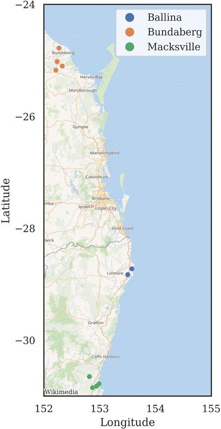
C. Smit et al. (2020) showed that CO2 assimilation was maximum with macadamia growing regions. The locations are shown in Fig. 1 and
leaf-to-air vapour pressure deficits between 1–2.5 kPa. McFadyen et al. encompass a range of climate conditions and orchard management
(2004) found macadamia yield increases with tree volume up to 43,500 strategies. We define a block as an area in an orchard that has had yield
m3 /ha (corresponding to light interception of 94%) and decreases with data recorded, typically with uniform management and plant year.
tree crowding above this value, though no decline in quality with The growers supplied maps of their blocks, which were digitized.
crowding was observed. Stephenson et al. (2000) found optimum yields They also provided production data, with values reported as kilograms
and quality are obtained at lower nitrogen rates, recommending 355 g (kg) of nut-in-shell (NIS) at 10% moisture (O’Hare et al., 2004), per
nitrogen application in late autumn to early winter and that rainfall block and per year. A summary of data from each region is shown in
during harvest negatively impacted quality. Stephenson et al. (1986a) Table 1. The range of planting dates spans 25 years for the Ballina
found that weather is not as important in describing yield variation as blocks, 4 years for the Bundaberg blocks and 19 years for the Macksville
leaf nutrients and flushing characteristics and soil zinc levels. A model of blocks. In the Macksville region, trees were older on average, and yields
8 parameters (not including weather) was able to account for 58.2% of
the observed yield variation, while a model with weather variables
described 40.3% of the yield variation.
Currently, yield forecasts for Australian macadamia farms are pro
vided by experienced agronomists and growers using information
including weather, flower and nut counts. However, this method is
subjective, and is limited in the amount of temporal and spatial
(considering only selected trees within an orchard) information it can
utilise.
At a larger scale, work on predicting yield over large regions of the
macadamia industry in Australia using statistical models is ongoing
(Mayer et al., 2019). These models take data on total production per
region per year, and fit models using input variables including weather,
market price, tree age and total area. Recent work has used satellite data
to improve accuracies of the estimates of total planted area and tree age
per region (Brinkhoff and Robson, 2020) to aid regional yield
predictions.
The potential of using high-resolution remote sensing imagery to
predict macadamia yield variability has been examined by Robson et al.
2017. Models were calibrated using total nut weight measured from
trees selected from three vigour zones within each study block. While a
positive relationship between tree vigour and yield was identified across
a number of locations and seasons, the remotely sensed vegetation index
that best predicted yield varied between orchard blocks. For each site
and season, the optimal vegetation indices were able to describe be
tween 69 and 86% of the spatial variation of yield. Similarly, Johansen
et al. (2020) assessed macadamia tree condition using high-resolution
imagery and showed that it is difficult to generalise a model devel
oped from one location or variety to another. These studies did not aim
Fig. 1. Location of study orchards from each of the growing regions.
2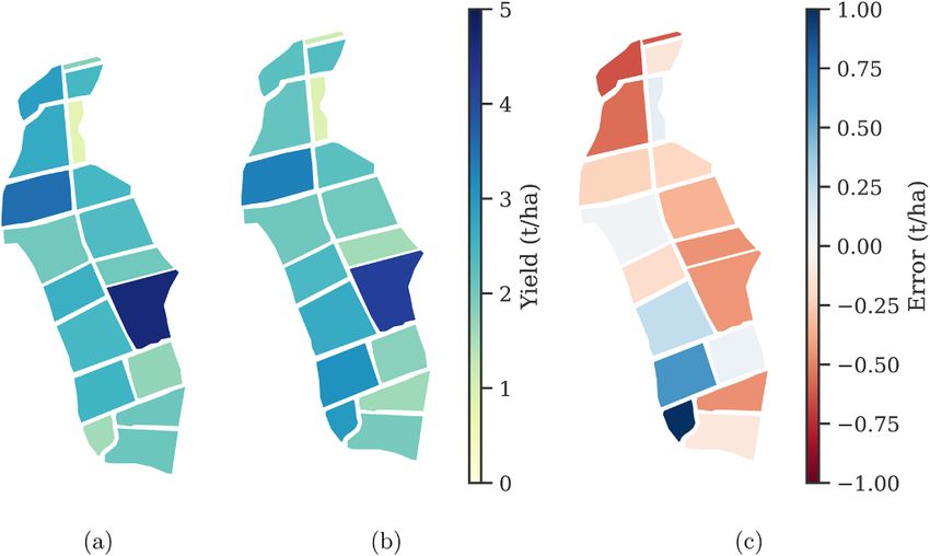
J. Brinkhoff and A.J. Robson Agricultural and Forest Meteorology 303 (2021) 108369
Table 1 2. Methods
Number of blocks in each region, data points (sum of blocks by years of recorded
yield data), and the average block areas, planting years and yields. 2.1. Spatio-temporal data
Region Blocks Datapoints Mean area Rangeplant Mean yield
(ha) years (t/ha) Spatio-temporal datasets were accessed and processed in Google
Ballina 39 125 4.2 1989–2014 2.9 Earth Engine (GEE) (Gorelick et al., 2017). Spatial data aggregated per
Bundaberg 31 203 9.1 2004–2008 3.3 block included:
Macksville 31 147 7.0 1991–2010 2.1
All 101 475 7.1 2003 (mean) 2.8
• Smoothed elevation model (from Geoscience Australia, derived from
LiDAR 5m grid, as available in GEE), from which the slope, north-
lower compared with the northern Bundaberg region. Most Bundaberg facing slope and east-facing slope were calculated. The elevation
orchards are irrigated, whereas Ballina and Macksville orchards mainly difference between orchards was not significant, they were all close
rely on rainfall. to sea-level.
The number of block yield data points per region and year is shown • Tree planting year model. This was generated from Landsat data
in Fig. 2b. There was no data recorded for Ballina before 2014, and no using the methods in (Brinkhoff, Robson, 2020), from which the
data for Macksville in 2014. One of the Ballina orchards suffered a median tree age per block per year was calculated. We used this
hailstorm which affected 2018 yields, so that data was omitted. We have model instead of grower-supplied tree ages so the yield forecast
also omitted Ballina data from 2017, because of the severe rainstorms model could be applied to orchards for which we don’t have access to
during harvest that washed much of the fallen nut away. Future work grower-supplied tree age data.
could include rolling updates to forecasts to capture adverse affects such
as this during the long harvest period, however the current models are Two spatio-temporal datasets were used, also available in GEE:
aimed at providing estimates of potential yield in January, before har
vest starts. The minimum number of annual data points was 37 in 2012, • Landsat 5, 7 and 8 tier 1 scenes, from 1988–2019 at 30 meter reso
and a maximum of 93 in 2019. lution. The scenes are available as surface reflectance in GEE
The wide spatio-temporal variation in yields between years, regions (atmospherically corrected using the respective USGS procedures).
and blocks is shown in Fig. 2a. Block yields range from close to 0 t/ha to The images in GEE also contain a cloud mask produced using USGS
almost 7 t/ha. Some of the yield variability may be explained by tree age CFMASK, which was applied to all images. We investigated harmo
and climatic differences. Four key meteorological variables for each nizing the reflectances measured by the TM, ETM+ and OLI sensors
region are shown in Fig. 3. There is significant variation in rainfall from using the equations proposed by Roy et al., 2016, however these did
year-to-year across all regions. 2019 was in the midst of a severe drought not result in improved model predictions, so we omitted this step. All
with low rainfall and high temperatures and evapotranspiration. In normalized difference spectral indices (NDSIs) were calculated from
general, Bundaberg experiences lower rainfall and higher evapotrans combinations of input bands (blue=b, green=g, red=r, near
piration than other regions, which necessitates irrigation. There are infra-red=nir, shortwave infra-red 1=swir1 and shortwave infra-red
significant differences in maximum and minimum temperatures be 2=swir2). This yields 15 linearly-independent NDSIs. For example,
tween regions. Thus, Fig. 3 shows that our dataset encompasses a wide ND(NIR,R)=(NIR-R)/(NIR+R) corresponds to NDVI.
range of climatic conditions, due to both season and region. • SILO (Jeffrey et al., 2001), a 5 km resolution daily meteorological
Fig. 3e shows the green normalized difference vegetation index dataset, interpolated from weather station observations. Variables
(GNDVI, Gitelson et al. 1996), computed from the remote sensing data. include minimum and maximum temperatures (Tmin and Tmax),
This shows the variability of tree reflectance from year-to-year, which solar radiation (SolarRad), vapour pressure deficit (VPD), reference
may be caused by a combination of factors such as climate, manage evapotranspiration (ETo) and rainfall (Rain). The SILO dataset is
ment, tree age and canopy cover. updated regularly in GEE, and so can be used to produce yield
forecasts in the required timeframe.
Landsat satellite data was selected because of its relatively high
resolution compared with other data that covers a similar historical
timeframe. SILO is used because of its ability to capture spatial variation
Fig. 2. (a) Distribution of all block yields per year and region. (b) The number of block yield data points per year and region.
3
J. Brinkhoff and A.J. Robson Agricultural and Forest Meteorology 303 (2021) 108369
Fig. 3. Annual aggregate meteorological and remote sensing variables for each region. (a) Average maximum temperature. (b) Total rainfall. (c) Average minimum
temperature. (d) Total reference evapotranspiration. (e) Average GNDVI.
at a reasonable scale and its availability within GEE, which facilitates its (annual and quarterly) using the mean operation. The Landsat variables
use in generation of annual yield prediction maps. were aggregated using the median operation, as this avoided the pos
Considering the different temporal frequency of the Landsat and sibility of outlying pixels in the time-series stack (such as from
SILO data, and the fact that cloud sometimes caused monthly Landsat unmasked clouds and shadows) skewing the aggregated values.
mosaics to be totally masked over a number of blocks, we aggregated The squared values for all these spatio-temporal variables were
each of the spatio-temporal datasets at two temporal scales. Firstly, per calculated and added to the set of predictor variables, as shown in Fig. 4.
year and secondly per quarter. Quarters were defined as s1=January- Including these nonlinear terms improved the yield forecasts.
March, s2=April-June, s3=July-September and s4=October-December. The spatial mean per block and per year of each of the variables was
Macadamia phenology varies with climate (Stephenson et al., 1986b), computed. The resulting table was then widened, so that each row
but s1 approximately encapsulates summer leaf flush, s2 flower initia included the aggregated spatio-temporal values for the two years pre
tion, s3 spring flush and peak flowering and s4 nut growth and begin vious to the yield prediction year (y1 and y2). This was merged with the
ning of oil accumulation (Schaffer and Andersen, 2018). Other temporal tables of the recorded yields for the current yield year (y0) and block
aggregations were also assessed before settling on quarterly aggrega areas. The resulting table was used in the training and testing of the yield
tion. For example, using only three four-month periods produced less prediction models.
accurate forecasts. Using five two-month periods had the disadvantage Importantly, the models are true forecast models in that yield in the
that many blocks had no valid image data for some periods due to cloud. current year is forecast without using any data from the current year. It
The SILO variables were aggregated at the two temporal scales is based only on variables aggregated from two previous years (y1 and
4J. Brinkhoff and A.J. Robson Agricultural and Forest Meteorology 303 (2021) 108369
2ŝ
LCCC = YY
( )2 (4)
2 2
s + sY + Y ̂− Y
̂Y
where ŝ is the covariance between predicted and measured yields, s2
YY ̂
Y
and s2Y are the variances of the predicted and measured yields respec
tively, and Y
̂ and Y are the means of the predicted and measured yields.
The mean absolute percentage error gives an easily interpretable
assessment of average prediction accuracy relative to average yields
(note, we use the weighted definition of MAPE throughout):
N ⃒ ⃒
1 ∑ ⃒ ̂ n ⃒⃒ × 100
MAPE = ⃒Yn − Y (5)
NY n=1
The root-mean squared error penalizes larger errors more than mean
Fig. 4. Model variables created from spatial and spatio-temporal datasets. absolute error, and is therefore used to select between models and as the
Abbreviations are defined in Section 2.1. scoring metric for optimizing model tuning parameters:
√̅̅̅̅̅̅̅̅̅̅̅̅̅̅̅̅̅̅̅̅̅̅̅̅̅̅̅̅̅̅̅̅̅̅̅̅̅̅̅̅
1 ∑N ( )2
y2). Data from the two previous years was used as macadamia yield RMSE = Yn − Y ̂n (6)
depends on previous management and climatic conditions. For example, N n=1
topping (pruning the tops of trees) reduces yield and can take several
2.2.2. Cross validation and model testing
years to recover from, and carbohydrate storage from previous years can
The model selection, training and testing procedure is illustrated in
affect current yield (Huett (2004)).
Fig. 5. Grid-search cross-validation (CV) in the SciKit-Learn Python
Fig. 4 shows the input variables and the temporal aggregations. The
package (Pedregosa et al., 2011) was used to select model tuning pa
result was 424 variables in total, consisting of 4 spatial variables, 300
rameters, such as α of lasso and ridge regression, or the number of trees
variables derived from Landsat observations and 120 from the SILO
for random forest. We note that the number of predictor variables (424)
data.
is similar to the total number of samples available for training models (<
475, Table 1), making proper cross validation procedures coupled with
machine learning algorithms that are able to deal with this p ≈ n sce
2.2. Modeling methods
nario crucial to avoid over-fitting to training data.
Cross validation was performed using the leave-one-group-out
2.2.1. Model evaluation and optimization metrics
method of SciKit-Learn, with the groups split by year, which we call
The actual macadamia production (P) in tonnes (t) for a given area is
leave-one-year-out (LOYO). This LOYO CV method produces a model
defined as:
that generalizes to an unseen year better than randomly splitting data
∑
N into training and validation sets. The latter method often results in an
P= An Yn (1) overfit model, because the model tuning parameters are optimized for
predictions for the unrealistic case of data from the test year being
n=1
where An is the area of individual units, such as pixels, blocks, farms or available for training (Brinkhoff et al., 2019). For each test year, only
regions, measured in hectares (ha). Yn is the yield in tonnes/ha for each data from years prior to the test year were used to train the models. So
of those units. The goal is to find a predictive model f given input var
iables X (from data prior to the yield prediction year) to estimate the
yield:
̂
Yn = f (X) (2)
If the yield is described by a linear combination of the input variables,
the relationship can be written as:
p
∑
Yn = ̂
̂ β0 + β̂j Xj (3)
j=1
where ̂ β0 is the intercept, Xj are the p predictor variables, and β̂j are the
fitted coefficients. In our case, p < = 424. Similarly, the total predicted
production P ̂ over a number of units (for example, orchard blocks), can
be found by substituting Ŷn in (1).
To examine the degree to which each of the predictor variables can
explain the variation in yields, we used the coefficient of determination
R2 , defined as the square of Pearson’s r.
We use a number of accuracy/error metrics to compare, assess and
select forecast models. Lin’s Concordance Correlation Coefficient
(LCCC) (Lin, 1989) assesses the degree to which predicted verses Fig. 5. Model training and testing process. Leave-one-year-out cross validation
observed yields lie along the 1:1 line, and as such is a useful metric to was used to optimize model tuning parameters, where the groups are years.
compare model performance between different studies and crops. It is Predictions for a given test year (n) only use model training data from previ
defined as: ous years.
5J. Brinkhoff and A.J. Robson Agricultural and Forest Meteorology 303 (2021) 108369
for example, 2014 predictions used cross validation on 2012 and 2013 Learn (Pedregosa et al., 2011), which was also used to optimize
data (2 groups). 2019 predictions used cross validation on 2012–2018 (7 tuning parameters for the following algorithms. Larger α shrinks
groups). coefficients more, leading to increased bias and reduced variance
After the CV procedure selected the optimized tuning parameters, and vice versa (Hastie et al., 2009).
the final model for each test year was fit using all training data. Finally, • Lasso, which uses the L1 penalty to shrink coefficients, some of
yield predictions were generated for the unseen test year, which were which will become zero, and thus provides variable selection
then compared with the measured yields. This process was repeated for resulting in a more compact model than Ridge regression. The α
all test years from 2014–2019. parameter was tuned.
• Random forest (RF), a nonlinear method. The tuning parameters
2.2.3. Model algorithms optimized were n_estimators, max_depth, min_samples_split, min_
We compared a number of algorithms to provide inference and samples_leaf and max_features.
prediction of macadamia yield. These algorithms are available in the • Support vector regression (SVR), using the nonlinear radial basis
Scikit-Learn (Pedregosa et al., 2011) and Statsmodels (Seabold and function kernel, with tuning parameters cost and gamma.
Perktold, 2010) packages for Python:
Overfitting is avoided by tuning the algorithm parameters (such as α
• Ordinary least squares with forward-backward (hybrid) selection. At for ridge) using leave-one-year-out cross validation as noted above.
each step in the variable selection process, the variable that provides
the biggest decrease in the Bayesian Information Criterion (BIC) was 3. Results
chosen, and then if removal of a previously-selected variable further
decreases BIC, it was removed. BIC results in a simpler model than We first examined which predictor variables best explain the varia
the Akaike Information Criterion (AIC), and also has the property tion in the observed yields (inference) in Section 3.1. We then built
that if a large number of samples are available, the process will select predictive forecast models, described in Section 3.2.
the correct model, making it useful for inference (Hastie et al., 2009).
• Ridge regression, which uses the L2 penalty to shrink the regression
coefficients, without shrinking them to 0, thus retaining all the co
efficients. The α parameter was tuned using GridSearch CV in Scikit-
Fig. 6. Coefficient of determination between yield and each of the predictor variables, sorted by the strength of the correlation. Significant relationships at p < 0.05
are indicated by a *. Negative relationships are indicated with a - sign.
6J. Brinkhoff and A.J. Robson Agricultural and Forest Meteorology 303 (2021) 108369
3.1. Inference: important predictors which is somewhat expected, given that this value corresponds to a yield
close to zero. We selected γ = 0.56, which minimized the intercept of the
3.1.1. Correlation analysis regression of (8). As shown in Fig. 7, the ordinary least squares (OLS)
Correlation analysis was performed, to determine which variables regression using only the linear term ND(nir, g)s2,y1 gave R2 = 0.59,
are most related with yield. The results for the quarterly aggregated whereas the regression using the transformed variable GNDVIN gave an
spatio-temporal and spatial variables (excluding the squared variables improved fit to the data with R2 = 0.63.
for brevity) are shown in Fig. 6. We observe: We evaluated how stable this predictor is with respect to region and
year. When each region was analyzed separately, R2 varied between
• The best predictor of macadamia yield at the block level was 0.56 (Macksville) and 0.79 (Ballina). When each year from 2014–2019
ND(nir, g)s2,y1 , otherwise known as the green normalized difference was analyzed separately, R2 varied between 0.64 (2015) and 0.82
vegetation index (GNDVI), measured during late autumn-winter of (2014). This demonstrates GNDVIN is a good predictor of yield,
the year preceding the harvest year, with R2 = 0.58. This index is describing both spatial and temporal variability.
sensitive to chlorophyll concentration, and has a wider dynamic We also computed the coefficient β for the linear regression between
range than the normalized difference vegetation index (NDVI) yield and GNDVIN (Eq. 8), for each year-region combination separately.
Gitelson et al. (1996). It has been found to be a good predictor of The results are shown in Fig. 8. There is a significant relationship in all
yield in other crops, for example sugar cane in Rahman and Robson regions and years (p < 0.001). The slope of the relationship varies from
(2020). year-to-year and between regions, which motivates searching for a more
• The next best predictors were ND(swir1,nir)= - NDWI (normalized complex model that can describe more of the spatio-temporal yield
difference water index) and ND(nir,r)=NDVI (normalized difference variability.
vegetation index) (Gao, 1996).
• Meteorological variables were less important than the remote- 3.1.3. Inferential models describing yield variability using OLS with
sensing variables. The most important among these are the mini forward-backward variable selection
mum temperature during winter, which is positively correlated with To find the most important predictors using a multi-variable linear
yield, with R2 = 0.15, followed by maximum temperature and model, and to assess how much variation can be explained by such a
evapotranspiration. model, we used OLS with forward-backward selection, trained on the
• Of the spatial variables, land slope was negatively correlated with
yield. However, slope towards the north is positively correlated with
yield. Tree age is positively correlated with yield.
3.1.2. The single best predictor
The correlation analysis above revealed the most important variable
is ND(nir, g)s2,y1 (winter GNDVI). Further investigation revealed the
square of this variable is even more correlated with yield. We therefore
performed a linear regression against these two variables. The co
efficients and intercept were significant at p < 0.001, with the equation
being:
Yp = 82.3 × ND(nir, g)s2,y1 2 − 99.4 × ND(nir, g)s2,y1 + 30.2 (7)
This can be approximately factorised into:
( )2
Yp = β ND(nir, g)s2,y1 − γ = β × GNDVIN (8) Fig. 8. Slope (β) of the relationship between yield (Yp ) and GNDVIN for each
year and region, for the relationship Yp = β × GNDVIN. The shaded area shows
Interestingly, γ is close to the minimum ND(nir, g)s2,y1 in the dataset, the 95% confidence interval of the coefficient.
Fig. 7. Correlation between yield and (a) ND(nir,g)s2,y1 , and (b) the transformed predictor GNDVIN=(ND(nir, g)s2,y1 − 0.56)2 .
7J. Brinkhoff and A.J. Robson Agricultural and Forest Meteorology 303 (2021) 108369
entire dataset. Note, the intention of this model is inference about Table 2
important variables (similar to Stephenson et al. 1986a), rather than to Variables selected by the OLS forward-backward selection method fit to all ob
forecast yield. Forecast models are covered below in Section 3.2. servations. Significance at p < 0.05 *, p < 0.01 ** and p < 0.001 ***. The var
The results are shown in Table 2, including three models built with iables are listed in the order they were selected (greatest reduction in AIC/BIC
(i) meteorological variables only, (ii) with remote sensing variables first). The sign of the coefficient is also indicated.
only, and (iii) with all variables. The more selective BIC criterion Met only NDSIs only All variables
(Hastie et al., 2009) was used for the remote sensing and all variable -Tmins2,y1 2 * ND(nir, g)s2,y1 2 *** ND(nir, g)s2,y1 2 ***
cases, and the more inclusive AIC criterion was used for the meteoro -Tmaxs4,y1 *** -ND(nir, b)s2,y1 *** -ND(nir, b)s2,y1 ***
logical variable case (as BIC resulted in a model with only one retained SolarRads4,y1 2 *** ND(swir1, b)s3,y1 2 *** Tmins3,y2 2 ***
variable). We made the following observations: Tminy2 *** -ND(swir1, nir)s4,y1 *** ND(nir, g)s4,y1 2 ***
-Rainy2 2 *** -ND(r,g)s4,y2 2 *** -ND(nir, g)s4,y1 ***
• The meteorological variables can explain 28% of the variation in the
-Tmins2,y2 2 *** ND(swir2, g)y2 2 *** SlopeNorth ***
dataset, while remote sensing variables can explain 79%. Adding
ETos1,y2 2 *** ND(nir, g)s2,y2 2 *** -ND(swir1, r)s4,y2 2 ***
meteorological variables to remote sensing only improves the
Tmins2,y1 * -ND(nir, b)y1 *** ND(nir, g)s4,y2 ***
explanatory power of the model by 1%, to 80%.
-Rains3,y1 -ND(swir2, b)s4,y2 2 *** ND(swir2, r)s3,y1 **
• Of the remotely sensed variables, ND(nir, g)s2,y1 2 is the most
Rains2,y1 2 *** -ND(g, b)s4,y1 *** -SlopeEast **
important (as also noted in the correlation analysis in the previous
section). ND(swir2, b)s3,y2 2 *** -ND(r, b)s1,y1 2 **
• For the all variable model, of the meteorological variables, only the ND(swir1, nir)y2 2 * ND(r, b)s3,y2 2 ***
minimum temperature during s3 was selected. -ND(g, b)s4,y2 2 **
• Of the spatial variables, the north-facing slope is positively related R2 = 0.28 R2 = 0.79 R2 = 0.80
with yield. We expected tree age would also be important. However, LCCC=0.43 LCCC=0.88 LCCC=0.89
we found that many NDSIs were strongly correlated (R2 >0.65) with RMSE=1.34 t/ha RMSE=0.72 t/ha RMSE=0.71 t/ha
tree age, which could explain why tree age was not explicitly selected
by the models. Another reason could be that the yields of most blocks
selected model.
in this study are greater than 5 years old, and so their yield vs tree age
has plateaued (Mayer et al., 2006).
3.2.1. Predictions based on previous years yield
To establish a baseline for prediction accuracy assessment, we used
The model fit using the model considering all variables (Table 2) is
the null model (Deines et al., 2020), which simply predicts future yield
shown in Fig. 9. It will be shown below in Section 3.2.3 that this
based on the mean of all previous years yields. The observed yields
forward-backward variable selection method is not as good as other CV-
varied between 2.4 t/ha (average of years prior to 2014), to 2.9 t/ha
based methods at producing an accurate forecast model. However, this
(average of years prior to 2017).
method is useful to find a minimal set of variables that best explains the
The results are shown in Fig. 10a-b. Of course for this null model,
variability in the whole dataset (80% of the yield variation is described
there is very little variability in the inter-annual predictions and the
using only 12 variables). The residuals are greatest in the Macksville
predictions for all regions are the same. The block yield RMSE when test
region, where the coefficient of variation of yields is the greatest.
results from all years are pooled was 1.65 t/ha, LCCC was -0.02 and the
However, the residuals are relatively evenly distributed, indicating the
MAPE was 47.7%. The poor performance of this null model is expected,
ability of the model to describe a large proportion of the variability in
as no predictors that could account for spatio-temporal variability are
the dataset.
included. The total production errors are also high. However, for the
mid-yielding region of Ballina the errors are less than 15% for test years
3.2. Prediction: forecast models after 2014, due to the fact that this simple model under-predicts some
block yields, and over-predicts others, so the aggregated yield errors
Next, we investigated models to forecast future macadamia yield. We cancel to some degree.
started with (1) a simple model based on the average yield of previous
years, (2) a model using the best predictor GNDVIN, discussed above in 3.2.2. Model using the most important predictor
Section 3.1.2, (3) comparison of different multi-variable model algo Section 3.1.2 showed that GNDVIN=(ND(nir, g)s2,y1 − 0.56)2 is the
rithms and combinations of predictors, and (4) evaluation of the final best single predictor. We fit an OLS model using this variable to previous
Fig. 9. Model fit and residuals using the entire dataset and the OLS forward-backward variable selection algorithm, with all 424 variables considered. Twelve
variables were selected by the algorithm, shown in Table 2.
8J. Brinkhoff and A.J. Robson Agricultural and Forest Meteorology 303 (2021) 108369
Fig. 10. Average block yields per region (left) and production error per region (right) for three different forecast models. (a-b) Simple model based on average of
previous yields. (c-d) Single-variable model based on the best single predictor GNDVIN. (e-f) Multi-variable model using ridge regression with all NDSI and
spatial variables.
years yields, and assessed predictions on the following test year, where comparison may change as more data becomes available, and the
the test year was varied from 2014 to 2019. The results are shown in strengths of different algorithms can be utilized. The same methodology
Fig. 10c-d. This simple model is able to describe some of the variability used in previous sections was followed, in that each model was trained
between regions, and between years. The RMSE for this model across all with previous data to predict the test year yield, for test years between
test years was 0.94 t/ha, LCCC=0.79 and MAPE=24.8%. Errors are 2014–2019. The results are shown in Fig. 11. We made the following
lowest for the Ballina region. On average, the model over-predicts observations:
Macksville yields, and slightly under-predicts Bundaberg yields. Model
predictions using this simple model are poor for 2019 perhaps due to • In earlier years, where relatively less training data is available, the
drought conditions, which began in 2018. best models were relatively simple. The single variable GNDVIN
model was best at predicting 2014 yields (trained on only 2012–2013
3.2.3. Comparison of multi-variable prediction algorithms data), and in the top-3 models in 2016.
We then compared a number of model algorithms, and combinations • Addition of meteorological variables (the ‘All’ models in Fig. 11) did
of variables, with the goal of making a selection for a practical forecast reduce prediction RMSE in some cases, particularly for the nonlinear
model given the current dataset. We note that the conclusions of this
9J. Brinkhoff and A.J. Robson Agricultural and Forest Meteorology 303 (2021) 108369
Fig. 11. Comparison of forecast model algorithms and input variables based on prediction RMSE (t/ha). The top 3 models for each test year is highlighted, with the
best model in bold. For the variables, ‘Average’ refers to the null model (Section 3.2.1), ‘GNDVIN’ refers to the single variable model (Section 3.2.2), ‘All-Met’ uses
remote sensing and spatial variables, and ‘All’ adds the meteorological variables.
SVR and RF algorithms. However, there was not a consistent and lower yields in Macksville. Temporal fatures such as the lower yields in
significant advantage in terms of lower prediction RMSE. Bundaberg in 2015 and 2017, and higher yields in 2016 and 2018 are
• The lasso and ridge linear models generally offered similar perfor captured. With data from all test years, the RMSE was 0.87 t/ha, LCCC
mance to the more complex RF and SVR models. was 0.82 and MAPE was 22.9%. Again, the regionally aggregated total
production predictions (Fig. 10f) are lower than the the block-level
Based on these observations, we made a number of choices regarding predictions, because of the tendency of over- and under-predictions at
the final model. Firstly, we chose to use the ridge algorithm. RF and SVR the block-level to cancel. The production forecast errors are less than
produced comparable results to ridge when meteorological variables 15% from 2016–2019, with an average error for all test years of 9.8%. In
were included, however ridge specifies the forecast model as a simple contrast to the simpler models, this model gives good performance
linear equation that can be easily ported to multiple GIS platforms for across all regions.
industry delivery (which is not the case for RF and SVR). Secondly, we The model predictions for all blocks for 2018 (trained on 2012–2017
chose to exclude meteorological variables, as it was not clear they data) and 2019 (trained on 2012–2018 data) are shown in Fig. 12. LCCC
offered a consistent advantage. We chose instead to use the 304 All-Met indicates excellent agreement between forecast model predictions and
variables. It is possible that as more years data are accumulated, the actual yields, with values of 0.87 and 0.85 respectively. Over all test
inclusion of meteorological variables will improve model performance, years, Macksville yields tend to be over-predicted (average 0.24 t/ha),
so this choice will be re-evaluated. and Bundaberg yields tend to be under-predicted (average 0.14 t/ha).
Fig. 13 shows an example comparison of block level yield predictions
3.2.4. Final model performance and measurements from 2019 for one of the Ballina orchards that in
Finally, we assessed the accuracy of the chosen algorithm (ridge) and cludes 18 blocks. The yield prediction RMSE for this orchard and year is
variables (All-Met). The results are shown in Fig. 10e-ff. This model is 0.5 t/ha. The spatial pattern of high and low yielding blocks is described
able to describe much of the variation in yields between regions, and well by the model.
between years. It correctly predicts higher yields in Bundaberg and
Fig. 12. Comparison of actual and predicted yields for (a) 2018 and (b) 2019, using the ridge regression model with All-Met variables.
10J. Brinkhoff and A.J. Robson Agricultural and Forest Meteorology 303 (2021) 108369
deployed predictions as web applications for growers to view. The
predictions could easily be scaled over whole growing regions and
countries using macadamia maps such as that of Shephard and
McKechnie 2017, potentially complementing predictions based on
regional-scale models (Mayer et al., 2019). However, as noted above,
there is great variability in grower practices and harvest efficiencies, so
care would need to be taken to train models on a representative sample
of farms over the whole area predictions are required.
We noted, as also discussed by Filippi et al. 2020 and Deines et al.
2020, that applying a yield prediction model developed at finer scales
(at the block-level in our case), to predicting yield at coarser scales (farm
or region) tends to reduce errors due to cancellation. Therefore pre
dictions at coarser scales have greater accuracy. This strengthens the
value of building block-level models to provide production forecasts at
regional or industry-wide scales. Conversely, as noted in Deines et al.,
Fig. 13. Block-level yields from one of the Ballina orchards in 2019. (a) 2020, assessing model accuracy at a coarse scale does not guarantee
Measured. (b) Predictions (using model trained on data previous to 2019). (c) similar performance at finer scales.
Prediction error.
4.2. Predictor variables
4. Discussion
Similar to studies on other crops (Deines et al., 2020; Kang et al.,
Macadamia yields are notoriously difficult to predict, as yields are 2020), we found meteorological variables did not add significant pre
highly variable and many of the causes of this variability are still un dictive value over using only remote-sensing variables. This does not
known (Huett, 2004; Topp et al., 2019). There is no standard practice for imply that meteorological variables are unimportant. Rather, remote
tree, block or orchard scale macadamia yield prediction, and current sensing variables are able to capture the effects of weather on crop pa
methods rely on estimates based on visual inspection and weather rameters, such as LAI, as other studies have shown (Cai et al., 2019).
conditions. These estimates are prone to error. This work has developed Remote sensing variables may describe many physical characteristics
a method for forecasting macadamia yield at the block-level, using (such as leaf area and light interception, leaf nutrients, water stress) that
model variables derived from public spatio-temporal datasets including depend on a range of factors including weather, management and soil,
land elevation, remote sensing imagery and spatially interpolated even though these relationships are not explicit in the statistical models
meteorological observations. Forecasts in successive years were tested (Cai et al., 2019; Zhang et al., 2019).
for accuracy, with forecast models were trained on data from previous With variations in climate currently being experienced in Australia
years. (Fig. 3), it is likely that the range of variation seen over a year will not be
captured by the current yield dataset, thus limiting the ability of mete
4.1. Model design and algorithms orological variables in predicting yield in new years (Deines et al., 2020;
Marcelis et al., 1998). Possibly, a dataset incorporating more years, and
Given the significant differences of yields between the regions used thus more climatic variation, will make meteorological variables more
in this study, it is reasonable to question why a separate model was not useful. We also note that our model was built on block-level data, so
generated for each region. Alternatively, a model parameter for region models are selected based on their ability to describe variation between
that encodes the average yield difference between regions (similar to the block yields, as well between regional and annual yields. If data was
panel model in Lobell and Burke, 2010a) could be used. We decided aggregated at the farm level, thus eliminating block-block variability, it
against these methodologies, generating instead a global model that is possible that meteorological variables would become more important
attempts to capture the spatial variation simply using the spatial and as the variation in yield would be dominated by seasonal and regional
spatio-temporal variables described, as other studies have done (Dono differences, rather than block differences.
hue et al., 2018; Filippi et al., 2019). The reasons are two fold. Firstly, Of the most important meteorological variables, minimum temper
the aim was to generate a model that could provide predictions for or ature during winter was the most correlated with yield (positive rela
chards for which we currently don’t have tree or farm data (Fig. 1), using tionship), followed by maximum temperature and evapotranspiration.
only publicly available datasets. Additionally, it is possible that the We noted some correlations between yield and spatial variables. Land
yields of the orchards for which we have data do not necessarily slope was negatively correlated with yield, perhaps due to difficulty in
represent all orchards in the regions to which they belong. Comparison harvesting non-flat blocks. However, slope towards the north is posi
with the industry benchmark report (Queensland-Government, 2020) tively correlated with yield, perhaps due to increased solar exposure in
suggests many of the orchards used in this study produce higher than the southern hemisphere (higher nut set generally occurs on the
average yields. Therefore adding a regional adjustment to model the northern side of trees in Australia, Huett 2004). The most important
specific characteristics of these orchards is not likely to produce a model remote sensing variable for predicting yield was the average GNDVI
that correctly describes the true variation of the average performance of from April–June, which had a coefficient of determination R2 = 0.58.
orchards across regions. Our final model used ridge regression, with 304 variables, with
We found that for our dataset, the linear ridge regression model gave variables derived from public remote sensing and spatial datasets. Even
competitive performance compared with more complex algorithms such though no meteorological variables were included, and a single model
as SVR and RF. The latter algorithms may provide benefit as a more that covered all regions, the model was able to predict inter-annual
extensive training data set is built, so that nonlinear effects and in variation as well as spatial variation between blocks and regions.
teractions between predictors can be confidently modeled. However, Unfortunately, yield forecast studies that report relative accuracy
linear formulations provide the important practical advantage that metrics that can be directly compared (such as LCCC or MAPE) are rare
models can easily be ported between software packages and platforms, (van Klompenburg et al., 2020), particularly so for tree crops. However,
as the model is a simple linear summation of input variables. For our macadamia forecast models compare well with similar work on
example, we trained the models in Python using the Scikit-Learn library, predicting grain (LCCC=0.89–0.94 Filippi et al. 2019), canola and
copied the resulting linear model equations to Google Earth Engine, and wheat (RMSE=32-33% (Donohue, Lawes, Mata, Gobbett, Ouzman,
11J. Brinkhoff and A.J. Robson Agricultural and Forest Meteorology 303 (2021) 108369
2018)), rice (RMSE=15% for block level data in Setiyono et al. 2019) total production predictions, the errors were between 0–15% from
and cotton (LCCC=0.63 Filippi et al. 2020). 2016–2019.
4.3. Limitations
Declaration of Competing Interest
One of the sources of irreducible errors in this methodology is the
uncertainties in measured yield data, due to variability in harvest effi The authors declare that they have no known competing financial
ciency and accuracy. Growers have noted the variability in the pro interests or personal relationships that could have appeared to influence
portion of nuts being successfully gathered, due to equipment and the work reported in this paper.
weather conditions (for example, rain causes issues in some areas with
nuts being washed away before being swept up). There is also estimation Acknowledgment
involved in deriving block yields from farm yields, with growers using
different methods to calculate these. This project is being delivered by Hort Innovation – with support
Macadamia yield is dependent on variety (Stephenson et al., 1986a), from the Australian Government Department of Agriculture and Water
and on cross-pollination between varieties (Howlett et al., 2015). Resources as part of its Rural R&D for Profit program – and UNE as the
However, our models did not include macadamia variety as a variable. co-investor for ST19008 and ST19015.
There are two reasons for this. Firstly, many blocks have multiple va The authors are grateful for the support of the Australian Macadamia
rieties interleaved (to promote cross-pollination), and the number of Society, and for helpful discussions with David Mayer, Chris Searle, and
rows for each variety are often smaller than the 30 meter Landsat pixels. data from collaborating macadamia growers including Macadamias
Secondly, an important goal of this work is to produce a forecast model Australia, Chris Cook of Dymocks Farm and Graham Wessling of LNL
that can be applied to orchards for which we have no information other Australia Pty Ltd.
than the public remote sensing, climate and landscape data. Requiring
tree variety as a model variable would make predictions over these areas References
impossible (unless variety could be estimated from remote sensing data).
Future work could involve using higher resolution remote sensing data Brinkhoff, J., Dunn, B.W., Robson, A.J., Dunn, T.S., Dehaan, R.L., 2019. Modeling mid-
season rice nitrogen uptake using multispectral satellite data. Remote Sens. 11 (15),
to investigate relationships between variety, reflectance and yield.
1837. https://doi.org/10.3390/rs11151837.
Management factors that may affect yield were not directly modeled. Brinkhoff, J., Robson, A.J., 2020. Macadamia orchard planting year and area estimation
These include pruning, fertilizer application, irrigation, mulching, and at a national scale. Remote Sens. 12 (14), 2245. https://doi.org/10.3390/
control of weeds, pests and diseases (Jin et al., 2020). However, remote rs12142245.
Cai, Y., Guan, K., Lobell, D., Potgieter, A.B., Wang, S., Peng, J., Xu, T., Asseng, S.,
sensing variables may capture some of the effects of these factors on tree Zhang, Y., You, L., Peng, B., 2019. Integrating satellite and climate data to predict
health (Zhang et al., 2019). Irrigation mitigates the effects of dry wheat yield in Australia using machine learning approaches. Agric. Forest Meteorol.
weather to some extent, so future work could involve adding an irriga 274, 144–159. https://doi.org/10.1016/j.agrformet.2019.03.010.
Deines, J.M., Patel, R., Liang, S.-Z., Dado, W., Lobell, D.B., 2020. A million kernels of
tion variable to allow different model coefficients for irrigated and truth: insights into scalable satellite maize yield mapping and yield gap analysis from
non-irrigated orchards. an extensive ground dataset in the US Corn Belt. Remote Sens. Environ. 112174.
Despite these sources of error, the models were able to predict yield https://doi.org/10.1016/j.rse.2020.112174.
Donohue, R.J., Lawes, R.A., Mata, G., Gobbett, D., Ouzman, J., 2018. Towards a national,
variability between regions and years, and total production with errors remote-sensing-based model for predicting field-scale crop yield. Field Crops Res.
less than 15%. 227, 79–90. https://doi.org/10.1016/j.fcr.2018.08.005.
Felderhof, L., Gillieson, D., 2011. Near-infrared imagery from unmanned aerial systems
and satellites can be used to specify fertilizer application rates in tree crops. Can. J.
4.4. Deployment and future prospects Remote Sens. 37 (4), 376–386. https://doi.org/10.5589/m11-046.
Filippi, P., Jones, E.J., Wimalathunge, N.S., Somarathna, P.D.S.N., Pozza, L.E., Ugbaje, S.
The yield forecasts are currently being delivered to growers through U., Jephcott, T.G., Paterson, S.E., Whelan, B.M., Bishop, T.F.A., 2019. An approach
to forecast grain crop yield using multi-layered, multi-farm data sets and machine
a web application in January, giving sufficient time for decision making
learning. Precis. Agric. 20 (5), 1015–1029. https://doi.org/10.1007/s11119-018-
before the March–September harvest season. This provides a tool that 09628-4.
growers are able to use to support their decisions about harvest plan Filippi, P., Whelan, B.M., Vervoort, R.W., Bishop, T.F.A., 2020. Mid-season empirical
cotton yield forecasts at fine resolutions using large yield mapping datasets and
ning, contracts and marketing. It also provides information about spatial
diverse spatial covariates. Agric. Syst. 184, 102894. https://doi.org/10.1016/j.
variability that can aid management decisions (Robson et al., 2017). It is agsy.2020.102894.
expected that as more data is added, predictions will become more ac Gao, B.-c., 1996. NDWIA normalized difference water index for remote sensing of
curate and further insights into the drivers of yield variability will be vegetation liquid water from space. Remote Sens. Environ. 58 (3), 257–266. https://
doi.org/10.1016/S0034-4257(96)00067-3.
possible. Gitelson, A.A., Kaufman, Y.J., Merzlyak, M.N., 1996. Use of a green channel in remote
sensing of global vegetation from EOS-MODIS. Remote Sens. Environ. 58 (3),
5. Conclusion 289–298. https://doi.org/10.1016/S0034-4257(96)00072-7.
Gorelick, N., Hancher, M., Dixon, M., Ilyushchenko, S., Thau, D., Moore, R., 2017.
Google Earth Engine: Planetary-scale geospatial analysis for everyone. Remote Sens.
Accurate yield forecasting within many horticultural tree crop in Environ. 202, 18–27. https://doi.org/10.1016/j.rse.2017.06.031.
dustries remains elusive, and macadamia is no exception. This work Hastie, T., Tibshirani, R., Friedman, J., 2009. The Elements of Statistical Learning: Data
Mining, Inference, and Prediction, second ed. In: Springer Series in Statistics.
examined a range of model algorithms and input variables to forecast Springer-Verlag, New York.
macadamia yield. The methodology allowed forecasts to be generated in Howlett, B.G., Nelson, W.R., Pattemore, D.E., Gee, M., 2015. Pollination of macadamia:
January, predicting the harvest in March–September, which is the review and opportunities for improving yields. Sci. Hortic. 197, 411–419. https://
doi.org/10.1016/j.scienta.2015.09.057.
timeframe useful for growers and industry to base important decisions Huett, D.O., 2004. Macadamia physiology review: a canopy light response study and
on. Remotely sensed variables were found to be the most important literature review. Aust. J. Agric. Res. 55 (6), 609. https://doi.org/10.1071/
predictors of yield, when compared with meteorological variables. The AR03180.
Jeffrey, S.J., Carter, J.O., Moodie, K.B., Beswick, A.R., 2001. Using spatial interpolation
ridge regularized linear model was selected, and was able to predict
to construct a comprehensive archive of Australian climate data. Environ. Modell.
block-level yield over three regions and years from 2014–2019 with an Softw. 16 (4), 309–330. https://doi.org/10.1016/S1364-8152(01)00008-1.
RMSE=0.87 t/ha, LCCC=0.82 and MAPE= 22.9%. This is a significant Jin, Y., Chen, B., Lampinen, B.D., Brown, P.H., 2020. Advancing agricultural production
improvement over simply using the average of historical yields, which with machine learning analytics: yield determinants for California’s almond
orchards. Front. Plant Sci. 11, 290. https://doi.org/10.3389/fpls.2020.00290.
produced RMSE=1.65 t/ha LCCC=0 and MAPE=47.7%. When block- Johansen, K., Duan, Q., Tu, Y.-H., Searle, C., Wu, D., Phinn, S., Robson, A., McCabe, M.F.,
level predictions were aggregated at the regional scale to generate 2020. Mapping the condition of macadamia tree crops using multi-spectral UAV and
12You can also read