Effects of ozone-vegetation interactions on meteorology and air quality in China using a two-way coupled land-atmosphere model
←
→
Page content transcription
If your browser does not render page correctly, please read the page content below
Research article
Atmos. Chem. Phys., 22, 765–782, 2022
https://doi.org/10.5194/acp-22-765-2022
© Author(s) 2022. This work is distributed under
the Creative Commons Attribution 4.0 License.

       Effects of ozone–vegetation interactions on meteorology
                                   and
             air quality in China using a two-way coupled
                         land–atmosphere model
                             Jiachen Zhu1 , Amos P. K. Tai2 , and Steve Hung Lam Yim3,4,5
              1 Department  of Geography and Resource Management, The Chinese University of Hong Kong,
                                            Sha Tin, N. T., Hong Kong, China
       2 Earth System Science Programme, The Chinese University of Hong Kong, Sha Tin, N. T., Hong Kong, China
      3 Asian School of the Environment, Nanyang Technological University, 50 Nanyang Avenue, 639798, Singapore
               4 Lee Kong Chian School of Medicine, Nanyang Technological University, 50 Nanyang Avenue,

                                                    639798, Singapore
       5 Earth Observatory of Singapore, Nanyang Technological University, 50 Nanyang Avenue, 639798, Singapore

       Correspondence: Steve Hung Lam Yim (yimsteve@gmail.com) and Amos P. K. Tai (amostai@cuhk.edu.hk)

                                 Received: 24 February 2021 – Discussion started: 18 March 2021
                       Revised: 19 October 2021 – Accepted: 29 October 2021 – Published: 18 January 2022

      Abstract. Tropospheric ozone (O3 ) is one of the most important air pollutants in China and is projected to con-
      tinue to increase in the near future. O3 and vegetation closely interact with each other and such interactions may
      not only affect plant physiology (e.g., stomatal conductance and photosynthesis) but also influence the overlying
      meteorology and air quality through modifying leaf stomatal behaviors. Previous studies have highlighted China
      as a hotspot in terms of O3 pollution and O3 damage to vegetation. Yet, few studies have investigated the effects
      of O3 –vegetation interactions on meteorology and air quality in China, especially in the light of recent severe O3
      pollution. In this study, a two-way coupled land–atmosphere model was applied to simulate O3 damage to vege-
      tation and the subsequent effects on meteorology and air quality in China. Our results reveal that O3 causes up to
      16 % enhancement in stomatal resistance, whereby large increases are found in the Henan, Hebei, and Shandong
      provinces. O3 damage causes more than 0.6 µmol CO2 m−2 s−1 reductions in photosynthesis rate and at least 0.4
      and 0.8 g C m−2 d−1 decreases in leaf area index (LAI) and gross primary production (GPP), respectively, and
      hotspot areas appear in the northeastern and southern China. The associated reduction in transpiration causes
      a 5–30 W m−2 decrease (increase) in latent heat (sensible heat) flux, which induces a 3 % reduction in surface
      relative humidity, 0.2–0.8 K increase in surface air temperature, and 40–120 m increase in boundary-layer height
      in China. We also found that the meteorological changes further induce a 2–6 ppb increase in O3 concentration in
      northern and south-central China mainly due to enhanced isoprene emission following increased air temperature,
      demonstrating that O3 –vegetation interactions can lead to strong positive feedback that can amplify O3 pollution
      in China. Our findings emphasize the importance of considering the effects of O3 damage and O3 –vegetation
      interactions in air quality simulations, with ramifications for both air quality and forest management.

Published by Copernicus Publications on behalf of the European Geosciences Union.
766                                                                    J. Zhu et al.: Effects of ozone–vegetation interactions

1   Introduction                                                  further affect O3 air quality via a series of feedback mech-
                                                                  anisms. It is therefore essential to fully understand the O3 –
Tropospheric ozone (O3 ) is a secondary air pollutant, which      vegetation interactions and the following climatic and bio-
is mainly formed from the photochemical oxidation of car-         spheric impacts especially in areas with high O3 concentra-
bon monoxide (CO), methane (CH4 ), and non-methane                tions and vegetation density.
volatile organic compounds (VOCs) by hydroxyl radicals               In many land surface and biospheric models, such as
(OH) in the presence of nitrogen oxides (NOx = NO + NO2 ).        Noah-Multi Parameterization (Noah-MP) or Community
O3 is known as the third most important greenhouse gas, with      Land Model (CLM), the Farquhar–Ball–Berry model (FBB,
an estimated radiative forcing of 0.41 W m−2 for the period       Farquhar et al., 1980; Ball et al., 1987) is commonly used
of 1750–2010 (IPCC, 2013; Stevenson et al., 2013). As an air      to simulate stomatal conductance and photosynthetic rate.
pollutant, O3 is also shown to be harmful to not only human       In the FBB model, the calculation of stomata conductance
health but also vegetation and crop health (Anenberg et al.,      is based on the calculation of photosynthesis, which makes
2010; Cohen et al., 2017). Various field experiments and nu-      them tightly coupled with each other. Therefore, in sev-
merical modeling studies have already demonstrated that O3        eral land surface models that consider O3 damage effect
can not only reduce gross primary production (GPP) of natu-       on vegetation, the photosynthetic rate is modified first and
ral vegetation as well as crop yields (Ainsworth et al., 2012;    the stomatal conductance is modified subsequently, which
Lombardozzi et al., 2012; Tai e al., 2014; Feng et al., 2015;     means stomata conductance and photosynthesis will change
Yue et al., 2017; Li et al., 2018) but also decrease transpi-     collinearly under chronic O3 exposure (Sitch et al., 2007; Yue
ration (Arnold et al., 2018), decrease runoff (Li et al., 2016)   and Unger, 2014). However, field experiments have shown
on larger scales, and therefore affect the global carbon and      that, under chronic O3 exposure, stomata conductance de-
water cycle (Lombardozzi et al., 2015).                           creases with a smaller magnitude than photosynthetic rate
   Vegetation can in turn modulate O3 concentration through       does, which makes the simulations of stomata conductance
influencing the sources and sinks of O3 . Dry deposition of       and photosynthetic rate as well as the following water and
O3 onto vegetation is a major sink for O3 , mainly via stom-      carbon cycles in the above models less accurate (Lombar-
atal uptake. Stomata are the pores on plant leaves; they con-     dozzi et al., 2012). Modifying stomata conductance and
trol water exiting and carbon entering the leaf interior and      photosynthesis separately in land surface models is there-
hence influence the water and carbon exchange between the         fore more reasonable. Lombardozzi et al. (2012) modified
land and atmosphere. When vegetation is exposed to en-            the stomata conductance and photosynthetic rate separately
hanced O3 levels, cellular and tissue damage can result in        based on the cumulative uptake of O3 into leaves and has
a decrease in photosynthesis rate, thus altering CO2 assim-       shown a better representation of plant responses to O3 ex-
ilation. Stomata conductance may decrease subsequently in         posure. Efforts have been made to investigate the effects
response to O3 exposure, thus reducing the dry-depositional       of O3 exposure on land biosphere based on the above O3
sink of O3 (Sadiq et al., 2017; Zhou et al., 2018), but some      damage schemes. For example, based on an offline process-
studies also suggest that O3 exposure can cause stomata to        based vegetation model, Yue and Unger (2014) found that O3
respond more sluggishly to changing environmental condi-          damage decrease GPP by 4 %–8 % on average in the east-
tions, such as drought, with complex overall effects on stom-     ern US and leads to significant decreases of 11 %–17 % in
atal behaviors and dry deposition (e.g., Huntingford et al.,      east coast hotspots. Using the offline CLM model, Lombar-
2018). Moreover, recent studies showed reduced dry deposi-        dozzi et al. (2015) estimated that the present O3 exposure
tion velocities of O3 by drought-stressed vegetation, which       reduces GPP and transpiration globally by 8 %–12 % and
affects surface O3 trends and extremes (Huang et al., 2016;       2.0 %–2.4 %, respectively.
Lin et al., 2019, 2020). Vegetation also affects the sources of      Several modeling studies conducted so far have demon-
O3 ; the most abundant biogenic VOC (BVOC) species emit-          strated the importance of considering the interactions and
ted by vegetation is isoprene (C5 H8 ), which is a major pre-     feedbacks between atmosphere and biosphere. By dynami-
cursor for O3 formation in polluted, high-NOx environments,       cally coupling O3 and leaf area index (LAI) but without con-
but removes O3 by ozonolysis or by sequestering NOx in            sidering the meteorological feedbacks of O3 –vegetation in-
more pristine, low-NOx regions (Hollaway et al., 2017). Iso-      teractions to O3 , Zhou et al. (2018) found that O3 -induced
prene production is known to be highly coupled with photo-        damage on LAI can lead to changes in O3 concentrations
synthesis and by extension to stomatal conductance (Arneth        by −1.8 to +3 ppb in boreal summer. By considering the
et al., 2007). Moreover, transpiration, which is modulated by     interactions between atmospheric chemistry with biosphere
stomatal behaviors, significantly regulates surface meteorol-     in a two-way coupling model, Lei et al. (2020) quanti-
ogy including water vapor content and air temperature, which      fied the damaging effects of O3 on vegetation and found a
further influence the production and loss of O3 . Therefore,      global reduction of annual GPP by 1.5 %–3.6 %, with re-
through influencing plant ecophysiology (e.g., photosynthe-       gional extremes of 10.9 %–14.1 % in the eastern US and east-
sis and stomata behaviors), O3 –vegetation interactions can       ern China. Based on the Community Earth System Model
modulate boundary-layer meteorology and climate, and may          (CESM) model with fully interactive atmospheric chem-

Atmos. Chem. Phys., 22, 765–782, 2022                                               https://doi.org/10.5194/acp-22-765-2022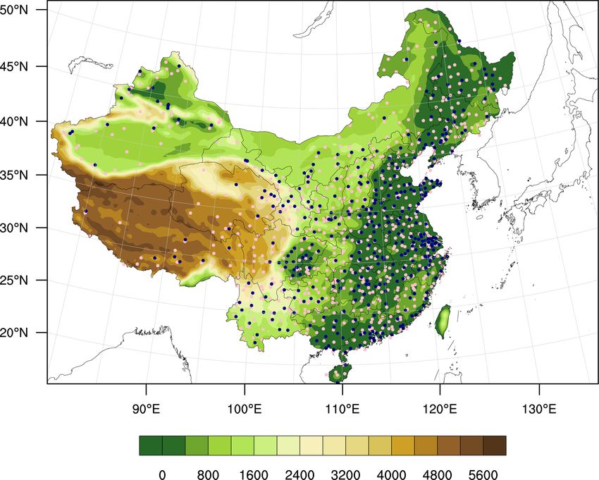
J. Zhu et al.: Effects of ozone–vegetation interactions                                                                       767

istry, biogeochemical, and biogeophysical cycles, Sadiq et         damage to vegetation, changes in meteorology in China due
al. (2017) estimated that surface O3 is 4–6 ppb higher in Eu-      to O3 –vegetation coupling, and the subsequent feedback ef-
rope, North America, and China in simulations with O3 –            fects onto O3 concentration itself are examined, which is cru-
vegetation coupling comparing the surface O3 concentra-            cial to fully understand the O3 –vegetation interactions and
tions without O3 –vegetation coupling. Based on the modi-          the following impacts on climate, biosphere, and air quality
fied Weather Research and Forecasting model with chem-             in areas with both high O3 concentrations and high vegeta-
istry (WRF-Chem), Li et al. (2016, 2018) investigated the          tion coverage.
effect of O3 exposure on hydroclimate and crop productivity
in the US and highlighted O3 damage effects on meteoro-
                                                                   2     Methods
logical fields and surface energy balance as well as the crop
yields, but the feedbacks of changing meteorology onto sur-        2.1    WRF-Chem model setup
face O3 were not investigated. Arnold et al. (2018) examined
the global climate response to O3 exposure and found O3            The WRF model is a state-of-the-art mesoscale nonhydro-
damage on vegetation can induce widespread surface warm-           static meteorological model. An atmospheric chemistry mod-
ing and changes in clouds, which could be critical on regional     ule that includes various gas-phase chemistry and aerosol
scales. Although the interactions between O3 and vegeta-           mechanisms has been implemented into and fully coupled
tion are critical to our environment, adequate representation      with WRF to create the WRF-Chem model (Grell et al.,
of O3 –vegetation interactions is still missing in most atmo-      2005; Fast et al., 2006). In WRF-Chem, both the air qual-
spheric models used for climate and atmospheric chemistry          ity and meteorological components use the same transport
simulations, at least in part due to incomplete coupling ca-       scheme, model grid, subgrid-scale transport physics, and
pacities with land surface or biospheric model components          time step. WRF-Chem has been widely used in previous
at high resolutions and in part due to limited observations to     air quality studies (e.g., Li et al., 2016, 2018; Liu et al.,
optimize O3 damage schemes for wider regional applicabil-          2018, 2020). In this study, we applied our revised WRF-
ity.                                                               Chem model based on version 3.8.1 to simulate meteoro-
   With the rapid urbanization and industrialization in the re-    logical fields and O3 concentration over China. Simulations
cent decades, China has experienced increasingly severe O3         are conducted from 24 May to 1 September every year from
pollution, which is expected to continue to worsen in the near     2014 to 2017 and the days in May were discarded as spin-up.
future. O3 concentration in China has been observed to ex-         For the land surface component within WRF, we used Noah-
ceed ambient air quality standard by 100 %–200 % (Wang et          MP, which will be described in the next subsection.
al., 2017), with the maximum 8 h mean concentration of O3             The model domain was configured at a horizontal resolu-
(MDA8 O3 ) increasing by 4.6 % per year from 2015 to 2017          tion of 27 km on the Lambert conformal projection, centered
(Silver et al., 2018). Lu et al. (2019) showed that urban sur-     at 37◦ N, 108.1◦ E, and covering all of China. The model
face O3 in China during 2013–2017 was significantly higher         has 26 vertical layers, with the lowest layer at 0.17 km and
than that in other regions around the world, and thus vegeta-      the highest layer at 17.67 km. The meteorological initial and
tion exposure to O3 is also higher in China. Li et al. (2019)      boundary conditions are provided by the 6-hourly Final Op-
also revealed the increasing trend of O3 in megacity clusters      erational Global Analysis (FNL) dataset at a horizontal res-
of China during 2013–2017, which is closely related to mete-       olution of 1◦ × 1◦ . The chemical initial and boundary condi-
orology, anthropogenic emissions, and PM2.5 concentrations.        tions were generated from the Model for Ozone and Related
Global-scale studies have highlighted China as a hotspot of        Chemical Tracer version 4 (MOZART-4), which is available
O3 pollution and damage to vegetation compared with other          at a horizontal resolution of 1.9◦ ×2.5◦ with 56 vertical layers
regions (Sadiq et al., 2017; Arnold et al., 2018; Lei et al.,      (Emmons et al., 2010).
2020). However, a comprehensive study of how O3 affects               Anthropogenic emissions were from the Multi-resolution
meteorology and air quality through O3 –vegetation interac-        Emission Inventory for China (MEIC) compiled at a spa-
tions in China at high spatial resolutions, especially under       tial resolution of 27 km and a 1-hourly temporal resolution
severe O3 pollution, is still limited but highly needed. More-     suitable for our research domain. Biogenic emissions were
over, there have been limited studies focusing on the feed-        calculated online by the Model of Emissions of Gases and
backs of O3 –vegetation coupling on O3 concentration itself,       Aerosol from Nature (MEGAN) (Guenther et al., 2006).
especially in China, which is one of the main scopes of our        Biomass burning emissions were extracted from the Fire In-
study.                                                             ventory from NCAR (FINN) version 1.5 datasets (Wiedin-
   This study, therefore, first adopted and implemented a          myer et al., 2011). Dust emissions were generated online
semi-mechanistic O3 damage scheme in a widely used re-             by the Goddard Global Ozone Chemistry Aerosol Radiation
gional atmosphere–land modeling framework and hence                and Transport model (GOCART; Ginoux et al., 2001). Gas-
used it to simulate and assess the impacts of O3 –vegetation       phase chemistry was simulated with second generation Re-
interactions on boundary-layer meteorology and air quality         gional Acid Deposition Model (RADM2; Stockwell et al.,
in China at a high spatial resolution. Specifically, O3 -induced   1990) mechanism, and the Modal Aerosol Dynamics Model

https://doi.org/10.5194/acp-22-765-2022                                              Atmos. Chem. Phys., 22, 765–782, 2022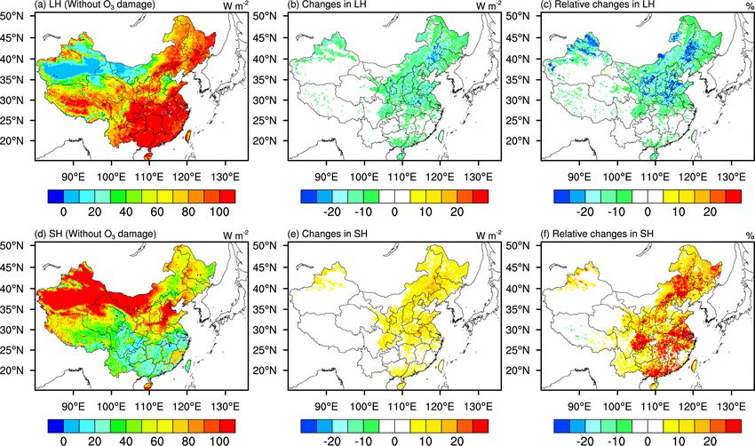
768                                                                       J. Zhu et al.: Effects of ozone–vegetation interactions

for Europe (MADE; Ackermann et al., 1998), which is cou-           2.3    O3 damage parameterization
pled with the Secondary Organic Aerosol Model (SORGAM;
                                                                   In Noah-MP, the Farquhar model (Farquhar et al., 1980) was
Schell et al., 2001) for aerosol treatment. Detailed physics
                                                                   used to calculate photosynthetic rate, whereas Ball–Berry
schemes used in the simulations are shown in Table S1 in the
                                                                   model was used to calculate stomatal conductance (Ball et
Supplement.
                                                                   al., 1987). The photosynthesis rate, A (µmol CO2 m−2 s−1 ),
                                                                   is calculated separately for sunlit and shaded leaves and is
2.2   Description of the Noah-MP model                             limited by either one of three limiting factors and can be cal-
Noah-MP is a land surface model that uses multiple options         culated as
for key land–atmosphere interaction processes (Niu et al.,
                                                                   A = min Wc , Wj , We Igs ,                                  (1)
2011). Noah-MP contains a separate vegetation canopy de-
fined by a canopy top and bottom, crown radius, and leaves         where Wc is the RuBisCO-limited photosynthesis rate, Wj is
with prescribed dimensions, orientation, density, and radio-       the light-limited photosynthesis rate, and We is the export-
metric properties. The canopy employs a two-stream radia-          limited photosynthesis rate. Igs is the growing season index
tion transfer approach along with shading effects necessary        with values ranging from 0 to 1. Stomatal conductance (gs ) is
to achieve proper surface energy and water transfer processes      computed based on the photosynthesis rate from the Farquhar
(Dickinson, 1983). Noah-MP is capable of distinguishing            model as
between C3 and C4 photosynthesis pathways and defines                     1     A es
vegetation-specific parameters for plant photosynthesis and        gs =      =m       Patm + b,                               (2)
                                                                          rs    cs ei
respiration.
   Noah-MP is available for prognostic vegetation growth           where gs is the leaf stomatal conductance (µmol m−2 s−1 ); rs
that combines a Ball–Berry photosynthesis-based stomatal           is the leaf stomatal resistance (s m2 µmol−1 ); m is an empir-
resistance (Farquhar et al., 1980; Ball et al., 1987) that allo-   ical parameter that relates stomatal conductance and photo-
cates carbon to various parts of vegetation (leaf, stem, wood,     synthesis with values ranging from 5 to 9; A is the photo-
and root) and soil carbon pools (fast and slow). GPP, LAI,         synthesis rate as described above; cs is the CO2 partial pres-
and canopy height are then predicted downstream from pho-          sure at the leaf surface (Pa); es is the vapor pressure at the
tosynthesis. Noah-MP also considers the photosynthesis of          leaf surface (Pa); ei is the saturation vapor pressure inside
sunlit and shaded leaves separately, whereby sunlit leaves are     the leaf (Pa); Patm is the atmospheric pressure (Pa); and b is
more limited by CO2 concentration while shaded leaves are          the minimum stomatal conductance.
more constrained by insolation, which may thus have differ-           As mentioned above, following Lombardozzi et al. (2015),
ent responses to O3 damage. The dynamic LAI and canopy             an O3 damage scheme was implemented in Noah-MP em-
height calculation will further affect surface energy fluxes,      bedded in WRF-Chem model version 3.8.1. The photosyn-
which will then affect the boundary-layer meteorology when         thesis rate and stomatal conductance are modified indepen-
coupling with the atmosphere model in WRF-Chem. The                dently using two sets of O3 impact factors, FpO3 and FcO3 ,
land use types and the vegetation parameters are based on          respectively, which are then multiplied to the initial A and gs
the US Geological Survey (USGS) embedded in Noah-MP.               calculated by the Farquhar–Ball–Berry model, respectively.
Figure 1 shows the spatial distribution of vegetation frac-        Lombardozzi et al. (2012) found that independently modi-
tion of dominant vegetation types in China. The distributions      fying stomatal conductance and photosynthesis can improve
of main vegetation groups (broadleaf, needleleaf, crop, and        the model prediction of plant response to O3 damage. The
grass) that have different sensitivities to O3 damage follow-      two damage factors are calculated based on the cumulative
ing Lombardozzi et al. (2015) are shown in Fig. 1.                 uptake of O3 (CUO), which integrates the O3 flux inside
   In this study, the O3 concentration simulated by the chem-      leaves through the stomata throughout the growing season.
ical module of the WRF-Chem model was also dynamically             The CUO (mmol m−2 ) is calculated as
passed onto the Noah-MP land surface model at every time                          X         [O3 ]
step to modify the photosynthesis and stomatal conductance         CUO = 10−6                          1t,                     (3)
                                                                                      kO3 rs + ra + rb
due to O3 damage. The land surface variables simulated by
Noah-MP were also dynamically passed back onto the at-             where [O3 ] is the surface O3 concentration (nmol m−3 );
mospheric components, thus allowing immediate, two-way             kO3 = 1.61 is the ratio of leaf resistance to O3 to leaf re-
feedback effects onto meteorological fields, O3 , and other at-    sistance to water (Uddling et al., 2012); rs is the stom-
mospheric chemical constituents. In this way, land surface         atal resistance, ra is the aerodynamic resistance and rb is
processes, atmospheric dynamics, and atmospheric chem-             the boundary-layer resistance (s m−1 ); 1t is the model time
istry in the WRF-Chem model were fully coupled.                    step (s). CUO is only accumulated when LAI is larger
                                                                   than 0.4 and O3 flux is larger than a threshold value of
                                                                   0.8 nmol O3 m−2 s−1 to consider the detoxification effect of
                                                                   plants to O3 damage.

Atmos. Chem. Phys., 22, 765–782, 2022                                                  https://doi.org/10.5194/acp-22-765-2022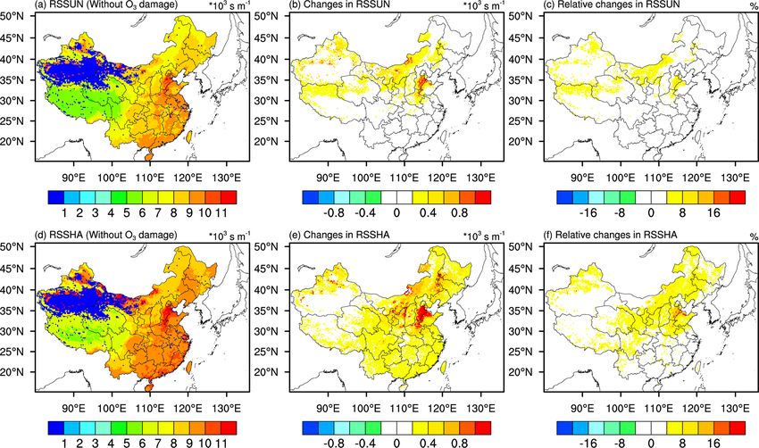
J. Zhu et al.: Effects of ozone–vegetation interactions                                                                                       769

Figure 1. The vegetation fraction of (a) broadleaf, (b) needleleaf, (c) cropland, (d) grass, (e) others, and (f) dominant vegetation types.

 The two damage factors have linear relationships with                    be attributed to O3 –vegetation interactions. In this work, each
CUO and can be calculated as follows:                                     simulation was conducted from 24 May to 1 September ev-
                                                                          ery year from 2014 to 2017 and the days in May was dis-
FpO3 = ap × CUO + bp                                             (4)      carded as spin-up. For each simulation in the 4 years, an-
FcO3 = ac × CUO + bc ,                                           (5)      thropogenic emissions were kept at 2014 levels, while mete-
                                                                          orological fields were changing every year. The 4-year June–
where FpO3 is the O3 damage factor for photosynthesis and                 July–August (JJA) averaged results were analyzed and com-
FcO3 is the O3 damage factor for stomatal conductance; ap ,               pared. JJA was selected because of the most severe O3 pollu-
bp , ac , and bc are empirical slopes and intercepts of three             tion in this season and because it is within the active growing
different plant groups (broadleaf trees, needleleaf trees, and            season of the plants.
grasses or crops) from Lombardozzi et al. (2015). The val-                   The simulated meteorological variables and air pollutant
ues of these slopes and intercepts are shown in Table 1. The              concentrations were evaluated using available in situ obser-
original photosynthesis and stomatal conductance are then                 vations in China. The daily meteorological observations in-
multiplied by the two damage factors, respectively, to get the            cluding temperature at 2 m (T2 m ), relative humidity at 2 m
modified photosynthesis and stomatal conductance under O3                 (RH2 m ), and wind speed at 10 m (WS10 m ) above displace-
exposure.                                                                 ment height were from the National Meteorological Infor-
                                                                          mation Center. There are 698 stations in the study domain.
2.4   Model experiments and evaluation                                    The air pollutant observations were provided by the China
                                                                          National Environmental Monitoring Center (CNEMC) net-
Two sets of experiments were conducted in this study.
                                                                          work, which offers hourly concentrations of particulate mat-
We performed a control simulation (simu_withoutO3 ) with-
                                                                          ter with an aerodynamic diameter of less than 2.5 µm (PM2.5 )
out O3 damage on vegetation and a production simulation
                                                                          and 10 µm (PM10 ), carbon monoxide (CO), O3 , sulfur diox-
(simu_withO3 ) with O3 damage on vegetation. Detailed in-
                                                                          ide (SO2 ), and nitrogen dioxide (NO2 ). The locations of
formation of the experiments is shown in Table 2. In the
                                                                          meteorological stations and the sites of CNEMC network
simu_withO3 experiment, the O3 concentration simulated by
                                                                          are shown in Fig. 2. The statistical parameters including
the chemical module of the model is dynamically passed onto
                                                                          mean values (mean) of observations and simulated variables,
the land surface model at every time step to modify the pho-
                                                                          their standard deviations (SDs), indices of agreement (IOAs),
tosynthesis and stomatal conductance. The differences be-
                                                                          mean biases (MBs), and correlation coefficients (CORRs)
tween the two sets of experiments including vegetation phys-
iology, meteorological fields, and O3 concentration can thus

https://doi.org/10.5194/acp-22-765-2022                                                        Atmos. Chem. Phys., 22, 765–782, 2022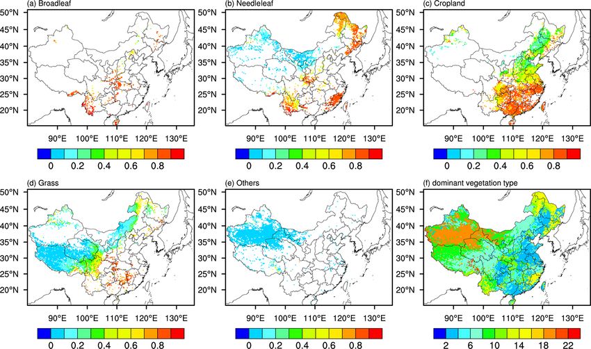
770                                                                            J. Zhu et al.: Effects of ozone–vegetation interactions

Table 1. Slopes (per mmol m−2 ) and intercepts (unitless) used for O3 damage factors in Eqs. (4) and (5), following Lombardozzi et al. (2015).

                                                          Photosynthesis                   Conductance
                                                    Slope (ap )   Intercept (bp )   Slope (ac )   Intercept (bc )
                              Broadleaf               0.0000             0.8752         0.0000           0.9125
                              Needleleaf              0.0000             0.8390         0.0048           0.7823
                              Grasses and crops      −0.0009             0.8021         0.0000           0.7511

Table 2. Description of the two sets of model experiments. ICs are initial conditions; BCs are boundary conditions.

                               Experiment name            Year          Anthropogenic      Meteorological ICs
                                                                        emission           and BCs
                               simu_withoutO3       2014–2017 JJA       Year 2014          FNL
                               simu_withO3          2014–2017 JJA       Year 2014          FNL

                                                                         values ranging from 4.38 in the year 2014 to 7.33 in the year
                                                                         2016, but the CORR values with observations are still high
                                                                         (CORR > 0.7). Wind speed is also overestimated by more
                                                                         than 0.38 m s−1 , which might be caused by the underesti-
                                                                         mation of terrain height as reported in other WRF model-
                                                                         ing studies (Brunner et al., 2015; Liu et al., 2020). The de-
                                                                         tailed evaluation results for each city and for seven major ge-
                                                                         ographic regions of China are shown in Tables S5–S10. The
                                                                         classification of the geographic regions is shown in Fig. S2.
                                                                         As shown in these tables, the model can reasonably capture
                                                                         the spatial distribution of these meteorological variables. For
                                                                         example, the larger values of T2 m and RH2 m in cities from
                                                                         southern China compared with the cities in northern China
                                                                         (Table 4) can be reasonably simulated. We also found that
                                                                         the model simulations have better performance in northeast-
                                                                         ern China, central China, and southern China in terms of IOA
                                                                         and CORR as shown in these tables (Table 4).
Figure 2. Site locations of air quality monitoring sites (blue dots)        Table 5 shows the city-averaged evaluation results of six
and the meteorological monitoring sites (pink dots), and terrain         air pollutants simulated from the modified model. The infor-
height (m) shown by the color contours.
                                                                         mation of the major cities used for air pollutant evaluation
                                                                         is shown in Table S11. Form Table 5, positive MB values
were computed to evaluate the model performance in this                  for O3 , PM2.5 , SO2 , and NO2 , and negative MB values for
study.                                                                   CO are found. The overestimation of O3 by WRF-Chem was
                                                                         also reported by Hu et al. (2016) and Gao et al. (2020). For
                                                                         PM10 , both positive and negative MB values are found for
3     Results                                                            different years. The results indicate general overestimation
                                                                         by the model of most air pollutants except for CO. The un-
3.1    Model evaluation                                                  derestimation of CO can be explained by either O3 chem-
Table 3 shows the city-averaged evaluation results of me-                istry, which points to the problem related to low titration, or
teorological variables from the modified model. The infor-               in the underestimation of dry deposition by the model, which
mation of the major cities used for evaluation is shown in               is also affected by the modification of the model. The IOA
Table S4. From Table 3, we can find that T2 m is underes-                of air pollutant concentration ranges from 0.36 (SO2 ) to 0.63
timated with MB values ranging from −1.00 ◦ C in 2017 to                 (O3 ). The correlation coefficient of air pollutants ranges from
−0.70 ◦ C in 2014. The IOA and CORR are generally higher                 0.14 (PM10 ) to 0.66 (O3 ). Detailed evaluation results for each
than 0.8, indicating that the model could reasonably simu-               city and major geographic regions of China are shown in Ta-
late the variations of T2 m . Unlike temperature, relative hu-           bles S9–S14 and Table 6. In terms of the evaluation for O3 ,
midity is overestimated by the model simulations with MB                 the model has better performance in northeastern China, east-

Atmos. Chem. Phys., 22, 765–782, 2022                                                         https://doi.org/10.5194/acp-22-765-2022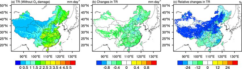
J. Zhu et al.: Effects of ozone–vegetation interactions                                                                                     771

Table 3. Evaluation results for the temperature at 2 m (T2 m ), relative humidity at 2 m (RH2 m ), and wind speed at 10 m (WS10 m ) for different
years in China. Mean_obs (Mean_simu) is the mean value of observation (model simulation); SD_obs (SD_simu) is the standard deviation
of the observation (model simulation); IOA is the index of agreement; CORR is the correlation coefficient; MB is the mean bias.

                                       Year    Mean_obs    SD_obs    Mean_simu     SD_simu     IOA    CORR       MB
                           T2 m       2014        25.41      2.61         24.71        2.27    0.86     0.87    −0.70
                           (◦ C)      2015        25.41      2.56         24.67        2.24    0.86     0.89    −0.74
                                      2016        26.35      2.82         25.44        2.61    0.85     0.85    −0.91
                                      2017        26.29      3.17         25.28        3.16    0.81     0.78    −1.00
                           RH2 m      2014        74.77     10.22         79.14        8.96    0.67     0.71     4.38
                           (%)        2015        73.34     10.75         80.50        8.73    0.68     0.75     7.16
                                      2016        74.14     10.81         81.47       10.10    0.70     0.73     7.33
                                      2017        73.24     11.65         79.89        9.62    0.68     0.69     6.63
                           WS10 m     2014         1.84      0.66          2.22        1.16    0.54     0.40     0.38
                           (m s−1 )   2015         2.00      0.74          2.48        1.35    0.55     0.44     0.48
                                      2016         1.99      0.70          2.47        1.32    0.54     0.45     0.48
                                      2017         2.02      0.72          2.51        1.42    0.53     0.45     0.50

Table 4. Evaluation results of temperature at 2 m (T2 m ), relative humidity at 2 m (RH2 m ), and wind speed at 10 m (WS10 m ) in seven major
geographic regions from the implemented model. NEC is northeast China, NC is north China, CC is central China, EC is east China, SC
is south China, SWC indicates southwest China, and NWC is northwest China. Mean_obs (Mean_simu) is the mean value of observations
(model simulations); SD_obs (SD_simu) is the standard deviation of the observations (model simulations); IOA is the index of agreement;
CORR is the correlation coefficient; MB is the mean bias.

                                      Region   Mean_obs    SD_obs    Mean_simu     SD_simu      IOA   CORR        MB
                          T2 m        NEC          23.01      3.05         22.73        3.01   0.94      0.91   −0.28
                          (◦ C)       NC           24.94      2.76         25.84        2.84   0.86      0.88    0.88
                                      CC           27.62      3.05         26.87        2.75   0.92      0.88   −0.75
                                      EC           27.33      2.99         26.46        2.58   0.90      0.89   −0.87
                                      SC           28.60      1.49         28.61        1.30   0.75      0.64    0.01
                                      SWC          23.20      2.32         21.61        2.14   0.77      0.80   −1.58
                                      NWC          20.20      2.87         18.55        3.01   0.77      0.89   −1.65
                          RH2 m       NEC          71.70     11.49         71.98       14.00   0.85      0.79    0.93
                          (%)         NC           63.25     13.94         57.01       14.08   0.79      0.75   −6.24
                                      CC           79.23     10.11         88.29        8.61   0.70      0.71    9.06
                                      EC           78.93      9.99         88.80        8.31   0.69      0.79    9.87
                                      SC           81.26      6.54         88.41        5.66   0.62      0.60    7.14
                                      SWC          78.92      9.11         93.34        5.13   0.52      0.64   13.40
                                      NWC          57.93     13.34         58.48       14.10   0.75      0.76    0.55
                          WS10 m      NEC           2.22      0.93          3.08        1.80   0.62      0.62     0.86
                          (m s−1 )    NC            2.06      0.72          2.45        1.29   0.57      0.48     0.38
                                      CC            2.06      0.81          2.38        1.41   0.61      0.51     0.33
                                      EC            2.18      0.76          2.85        1.54   0.59      0.55     0.67
                                      SC            2.02      0.76          2.81        1.51   0.52      0.43     0.80
                                      SWC           2.16      0.76          2.54        1.40   0.57      0.51     0.37
                                      NWC           1.46      0.50          2.91        1.38   0.30      0.23     1.45

ern and southern China, which may suffer the most severe O3                pared the evaluation results between the original model and
damage. Our results are generally consistent with the evalu-               the modified model, as shown in Tables S2 and S3 in the Sup-
ation results of the Community Multiscale Air Quality Mod-                 plement and Tables 3 and 5 here. We found no obvious dif-
eling (CMAQ) simulation over China by Liu et al. (2020).                   ferences in the evaluation results between the original model
MBs of SO2 , NO2 , and CO are consistent in both magni-                    results and the revised model results. It should be noted that
tude and sign with Liu et al. (2020), while the MBs of PM                  this study might not be able to and was not meant to improve
and O3 are larger than Liu et al. (2020). Correlation coeffi-              model accuracy, but our modified model is able to capture
cients of air pollutants are also of similar magnitude with Liu            O3 –vegetation interactions without worsening model perfor-
et al. (2020), showing that our model results can well cap-                mance. Overall, there are systematic biases in simulated vari-
ture the temporal variations of air pollutants. We also com-               ables especially the air pollutant concentrations, but the spa-

https://doi.org/10.5194/acp-22-765-2022                                                         Atmos. Chem. Phys., 22, 765–782, 2022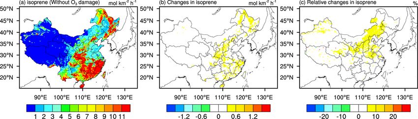
772                                                                     J. Zhu et al.: Effects of ozone–vegetation interactions

tial distributions of both meteorological variables and air pol-   sponse to the PSN reductions, LAI and GPP also decrease.
lutant concentrations are reasonably simulated by the model,       More than 0.4 reductions in LAI are found in central and
lending trust to the use of the model for sensitivity studies      northern China (Fig. 4e), corresponding to more than 20 %
to examine the effects of O3 –vegetation interactions on the       reductions in LAI; in other regions, 5 %–15 % reductions
atmospheric environment.                                           in LAI are observed. More than 0.8 g C m−2 d−1 reductions
                                                                   in GPP are found generally in China. Similar to Fig. 3c,
3.2   Responses of vegetation to O3 damage
                                                                   we find that GPP decreases by ∼ 20 % in northeastern and
                                                                   southern China and decreases by more than 40 % in other
O3 can adversely affect photosynthesis rate and stomatal con-      regions (Fig. 4i). Based on offline models without consider-
ductance and therefore interfere with vegetation growth, pro-      ing atmosphere–biosphere coupling, O3 damage was found
ductivity, and transpiration. To understand the O3 -induced        to decrease GPP at most by 11 %–17 % in the east coast
damage on vegetation physiology, the spatial distribution,         hotspots of the US (Yue and Unger, 2014). Using the of-
and changes in stomatal resistance (RS), photosynthesis rate       fline CLM model, Lombardozzi et al. (2015) estimated that
(PSN), LAI, GPP, and transpiration rate (TR) during 2014–          the present O3 exposure reduces GPP globally by 8 %–12 %.
2017 summer (June–July–August) were analyzed.                      Based on the Regional Climate-Chemistry Model version 4
   Figure 3a and d display the spatial distribution of sun-        (RegCM-CHEM4) model coupled with Yale Interactive ter-
lit stomatal resistance (RSSUN) and shaded stomatal resis-         restrial Biosphere (YIBs) model, Xie et al. (2019) revealed
tance (RSSHA) from the simu_withoutO3 experiment, re-              that O3 damage induces a significant reduction (12.1±4.4 %)
spectively. The absolute and relative changes in RSSUN             in the GPP, up to 35 % in summer over China (Table S15).
(RSSHA) between simu_withO3 and simu_withoutO3 exper-              Comparing our results with previous studies, our results are
iments are shown in the middle and the right panel of Fig. 3,      broadly consistent with Xie et al. (2019), but the magnitude
separately. In general, simulated stomatal resistance in east-     is larger than the studies conducted by Yue and Unger (2014)
ern China is larger than that in western China. Both RSSUN         and Lombardozzi et al. (2015). Differences or uncertainties
and the RSSHA are enhanced in response to O3 damage to             may arise from the different model settings. It appears that
vegetation. The maximum increases in RSSUN and RSSHA               offline models as used by Yue and Unger (2014) and Lombar-
can be up to 1.0×10³ s m−1 , which is equivalent to a ∼ 16 %       dozzi et al. (2015) generally found smaller damage than stud-
increase compared to the simu_withoutO3 simulation. Com-           ies with two-way coupling between the atmosphere and bio-
paring the changes in RSSUN vs. RSSHA, the changes in              sphere as used by Xie et al. (2019) and our work; this could
RSSHA are larger than that in RSSUN, reflecting the larger         be due to the existence of positive biosphere–atmosphere
sensitivity of shaded leaves to O3 damage (Kinose et al.,          feedbacks that potentially worsen O3 damage, as will be dis-
2017). Northern China experiences larger changes in stom-          cussed in subsequent sections. Different O3 damage schemes
atal resistance generally, especially in the Henan, Hebei, and     employed in the models may also be a source of differences,
Shandong provinces, where the changes in stomatal resis-           although we note that both this work and Lombardozzi et
tance are twice as large as the changes in stomatal resistance     al. (2015) used the same scheme, so the differences appear to
over other regions.                                                arise more likely from the effect of coupling and other model
   The spatial distribution of 2014–2017 JJA mean PSN,             settings than from the schemes alone.
LAI, and GPP from the simu_withoutO3 simulations and                  The spatial distributions of dominant vegetation types in
their changes induced by O3 damage are presented in Fig. 4.        China are shown in Fig. 1, where we can see that the crop-
From Fig. 4a, we find that the PSN values are generally            lands dominant in eastern China and especially in southern
higher in eastern China compared with western China with           China suffer the greatest GPP reductions, indicating that crop
the largest values of up to ∼ 7 µmol CO−1  2 m
                                                −2 s−1 . Similar   yields in China would also be heavily affected by O3 damage.
spatial distribution and hotspot areas can also be observed for       Figure 5 depicts the spatial distribution of transpiration
LAI (Fig. 4d) and GPP (Fig. 4g), with LAI and GPP values           rate (TR) of vegetation and the changes in transpiration rate
in hotspot areas up to 3.6 and 10 g C m−2 d−1 , respectively.      induced by O3 damage. TR values are higher in eastern
We also find that the Henan, Hebei, Shanxi, and Shandong           China, where there is larger vegetation coverage (Fig. 5a).
provinces have smaller values of PSN, LAI, and GPP when            As shown in Fig. 5b, TR deceases by 0.2–1.0 mm d−1 gener-
compared with other provinces in eastern China.                    ally in eastern China with large reductions in northern China,
   With O3 damage, PSN decreases in general, with absolute         especially in the Henan, Shandong, Anhui, and Jiangsu
changes in PSN ranging from 0.6 to 3.6 µmol CO2−1 m−2 s−1          provinces. In terms of relative changes, TR decreases by
(Fig. 4b), representing 20 %–40 % reductions in PSN. For           ∼ 12 % in northeastern and southern China, while more than
northeastern and southern China, where the original PSN val-       24 % reductions are found in other regions. Transpiration is
ues are large, ∼ 20 % reductions in PSN are found (Fig. 4c).       affected by the changes in both RS and LAI. With O3 dam-
In western China where the dominant vegetation type is             age, both the increases in RS (Fig. 3c and f) and decreases
grassland and the original PSN values are small, more than         in LAI (Fig. 4f) cause TR to decrease, as shown in Fig. 5b
40 % of PSN is reduced due to O3 damage (Fig. 4c). In re-          and c. Comparing the changes in RS (Fig. 3c and f), LAI

Atmos. Chem. Phys., 22, 765–782, 2022                                                https://doi.org/10.5194/acp-22-765-2022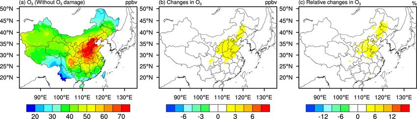
J. Zhu et al.: Effects of ozone–vegetation interactions 773
Table 5. Evaluation results for the air pollutants in China. Mean_obs (Mean_simu) is the mean value of observation (model simulation);
SD_obs (SD_simu) is the standard deviation of the observation (model simulation); IOA is the index of agreement; CORR is the correlation
coefficient; MB is the mean bias.
Year Mean_obs SD_obs Mean_simu SD_simu IOA CORR MB
O3 2014 29.79 9.95 51.49 18.60 0.48 0.57 22.13
(ppb) 2015 32.04 10.16 48.98 18.27 0.54 0.55 16.95
2016 33.28 10.59 48.47 18.18 0.56 0.58 15.14
2017 35.74 11.71 49.50 19.61 0.63 0.66 13.82
PM2.5 2014 46.30 21.52 63.28 27.15 0.52 0.33 18.61
(µg m−3 ) 2015 38.52 17.30 55.56 24.85 0.55 0.42 16.66
2016 31.86 13.96 56.70 25.69 0.47 0.40 24.54
2017 28.82 12.23 56.34 25.70 0.40 0.30 27.65
PM10 2014 80.79 31.62 71.74 28.65 0.47 0.22 −7.51
(µg m−3 ) 2015 72.03 29.74 63.83 26.29 0.50 0.26 −8.93
2016 59.68 22.21 65.01 27.29 0.49 0.24 4.65
2017 57.83 22.18 64.78 27.25 0.41 0.14 6.95
SO2 2014 6.11 2.36 8.41 3.22 0.48 0.41 2.36
(ppb) 2015 4.78 1.89 8.39 3.26 0.44 0.45 3.64
2016 4.17 1.57 8.08 3.16 0.41 0.36 3.92
2017 3.83 1.33 8.58 3.52 0.36 0.42 4.78
NO2 2014 17.20 4.51 17.23 4.63 0.41 0.26 0.06
(ppb) 2015 16.01 4.47 17.37 4.98 0.43 0.31 1.43
2016 15.29 4.29 17.35 5.11 0.43 0.31 2.06
2017 15.83 4.37 17.84 5.12 0.43 0.32 2.02
CO 2014 0.76 0.19 0.44 0.11 0.48 0.42 −0.32
(ppm) 2015 0.67 0.15 0.45 0.11 0.49 0.42 −0.22
2016 0.65 0.14 0.45 0.11 0.50 0.45 −0.20
2017 0.64 0.12 0.46 0.11 0.47 0.38 −0.18
(Fig. 4f) and TR (Fig. 5c), we can find that the distribution of regions (Fig. 6f), indicating that O3 damage shifts the energy
changes in TR is more consistent with that of RS, reflecting balance toward more net radiation being dissipated by SH
the dominance of RS in controlling TR. flux than LH flux, with ramifications for surface temperature.
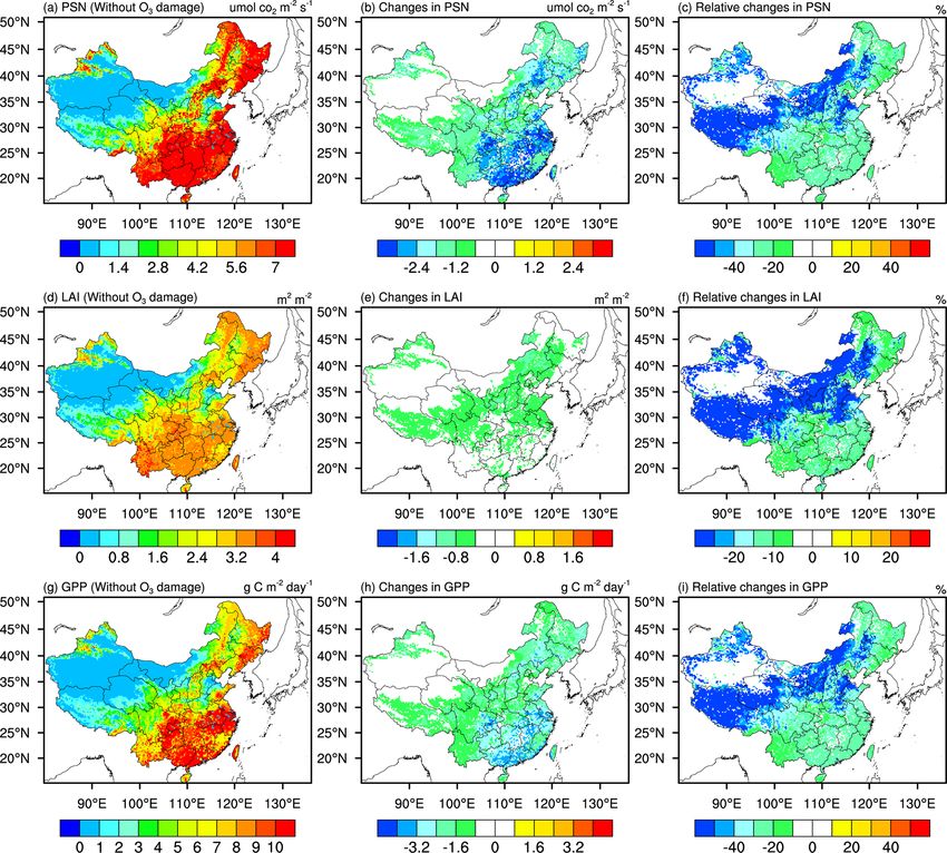
Figure 7 shows the distribution and the changes in sur-
face relative humidity, temperature and planetary boundary-
3.3 Changes in meteorology due to O3 –vegetation layer height (PBLH) in response to O3 damage. Reductions
coupling in transpiration rate can directly cause reductions in relative
humidity. As shown in Fig. 7b, relative humidity has at least
Through interacting with vegetation, O3 has the potential to
3 % absolute reductions. Values of relative humidity decrease
further affect the meteorological environment in China via
more in northern China than in southern China. Similar to the
modifying, e.g., surface heat fluxes, temperature, humidity,
changes in TR (Fig. 5b), larger reductions in relative humid-
and boundary-layer height. The distribution of meteorologi-
ity (3 %–9 %) are found over the Henan, Hebei, Shandong,
cal variables from simulations with and without O3 damage
and Anhui provinces. The decreases in LH flux and increases
is thus compared and analyzed in this section.
in SH flux following the changes in transpiration rate drive
Figure 6 shows the spatial distribution of latent heat (LH)
the increases in temperature and contribute to PBLH growth.
flux and sensible heat (SH) flux, and the changes in LH
As presented in Fig. 7e and h, the distribution and hotspot
and SH due to O3 –vegetation coupling. With O3 included
areas of the changes in temperature and PBLH are similar
in the model simulations, the LH flux decreases by more
to those in relative humidity. Generally, northern China has
than 4 W m−2 (Fig. 6b) on average following the decreases
larger increases of temperature and PBLH compared with
in transpiration rate. Hotspot areas are found in the Henan,
other regions. Generally, temperature increases by 0.2–0.8 K
Shandong, Anhui, and Jiangsu provinces, where reductions
and PBLH increases by 40–120 m for northern China. The
in LH can be up to 30 W m−2 . Meanwhile, 5–30 W m−2 in-
hotspot areas experience at least 0.6 K increases in tempera-
creases in SH flux are observed in central and northern China
ture and 80 m increases in PBLH.
(Fig. 6d). With O3 –vegetation coupling, more than 20 % re-
As shown in Table S15, our results are comparable
ductions in LH flux are found in central and northern China
with results from a regional simulation conducted by Li et
(Fig. 6c), 20 % increments in SH flux are found in similar
https://doi.org/10.5194/acp-22-765-2022 Atmos. Chem. Phys., 22, 765–782, 2022774 J. Zhu et al.: Effects of ozone–vegetation interactions
Table 6. Evaluation results of air pollutants in seven major geographic regions simulated by the implemented model. NEC is northeast
China, NC is north China, CC is central China, EC is east China, SC is south China, SWC indicates southwest China, and NWC is northwest
China. Mean_obs (Mean_simu) is the mean value of observations (model simulations); SD_obs (SD_simu) is the standard deviation of the
observations (model simulations); IOA is the index of agreement; CORR is the correlation coefficient; MB is the mean bias.
Region Mean_obs SD_obs Mean_simu SD_simu IOA CORR MB
O3 NEC 32.49 10.54 44.54 15.70 0.64 0.64 11.47
(ppb) NC 38.56 10.81 70.59 25.11 0.40 0.55 32.02
CC 31.68 11.20 57.13 18.17 0.47 0.60 26.82
EC 29.67 10.82 40.53 18.99 0.60 0.61 11.21
SC 19.90 8.40 34.21 14.68 0.53 0.64 14.90
SWC 24.27 9.12 42.07 13.19 0.47 0.50 18.80
NWC 26.63 8.12 51.65 13.70 0.34 0.42 25.58
PM2.5 NEC 42.66 25.15 43.33 19.28 0.57 0.39 −0.83
(µg m−3 ) NC 61.60 28.28 66.83 27.81 0.68 0.52 7.03
CC 52.11 30.55 94.27 39.40 0.35 0.11 45.50
EC 52.87 25.71 87.37 38.97 0.50 0.39 36.63
SC 22.58 10.16 28.62 15.17 0.67 0.57 6.92
SWC 32.82 12.22 76.69 33.49 0.27 0.08 47.55
NWC 45.27 14.54 42.80 14.07 0.39 0.03 −1.45
PM10 NEC 79.68 36.48 48.99 20.64 0.49 0.32 −32.25
(µg m−3 ) NC 111.17 39.69 74.29 29.33 0.54 0.38 −35.90
CC 84.80 41.01 107.65 41.51 0.37 0.05 26.30
EC 78.16 35.64 99.51 40.90 0.54 0.34 23.64
SC 43.64 15.72 34.11 16.14 0.58 0.47 −8.54
SWC 58.84 20.15 87.07 35.49 0.31 −0.07 32.17
NWC 88.54 28.17 47.77 14.72 0.35 −0.13 −39.68
SO2 NEC 4.91 1.95 5.10 2.55 0.60 0.42 0.27
(ppb) NC 8.69 3.52 8.12 3.20 0.54 0.40 −0.57
CC 7.34 2.09 14.56 5.45 0.36 0.47 7.23
EC 5.39 2.24 7.86 3.19 0.57 0.53 2.40
SC 3.50 0.89 4.15 1.52 0.42 0.50 0.71
SWC 4.74 1.93 15.71 5.12 0.31 0.13 11.42
NWC 6.65 2.90 4.31 1.50 0.46 0.34 −2.28
NO2 NEC 19.51 4.84 14.07 5.27 0.41 0.11 −5.66
(ppb) NC 19.57 5.13 14.05 4.14 0.48 0.27 −5.61
CC 16.75 4.32 19.70 5.57 0.38 0.32 2.83
EC 16.24 4.78 28.83 6.88 0.40 0.39 12.65
SC 13.23 3.48 14.02 3.96 0.38 0.29 1.01
SWC 17.30 3.70 20.02 4.58 0.34 0.12 3.11
NWC 16.93 4.77 8.92 2.11 0.41 0.19 −7.98
CO NEC 0.64 0.17 0.38 0.12 0.48 0.61 −0.27
(ppm) NC 0.90 0.25 0.47 0.13 0.47 0.41 −0.42
CC 0.81 0.17 0.58 0.14 0.49 0.45 −0.22
EC 0.66 0.16 0.56 0.14 0.63 0.54 −0.09
SC 0.66 0.11 0.32 0.08 0.36 0.41 −0.34
SWC 0.69 0.14 0.49 0.11 0.49 0.29 −0.19
NWC 0.89 0.25 0.25 0.04 0.35 0.18 −0.63
al. (2016), which showed that O3 damage decreases LH flux dozzi et al., 2015; Sadiq et al., 2017; Zhou et al., 2018) to
by 10–27 W m−2 and O3 damage increases temperature by represent a more conventional detoxifying effect, instead of
0.6–2.0 ◦ C in the US. However, in their study, Li et al. (2016) lowering the threshold value that would cause much larger
assumed that O3 damage to plants happens when O3 con- changes in the surface fluxes and meteorological fields. Us-
centration is over a threshold of 20 ppb to imitate a weaker ing a two-way coupling model and the same O3 damage
detoxifying effect of plants, instead of the 40 ppb threshold scheme, Arnold et al. (2018) revealed that O3 causes less than
that was commonly used in previous studies. Considering the 8 W m−2 changes in surface heat fluxes regionally, which is
severe O3 air pollution in China, we resorted to use the more smaller than the changes of surface heat fluxes in our study.
universal O3 threshold used by previous studies (Lombar- One possible reason is that the simulated changes in O3 and
Atmos. Chem. Phys., 22, 765–782, 2022 https://doi.org/10.5194/acp-22-765-2022J. Zhu et al.: Effects of ozone–vegetation interactions 775
Figure 3. Spatial distribution of mean stomatal resistance in JJA of 2014–2017 for (a) sunlit leaves (RSSUN) and (d) shaded leaves
(RSSHA) from the simu_withoutO3 experiment. Absolute changes in (b) RSSUN and (e) RSSHA caused by O3 damage. Relative changes in
(c) RSSUN and (f) RSSHA caused by O3 damage. Absolute changes are the RSSUN (RSSHA) from simu_withO3 minus RSSUN (RSSHA)
from simu_withoutO3 . Relative changes are calculated by absolute changes over the RSSUN (RSSHA) from simu_withoutO3 .
aerosol in Arnold et al. (2018) did not feed back onto radia- stance, by incorporating O3 –LAI coupling in chemical trans-
tion and climate simulation or affect LAI. port model, Zhou et al. (2018) found an O3 feedback of
−1.8 to +3 ppb globally. Another similar work conducted
by Gong et al. (2020) showed that O3 -induced inhibition in
3.4 O3 –vegetation feedbacks on O3 concentrations
stomatal conductance increases surface O3 by 2.1 ppb in east-
O3 -induced changes in vegetation, surface fluxes, and the ern China, while considering the addition effects of O3 on
overlying meteorology can also constitute important feed- isoprene emission slightly reduces surface O3 concentrations
back effects onto O3 concentration itself. Figure 8 shows the by influencing the precursors. Soil moisture deficit, which
spatial distribution of surface O3 concentration. The change has been shown to reduce stomatal uptake, if considered, will
in surface O3 concentration during daytime is also shown also contribute to the enhancement in O3 concentration (Ryd-
in Fig. S2. As shown in Fig. 8a (Fig. S2), surface O3 con- saa et al., 2016). Together with previous findings, it is in-
centration is higher in central and northern China during creasingly clear that meteorological feedback could be an im-
summer. In terms of the feedbacks on O3 concentration, portant pathway whereby O3 –vegetation interactions can fur-
we found generally enhancements in O3 concentration when ther worsen O3 air quality, almost doubling the effect of bio-
O3 –vegetation interactions are accounted for, thus represent- geochemical feedback alone (i.e., via changes in O3 -relevant
ing a positive feedback that worsens O3 air quality (Fig. 8b). chemical fluxes alone). It should be cautiously noted that in
O3 concentration increases the most (by up to 6 %) in the terms of magnitude alone the model biases in O3 are com-
Hebei, Shanxi, and Henan provinces, with the maximum in- parable and sometimes larger than the up to 6 ppb systematic
crement of 6 ppb. The enhancement in surface O3 concentra- enhancement caused by O3 damage, which represents be one
tion from our study is at a similar magnitude to that from the major source of uncertainties in our study.
study conducted by Sadiq et al. (2017), in which both biogeo- Reduced dry deposition due to stomatal closure and re-
chemical and meteorological feedbacks from O3 –vegetation duced LAI, as well as increased isoprene emission, are all
interactions to O3 are considered. Without considering the found to be the drivers for the overall positive O3 feedback.
meteorological feedbacks following the changes in transpi- Reductions in dry deposition velocity, following closely the
ration to O3 concentrations, smaller feedbacks on surface O3 corresponding reductions in transpiration rate as both pro-
concentrations are found by the following studies. For in- cesses are modulated by stomatal regulation, contribute in
https://doi.org/10.5194/acp-22-765-2022 Atmos. Chem. Phys., 22, 765–782, 2022776 J. Zhu et al.: Effects of ozone–vegetation interactions Figure 4. Spatial distribution of 2014–2017 JJA mean (a) photosynthesis rate (PSN), (d) leaf area index (LAI), and (g) gross primary productivity (GPP) from the simu_withoutO3 experiment; absolute changes in (b) PSN, (e) LAI, and (h) GPP caused by O3 damage; and relative changes in (c) PSN, (f) LAI, and (i) GPP caused by O3 damage. Absolute changes are the results from simu_withO3 minus results from simu_withoutO3 . Relative changes are calculated from the absolute changes over the results from simu_withoutO3 . Figure 5. Spatial distribution of 2014–2017 JJA mean (a) transpiration rate (TR), and (b) absolute changes and (c) relative changes in TR caused by O3 damage. Atmos. Chem. Phys., 22, 765–782, 2022 https://doi.org/10.5194/acp-22-765-2022
J. Zhu et al.: Effects of ozone–vegetation interactions                                                                           777

Figure 6. Spatial distribution of mean (a) latent heat flux (LH) and (d) sensitive heat flux (SH) from the simu_withoutO3 experiment;
absolute changes in (b) LH flux and (e) SH flux in JJA of 2014–2017 caused by O3 damage; and relative changes in (c) LH flux and (f) SH
flux caused by O3 damage. Absolute changes are the LH (SH) flux from simu_withO3 minus LH (SH) flux simu_withoutO3 . Relative
changes are calculated by absolute changes over LH (SH) flux from simu_withoutO3 .

part to the O3 enhancement. Figure 9 shows the spatial distri-        sulting damage on vegetation and crops, but the feedback ef-
bution of isoprene emission and its changes due to O3 dam-            fects onto air quality and climate have not been fully charac-
age. We observe general increases in isoprene emission in             terized. Previous studies mainly focused on the global scale
eastern China, mainly due to increased surface temperature            with coarse spatial resolutions, which did not fully capture
(Fig. 7e and f) that is more than enough to offset reduced            the spatial distribution of O3 damage on vegetation in China.
isoprene caused by reduced LAI (Fig. 4e and f). All in all,           Based on the results from global studies pointing out that
O3 damage on vegetation can further enhance O3 levels via             China is a hotspot in terms of O3 pollution and O3 damage
an overall positive effect, due to not only the associated re-        on vegetation, our model simulations performed at high spa-
ductions in dry deposition velocity, but also the reductions in       tial resolutions were capable of investigating O3 damage ef-
transpiration, LH flux, and the resulting rise in surface tem-        fects on regional and provincial scales in China. In this study,
perature.                                                             we examined the effects of O3 –vegetation interactions on
                                                                      O3 air quality and meteorology in China during 2014–2017
                                                                      based on the two-way coupled WRF-Chem model simula-
4   Conclusions                                                       tions whereby O3 , meteorology, and vegetation physiology
                                                                      and structure can co-evolve with each other in real time.
Tropospheric O3 is one of the most concerning air pollu-                 We found that in China stomatal resistance is enhanced
tants due to its global warming effects and its ability to af-        by up to 16 %, which is the direct response to O3 damage.
fect human health, vegetation, and crops. O3 and vegetation           Northern China, especially the Henan, Hebei, and Shandong
closely interact with each other and such interactions may            provinces, is identified as a hotspot area. For photosynthe-
not only affect plant physiology (e.g., stomatal conductance          sis, more than 20 % reductions are observed in China. Large
and photosynthesis) but also influence the overlying meteo-           reductions (> 2.4 µmol CO2 m−2 s−1 ) are found in northeast-
rology and air quality through modifying leaf stomatal be-            ern and southern China. Following reduced photosynthesis,
havior, plant structure (e.g., LAI), and subsequently land–           LAI shows relatively small reductions (5 %–15 %), while
atmosphere fluxes. According to previous field experiments            GPP shows more than 20 % reductions (1.6 g C m−2 d−1 ).
and modeling works, China has been recognized as one of the           Changes in transpiration rate are due to both changes in stom-
hotspot areas suffering from severe O3 pollution and the re-          atal resistance and changes in LAI. With the increases in

https://doi.org/10.5194/acp-22-765-2022                                                  Atmos. Chem. Phys., 22, 765–782, 2022
778 J. Zhu et al.: Effects of ozone–vegetation interactions Figure 7. Spatial distribution of mean (a) 2 m relative humidity, (d) 2 m temperature, and (g) planetary boundary-layer height (PBLH) in JJA of 2014–2017 from the simu_withoutO3 experiment; absolute changes in (b) RH2 m , (e) T2 m , and (h) PBLH caused by O3 damage; and relative changes in (c) RH2 m , (f) T2 m , and (i) PBLH caused by O3 damage. Absolute changes are the results from simu_withO3 minus results from simu_withoutO3 . Relative changes are calculated by absolute changes over the results from simu_withoutO3 . Figure 8. Same as Fig. 5 but for surface O3 concentration. Atmos. Chem. Phys., 22, 765–782, 2022 https://doi.org/10.5194/acp-22-765-2022
J. Zhu et al.: Effects of ozone–vegetation interactions                                                                     779

Figure 9. Same as Fig. 5 but for isoprene emission.

stomatal resistance and decreases in LAI, transpiration de-       al., 2017; Zhou et al., 2018; Gong et al., 2020). We also found
ceases from 0.2 to 1.0 mm d−1 in eastern China with the           that fully considering the positive O3 –vegetation feedbacks,
largest reductions occur in northern China. We also found         especially when meteorological changes are also accounted
that the distribution of changes in transpiration is consistent   for, generates greater damage on vegetation productivity than
more with the distribution of stomatal resistance than with       found by studies that only considered “offline” O3 damage
those of LAI, indicating the dominance of the former in con-      on plants without feedbacks (Yue and Unger, 2014; Lombar-
tributing to the overall transpiration rate.                      dozzi et al., 2015).
   With O3 damage, the LH fluxes decrease by more than               In this study, the summertime simulation period of JJA was
4 W m−2 on average, with hotspot areas appearing in the           selected due to the high O3 pollution in this season and the
Shandong, Anhui, and Jiangsu provinces, in which the de-          overlapping-with-vegetation growing season to capture the
creases can be up to 30 W m−2 following mostly the de-            severe O3 damage on vegetation. Nevertheless, uncertainty
creases in transpiration rate. SH fluxes increase in similar      may still arise from that our simulation period may not cover
areas at comparable magnitudes (10–25 W m−2 ). The de-            the growing season of all vegetation types and may not cover
creases in LH and the increases in SH cause the increases         all periods that O3 damage happens, which may represent
in temperature and PBLH. We found that northern China has         an underestimation of the full scale of O3 damage. Future
larger decreases in relative humidity, temperature, and PBLH      work should be conducted for longer time periods and for all
compared with other regions. Generally, relative humidity         seasons, which will help us better understand O3 –vegetation
shows at least 4 % relative reductions, temperature increases     interactions in China. Uncertainty may also arise from the
by 0.2–0.8 K, and PBLH increases by 40–120 m for north-           O3 scheme employed in this study in terms of the CUO cal-
ern China. This indicates that O3 –vegetation interactions will   culation and the consideration of O3 detoxification mecha-
cause a shift in the energy balance toward a state where avail-   nism of different vegetation types. The calculation of CUO
able net radiation is dissipated more by SH flux than LH flux,    heavily relies on the O3 threshold. Considering the sensitivi-
with ramifications for surface temperature. This represents an    ties of different vegetation types to O3 damage, CUO thresh-
additional pathway whereby anthropogenic O3 pollution can         old should be varied with different vegetation types. How-
worsen warming, in addition to O3 being a greenhouse gas          ever, a constant O3 threshold was employed in our study for
itself and O3 -induced plant damage diminishing the global        the whole simulation domain and for all vegetation types,
net carbon sink (e.g., Sitch et al., 2007; Lombardozzi et al.,    which may either underestimate or overestimate the actual
2015).                                                            O3 damage. Moreover, following the work of Lombardozzi
   O3 induces changes in vegetation, surface fluxes, and me-      et al. (2015), we classified all the vegetation types into only
teorology, and in turn affects its own concentration. In this     three groups, which may be too coarse to investigate O3 dam-
study, we found that reduced dry deposition in China is           age effects on regional or local scales. For example, Zhou et
mainly due to enhanced stomatal conductance, while en-            al. (2018) pointed out that Lombardozzi et al. (2015) treated
hanced isoprene emission is mainly due to enhanced surface        tropical and temperate plants equivalently, which might lead
temperature and the corresponding increase in O3 concen-          to possible biases. More studies should be conducted to de-
tration. O3 concentration increases the most (up to 6 %) in       rive more appropriate O3 thresholds for CUO calculation and
the Hebei, Shanxi, and Henan provinces, with the maximum          make them available for regional scales or for different veg-
value of 6 ppb. Our results demonstrate that O3 –vegetation       etation types. Another source of uncertainty may arise from
interactions can lead to strong positive feedback that can am-    the lack of representation of the direct effect of O3 on iso-
plify O3 pollution in China, in agreement with the sugges-        prene emission. As pointed out by Gong et al. (2020), includ-
tions by previous studies focusing on a global scale (Sadiq et    ing the effect of O3 damage on isoprene emission may reduce

https://doi.org/10.5194/acp-22-765-2022                                             Atmos. Chem. Phys., 22, 765–782, 2022
You can also read