An Extended Admixture Pulse Model Reveals the Limitations to Human-Neandertal Introgression Dating
←
→
Page content transcription
If your browser does not render page correctly, please read the page content below
Downloaded from https://academic.oup.com/mbe/advance-article/doi/10.1093/molbev/msab210/6319725 by MAX PLANCK INSTITUT FUER EVOLUTIONAERE ANTHROPOLOGIE user on 02 September 2021
An Extended Admixture Pulse Model Reveals the Limitations to
Human–Neandertal Introgression Dating
Leonardo N. M. Iasi,1 Harald Ringbauer                             ,2 and Benjamin M. Peter                      * ,1
1
 Department of Evloutionary Genetics, Max Planck Institute for Evolutionary Anthropology, Leipzig, Germany
2
 Department of Archaeogenetics, Max Planck Institute for Evolutionary Anthropology, Leipzig, Germany
*Corresponding author: E-mail: benjamin_peter@eva.mpg.de.
Associate editor: Daniel Falush

Abstract
Neandertal DNA makes up 2–3% of the genomes of all non-African individuals. The patterns of Neandertal ancestry in
modern humans have been used to estimate that this is the result of gene flow that occurred during the expansion of
modern humans into Eurasia, but the precise dates of this event remain largely unknown. Here, we introduce an
extended admixture pulse model that allows joint estimation of the timing and duration of gene flow. This model leads
to simple expressions for both the admixture segment distribution and the decay curve of ancestry linkage disequilib-
rium, and we show that these two statistics are closely related. In simulations, we find that estimates of the mean time of
admixture are largely robust to details in gene flow models, but that the duration of the gene flow can only be recovered
if gene flow is very recent and the exact recombination map is known. These results imply that gene flow from
Neandertals into modern humans could have happened over hundreds of generations. Ancient genomes from the
time around the admixture event are thus likely required to resolve the question when, where, and for how long humans
and Neandertals interacted.
Key words: admixture dating, human–Neandertal admixture, gene flow, extended admixture pulse, Neandertal, re-
combination clock.

Introduction                                                                              However, substantial uncertainty remains about when,
                                                                                       where, and over which period of time this gene flow hap-
The sequencing of Neandertal (Green et al. 2010; Prüfer et al.                        pened. A better understanding of the location and timing of
2013, 2017; Mafessoni et al. 2020) and Denisovan genomes                               the gene flow would allow us to place constraints on the
(Reich et al. 2010; Meyer et al. 2012) revealed that modern                            timing of movements of early humans, and the population
humans outside of Africa interacted, and received genes from                           genetic consequences of their interactions.
these archaic hominins (Fu et al. 2014, 2015; Sankararaman et

                                                                                                                                                       Article
                                                                                          Archeological evidence puts some temporal boundaries on
al. 2014, 2016; Vernot and Akey 2014; Malaspinas et al. 2016;                          the times when Neandertals and modern humans might have
Vernot et al. 2016). There are two major lines of evidence: First,                     interacted. The earliest currently known modern human
Neandertals are genome-wide more similar to non-Africans                               remains outside of Africa is dated to around 188 thousand
than to Africans (Green et al. 2010). This shift can be explained                      years ago (ka) (Hershkovitz et al. 2018; Stringer and Galway-
by 2–4% of admixture from Neandertals into non-Africans                                Witham 2018), and the latest Neandertals are suggested to
(Green et al. 2010; Prüfer et al. 2013). Similarly, East Asians,                      have lived between 37 and 39 ka old (Higham et al. 2014;
Southeast Asians, and Papuans are more similar to Denisovans                           Zilh~ao et al. 2017). Thus, the time window where Neandertals
than other human groups, which is likely because of gene flow                          and modern humans might have been in the same area
from Denisovans (Meyer et al. 2012).                                                   stretches over more than 140,000 years. However, there is
    As a second line of evidence, all non-Africans carry geno-                         less direct evidence of modern humans and Neandertals in
mic segments that are very similar to the sequenced archaic                            the same geographical location at the same time. In Europe,
genomes. As these putative admixture segments are up to                                for example, Neandertals and modern humans likely over-
several hundred kilobases (kb) long, it is unlikely that they                          lapped only for less than 10,000 years (Bard et al. 2020).
were inherited from a common ancestor that predates the
split of modern and archaic humans (Sankararaman et al.                                Genetic Dating of Gene Flow
2014; Vernot and Akey 2014). Rather, they entered the mod-                             A common approach to learn about admixture dates from
ern human populations through later gene flow                                          genetic data uses a recombination clock model: Conceptually,
(Sankararaman et al. 2012, 2014, 2016; Vernot and Akey                                 admixture segments are the result of the introduced
2014; Vernot et al. 2016).                                                             chromosomes being broken down by recombination.

ß The Author(s) 2021. Published by Oxford University Press on behalf of the Society for Molecular Biology and Evolution.
This is an Open Access article distributed under the terms of the Creative Commons Attribution License (http://creativecommons.org/
licenses/by/4.0/), which permits unrestricted reuse, distribution, and reproduction in any medium, provided the original work is
properly cited.                                                                                                                       Open Access
Mol. Biol. Evol. doi:10.1093/molbev/msab210 Advance Access publication July 12, 2021                                                              1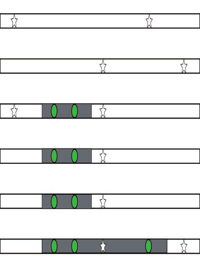
Iasi et al. . doi:10.1093/molbev/msab210                                                                                   MBE

                                                                                                                                          Downloaded from https://academic.oup.com/mbe/advance-article/doi/10.1093/molbev/msab210/6319725 by MAX PLANCK INSTITUT FUER EVOLUTIONAERE ANTHROPOLOGIE user on 02 September 2021
The first-generation offspring of an archaic and a modern            recent Neandertal ancestry less than ten generations before
human parent will have one whole chromosome each of                  hint at admixture histories with late gene flow in Europe.
either ancestry. Thus, the genomic markers in these individ-
uals are in full ancestry linkage disequilibrium (ALD); all ar-
                                                                     Limitations of the Pulse Model
chaic variants are present on one DNA molecule, and all
                                                                     The admixture pulse model assumes that gene flow occurs
modern human variants on the other one.
                                                                     over a short time period; however, it is currently unclear how
    If this individual has offspring in a largely modern human
                                                                     long a time could still be consistent with the data. This makes
population, in each generation meiotic recombination will
                                                                     admixture time estimates hard to interpret, as more complex
reshuffle the chromosomes, progressively breaking down
                                                                     admixture scenarios might be masked, and so gene flow could
the ancestral chromosome down into shorter segments of
                                                                     have happened tens of thousands of years before or after the
archaic ancestry (Falush et al. 2003; Gravel 2012; Liang and
                                                                     estimated admixture time.
Nielsen 2014), and ALD similarly decreases with each gener-
                                                                         That admixture histories are often complicated has been
ation after gene flow (Chakraborty and Weiss 1988; Stephens
                                                                     shown in the context of Denisovan introgression into modern
et al. 1994; Wall 2000).
                                                                     humans, where at least two distinct admixture events into
    This inverse relationship between admixture time and ei-
                                                                     East Asians and Papuans were proposed (Browning et al.
ther segment length or ALD is commonly used to infer the
                                                                     2018; Jacobs et al. 2019; Choin et al. 2021). Although the
timing of gene flow (Pool and Nielsen 2009; Moorjani et al.
                                                                     length distributions of admixture segments are similar be-
2011; Pugach et al. 2011, 2018; Gravel 2012; Sankararaman et
                                                                     tween populations, there are differences in the genomic dis-
al. 2012, 2016; Loh et al. 2013; Hellenthal et al. 2014; Liang and
                                                                     tribution of admixture segments, and their similarities to the
Nielsen 2014; Jacobs et al. 2019). Most commonly, it is as-
                                                                     sequenced high-coverage Denisovan (Browning et al. 2018;
sumed that gene flow occurs over a very short duration, re-
                                                                     Massilani et al. 2020). In contrast, all Neandertal admixture
ferred to as an admixture pulse, which is typically modelled as
                                                                     segments are most similar to the Vindija Neandertal (Prüfer et
a single generation of gene flow (Moorjani et al. 2011). This
                                                                     al. 2017), but Neandertal ancestry is slightly higher in East
model has the advantage that both the length distribution of
                                                                     Asians than Western Eurasians (Meyer et al. 2012; Wall et
admixture segments and the decay of ALD with distance will
                                                                     al. 2013; Kim and Lohmueller 2015; Vernot and Akey 2015;
follow an exponential distribution, whose parameter is di-
                                                                     Villanea and Schraiber 2019).
rectly informative about the time of gene flow (Pool and
                                                                         One way to refine admixture time estimates is to include
Nielsen 2009; Gravel 2012; Liang and Nielsen 2014).
                                                                     two or more distinct admixture pulses. The distribution of
    In segment-based approaches, dating starts by identifying
                                                                     admixture segment lengths will then be a mixture of the
all admixture segments, which can be done using a variety of
                                                                     segments introduced from each event. This is especially useful
methods (Seguin-Orlando et al. 2014; Sankararaman et al.
                                                                     if the events are very distinct in time, for example, if one event
2016; Vernot et al. 2016; Racimo et al. 2017; Skov et al.
                                                                     is only a few generations back, and the other pulse occurred
2018). The length distribution of inferred segments is then
                                                                     hundreds of generations ago (Fu et al. 2014, 2015). In this case,
used as a summary for dating when gene flow happened.
                                                                     the admixture segments will be either very long if they are
    Alternatively, ALD-based methods use linkage disequilib-
                                                                     recent, or much shorter if they are older.
rium (LD) patterns, without explicitly inferring the segments
                                                                         Zhou, Qiu, et al. (2017) extended this model to continuous
(Chimusa et al. 2018) (fig. 1B). Instead, admixture dates are
                                                                     mixtures, using a polynomial function as a mixture density.
estimated by fitting a decay curve of pairwise LD as a function
                                                                     However, they found that even for relatively short admixture
of genetic distance, implicitly summing over all compatible
                                                                     events, the large number of parameters led to an underesti-
segment lengths (Moorjani et al. 2011; Loh et al. 2013).
                                                                     mate of admixture duration (Zhou, Yuan, et al. 2017).
Neandertal Gene Flow Estimates
Using this approach, Sankararaman et al. (2012) dated the            Extended Pulse Model
Neandertal–human admixture pulse to between 37–86 ka.                One drawback of these approaches is that they introduce a
Later, Moorjani et al. (2016) refined this date to 41–54 ka          large number of parameters. Even a discrete mixture of two
CI95% using an updated method, a different marker ascertain-         pulses requires at least three parameters (two pulse times and
ment scheme and a refined genetic map for European pop-              the relative magnitude of the two events) (Pickrell et al. 2014),
ulations. A date of 50–60 ka was obtained from the analysis of       and the more complex models require regularization schemes
the genome of Ust’-Ishim, a 45,000-year-old modern human             for fitting (Ralph and Coop 2013; Zhou, Yuan, et al. 2017).
from western Siberia. The inferred Neandertal segments in               Here, we propose an extended admixture pulse model (fig.
Ust’-Ishim are substantially longer than those in present-day        1A) to estimate the duration of an admixture event. It only
humans, which makes their detection easier, and adds further         adds one additional parameter, reflecting the duration of
evidence that gene flow between Neandertals and modern               gene flow, while retaining much of the mathematical simplic-
humans has happened relatively recently before Ust’-Ishim            ity present in the simple pulse model. The extended pulse
lived (Fu et al. 2014). In addition, we have direct evidence         model assumes that the migration rate over time is Gamma
of gene flow from early modern humans from Oase (Fu et al.           distributed, so that the length distribution of admixture seg-
2015) and Bacho Kiro (Hajdinjak et al. 2021), dated to 40 and        ments has a closed form (fig. 1C and D) with two parameters,
45ky, respectively. In genomes from both sites, segments of          the mean admixture time and duration.
2
Extended Admixture Pulse Model . doi:10.1093/molbev/msab210 MBE
Downloaded from https://academic.oup.com/mbe/advance-article/doi/10.1093/molbev/msab210/6319725 by MAX PLANCK INSTITUT FUER EVOLUTIONAERE ANTHROPOLOGIE user on 02 September 2021
A B
C 1.0e−04 D −8
−9
7.5e−05
−10
log weighted LD
Migration Rate
5.0e−05 −11
−12
2.5e−05
−13
0.0e+00 −14
0 1000 2000 3000 0.0 0.1 0.2 0.3 0.4 0.5
Time in Generations Genetic distance (cM)
1 200 800 1500 2500
Admixture Duration
100 400 1000 2000
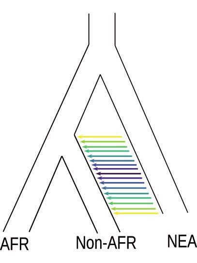
FIG. 1. (A) Neandertal introgression into non-Africans with a multitude of potential admixture durations. (B) The time and duration of admixture
results in different length distributions of introgressed chromosomal segments (gray) containing Neandertal variants (green circles) in high LD to
each other compared with the background (human variants white stars). The ALD approach estimates linkage between the introgressed variants
(green circles), whereas the haplotype approach tries to estimate the segment directly (gray area). (C) Migration rate per generation modeled using
the extended pulse model for different admixture durations (colored lines). The filled area under the curve indicates the boundaries of the discrete
realization of the duration of gene flow td. The dotted line indicates the oldest possible time of gene flow (as defined in the simulations). (D) The
expected LD decay under the extended pulse model.
Conceptually, identifying an extended pulse requires us to Here, we first define the extended admixture pulse model
establish that the length distribution of admixture segments and derive the resulting segment length and ALD distribu-
deviates from an exponential distribution. However, other sour- tions, and introduce inference schemes for either data. We
ces of bias, such as the demography of the admixed population, then evaluate under which scenarios these two models can be
the accuracy of the recombination map or details in the infer- distinguished. We show that power to distinguish these sce-
ence method parameters may also introduce similar biases. narios is higher for more recent events and longer pulses, but
Thus, we have to carefully evaluate other potential sources of that accurate inference requires high-quality data. Based on
bias on whether they might lead to confounding signals. these results, we use data from European genomes (1000
(Sankararaman et al. 2012; Fu et al. 2014; Moorjani et al. 2016). Genomes Project Consortium 2015) and find that for the
3Iasi et al. . doi:10.1093/molbev/msab210 MBE
Downloaded from https://academic.oup.com/mbe/advance-article/doi/10.1093/molbev/msab210/6319725 by MAX PLANCK INSTITUT FUER EVOLUTIONAERE ANTHROPOLOGIE user on 02 September 2021
case of Neandertal admixture, a simple pulses cannot be dis- Integrating over T yields the unconditional distribution of
tinguished from continuous admixture over an extended pe- admixture segment lengths:
riod of time, and the data are consistent with a multitude of ð1
durations, up to several tens of thousands of years. PðLi ¼ lÞ ¼ PðTi ¼ tÞPðLi ¼ ljTi ¼ tÞ dt;
ð1 0
New Approaches G
¼ t2 mðtÞetl dt
In this section, we present the mathematical description of E½K 0
the admixture models we use in this paper, and introduce
inference algorithms for estimating the admixture time and and we can think of L as an exponential mixture distribution
duration from both segment data and ALD. with mixture density proportional to tm(t) (Ralph and Coop
2013; Ni et al. 2016; Zhou, Qiu, et al. 2017).
Admixture Models and Inference
We think of admixture as a series of “foreign” chromosomes
introduced in a population (for a mechanistic model, see, e.g., Ancestry Linkage Disequilibrium
Pool and Nielsen [2009]). Throughout, we assume that alleles Alternatively, the impact of gene flow is often characterized
evolve neutrally, and that recombination is independent of using ALD, particularly when accurate identification of ar-
local ancestry. The simple pulse model assumes that all ad- chaic segments is difficult. We follow Loh et al. (2013) and
mixture happens in the same generation, (i.e., all chromo- note that the ALD from gene flow in a single event at time t
somes are introduced to the population at the same time). generations in the past is
To extend this model, we allow chromosomes to enter at Dt ¼ mð1 mÞDx Dy mA; (4)
potentially many different time points, such that the migra-
tion rate at time t in the past is given by the function m(t) where m is the fraction of immigrants and Dx ; Dy are the
(Pool and Nielsen, 2009; Ni et al. 2016). For simplicity, we differences in allele frequencies between markers in the
assume
Ð1 that the total amount of introgressed material a ¼ admixing populations. We assume that terms of the order
0 mðtÞdt is small, so that segments do not interact, but we of m2 can be ignored and that migration is low enough that
will discuss violations of this assumptions later. For archaic changes in the allele frequencies in the admixing populations
introgression, a 0:03, so this assumption is justified. can also be neglected (i.e., A ¼ Dx Dy remains a constant).
Over time, recombination splits up the introgressed ge- At a later generation s, the expected LD between two
nome into smaller pieces, whereas by the neutrality assump- markers a distance l apart is
tion the expected amount of total ancestry remains
Ds Dt expðlðs tÞÞ; (5)
approximately the same. Thus, if we measure the size of
chromosomes in recombination units, a chromosome of due to the decay of LD (Sankararaman et al. 2012). If the
size G introduced at time t gives rise to an expected number migration rate mf is a function of time, we can add up the
of tG segments. LD introduced at each time t in the past and approximate D
as
Admixture Segment Lengths ðs
We enumerate the admixture segments in a sample Ds ¼ A mf tÞexpðlðs tÞÞdt: (6)
i ¼ 1 . . . K. We denote the length of the i-th segment as Li 1
(measured in Morgan) and the time in the past when seg- As we show in the Appendix (Formal Motivation for ALD),
ment i entered the population as Ti (measured in genera- equation (6) satisfies the differential equation
tions). We assume that the Li and Ti are both realizations from
more general distributions L and T that reflect the overall dDs
¼ lDs þ Amf ðsÞ; (7)
segment length and segment age distributions, respectively. ds
To relate m(t) to T, we need to take into account that
where the lDs -term models the exponential decay of LD
older fragments had more time to split up (see, e.g., Pool and
due to recombination, and the Amf ðsÞ-term reflects the in-
Nielsen 2009). Hence
crease of LD due to admixture (eq. 4).
tGmðtÞ To connect this equation more directly to the backward-
PðTi ¼ tÞ ¼ Ð 1 : (1) in-time formulation used in the derivation of the admixture
0 tGmðtÞdt
segment distribution, we set s ¼ 0 and invert the flow of time,
The denominator of the right-hand side term in equation such that mðtÞ ¼ mf ðtÞ. We obtain
(1) is the
Ð 1 expected number of admixture segments, ð1
E½K ¼ 0 tGmðtÞdt. DðlÞ ¼ A mðtÞexpðltÞdt: (8)
Given Ti, the segment length Li is exponentially distributed 0
with rate parameter t: Thus, D can be interpreted as the tail function of an ex-
PðLi ¼ ljTi ¼ tÞ ¼ te : tl
(2) ponential mixture with mixture density m. Alternatively, the
integral in equation (8) is also the (scaled) moment-
generating function of m with argumentl.
4Extended Admixture Pulse Model . doi:10.1093/molbev/msab210 MBE
Downloaded from https://academic.oup.com/mbe/advance-article/doi/10.1093/molbev/msab210/6319725 by MAX PLANCK INSTITUT FUER EVOLUTIONAERE ANTHROPOLOGIE user on 02 September 2021
The distribution of admixture segment lengths (eq. 3) and The Extended Pulse Model
the ALD function (eq. 8) are closely related—in the Appendix For the new extended pulse model, we assume that the mi-
(Connection between Admixture Segment Length gration rate m(t) follows a rescaled Gamma distribution so
Distribution and ALD Function) we show that that the total contribution of migrant alleles is a. It is conve-
ð nient to parameterize the migration rate as C k; tkm . for t
EðKÞ 1
DðlÞ ¼ Pð xÞð x lÞdx (9) 0 and k 1.
G l Using this parameterization, the denominator of equation
(1) is tm aG and
PðlÞ / D00 ðlÞ: (10)
t
It follows that both functions uniquely determine each PðTi ¼ tÞ ¼ mðtÞ (15a)
tm
other. Consequently, they contain identical information to
estimate admixture dates. 1 k1 t k
Both for the segment and ALD models we use simplifying ¼ t k t e tm (15b)
m
assumptions that ignore the effects of genetic drift, the re- CðkÞ
k
combination between introgressed segments and the replace-
ment of older introgressed material. In the Appendix, we for t 0 and k 2, which is is the density of a C k þ 1; tkm -
discuss these approximations and show that particularly distribution with moments
the replacement of admixed material can be accommodated kþ1
by replacing m with E½T ¼ tm
k
ðt (16)
kþ1 k þ 1 td 2
me ðtÞ ¼ mðtÞexp mðsÞds ; (11) Var½T ¼ 2 t2m ¼ ð Þ:
0 k k 4
1
which can be interpreted as the probability of the event that Here, we define the admixture duration td ¼ 4tm k2 , as a
migration happened at time t, and no more migration hap- convenient measure for the duration of gene flow. If k is low,
pened later on. then td will be large and gene flow extends over many gen-
erations. In contrast, if k is large, then td 0 and we recover
the simple pulse model (fig. 1C and D).
The distribution of segment length is calculated by plug-
The Simple Pulse Model ging equation (15b) into equation (3) and integrating:
Under the simple pulse model, all fragments enter the pop- ð1
1 k1 t k tl
ulation at the same time tm, and T is a constant distribution. PðL ¼ ljk; tm Þ ¼ t k t e tm te dt
0 m
We can formalize this model by using a Dirac delta function CðkÞ
which integrates to one if the integration interval includes tm l
0 1kþ2
and zero otherwise:
Bk þ 1C
mðtÞ ¼ adtm ðTi Þ; (12a) ¼ tk B C :
m @ kA
lþ
PðTi Þ ¼ dtm ðTi Þ; (12b) tm
The distribution in equation (17) is known as a Lomax or
We obtain the exponential distribution of admixture frag-
Pareto-II distribution, which is a heavier-tailed relative of the
ments under this model (Moorjani et al. 2011):
Exponential distribution. Under the extended pulse model,
PðLi ¼ lÞ ¼ tm etm l (13a) the expected segment length will be the same as under the
simple pulse model (eq. 14a):
DðlÞ / etm l ; (13b) k 1 1
E½L ¼ ¼ (18)
where here and in the remainder of this section we omit the tm ðk þ 1Þ 1 tm
constant term from D, which is not relevant for fitting the LD but the variance is larger:
decay. The expected segment length under a simple pulse
model is given by ðk þ 1Þ 1
Var½L ¼ : (19)
1 ðk 1Þ t2m
E½L ¼ (14a)
tm We obtain the ALD-function from equation using the
and the variance by moment-generating function of m(t):
1 tm l k
Var½L ¼ : (14b) Dt ðlÞ / 1 þ : (20)
t2m k
5Iasi et al. . doi:10.1093/molbev/msab210 MBE
Downloaded from https://academic.oup.com/mbe/advance-article/doi/10.1093/molbev/msab210/6319725 by MAX PLANCK INSTITUT FUER EVOLUTIONAERE ANTHROPOLOGIE user on 02 September 2021
The Constant Migration Model generations, and sample between 100 and 100,000 unique
The simple pulse model can be thought of as the extreme segments. As the simple pulse model is an edge case of the
case of the extended pulse model when k ! 1, that is, the extended pulse model with k ! 1, standard likelihood the-
pulse gets infinitely short. In the other extreme, the extended ory does not apply, and we use empirical significance cutoffs
pulse model approaches a model of constant migration. In (Kozubowski et al. 2008).
this case, the last migration event at a particular location is The resulting log-likelihood ratios are given in figure 2.
exponentially distributed with rate m (eq. 11), which is a In general, we find that power to distinguish the model
model considered by Pool and Nielsen (2009). Setting increases with pulse duration and the amount of data, and
tm ¼ m2 ; k ¼ 2, we obtain that it is easier to distinguish the models when gene flow
had been more recent. For example, with 10,000 unique
mðtÞ ¼ mexpðmtÞ Cð1; mÞ (21a) segments we need an event lasting around 1,000 genera-
tions before we are able to confidently distinguish an ex-
PðTi ¼ tÞ Cð2; mÞ (21b)
tended from a simple pulse (fig. 2) using present-day data.
In contrast, by sampling closer to the admixture event we
2m2
PðLi ¼ lÞ ¼ (21c) are able to distinguish an extended pulse already with a
ðm þ lÞ3 duration of 40–60 generations.
m
DðlÞ / : (21d) Population Genetic Model Comparisons
mþl In the previous section, we have shown that we can distin-
Equation (21c) differs slightly from equation (6) in Pool guish long pulses from instantenous gene flow under idealized
and Nielsen (2009) because we approximate the expected conditions. As a more realistic scenario, we perform popula-
number of segments with n ¼ Kt, versus theirs n ¼ 1 þ Kt tion genetic simulations using msprime (Kelleher et al. 2016).
(however, they converge to each other for large Kt). Throughout, we simulate 3% Neandertal admixture into non-
Africans using a demographic model of archaic introgression
Estimation of Admixture Times (supplementary fig. 1B, Supplementary Material online) with
For inference, either the admixture segment lengths or ALD a mean admixture time of 1,500 generations ago and varying
can be used. Assuming the admixture segment lengths are durations. We simulate 20 chromosomes of length 150 MB,
known, equation (17) is the likelihood function and can be using either a constant recombination map or the HapMap
used for inference. For inference using ALD, we follow recombination map (International HapMap Consortium
Moorjani et al. (2011) and use the decay of ALD with genetic 2007). This results in 10; 000 introgressed segments. We
distance as a statistic. Following Moorjani et al. (2016), we add then perform inference using either the simulated segments,
an intercept A and a constant c modeling background LD: segments inferred from the data (Skov et al. 2018), or ALD
calculated using ALDER (Loh et al. 2013). We further vary
ALD Aetm l þ c (22) recombination rate settings as 1) inference and simulation
under constant recombination rate (Constant/Constant); 2)
tm k simulation using the HapMap genetic map (International
ALD A 1 þ l þ c: (23)
k HapMap Consortium 2007), and inference using no correc-
tion (HapMap/Constant); 3) simulation using HapMap, cor-
rection using a different map (HapMap/AAMap) (Hinch et al.
Results 2011); 4) and inference using the same map used for the
Here, we investigate under which scenarios we can distinguish simulations (HapMap/HapMap).
the simple and extended pulse models, and when we can Using these simulations, we perform model comparisons
infer parameters under either model. We start with an ideal- (fig. 3A). For segments, we again use the likelihood-ratio and
ized scenario of simulations under the model, and then con- find that the results for the simulated segments closely match
tinue with more realistic coalescent simulations using the simulations under the model (fig. 2), showing that our
msprime (Kelleher et al. 2016). model is a good approximation in the parameter range of
interest. In contrast, we find that for inferred segments, results
Power Analysis under the Model greatly depend on the recombination rate used: For a con-
In the easiest case, we assume that segments are known and stant recombination rate, results are similar, but for the
we simulate directly under the model (eq. 17) and evaluate HapMap-recombination map, we do not have any power
under which conditions we can tell the two models apart to distinguish these scenarios. As we fit ALD using nonlinear
using likelihood-ratio tests on the simulated segments. For least squares, no formal model-comparison framework exists.
this purpose, we compare two scenarios, one where gene flow Qualitatively, we plot the normalized residual sum-of squares
happened 1,500 generations ago, which reflects Neandertal (RSS) and find that they increase with td for both recombi-
gene flow inferred from present-day individuals. In the second nation scenarios, suggesting that the difference between the
scenario, which reflects inference from ancient modern hu- two models increase.
man data, the samples are taken 50 generations after gene Next, we evaluate parameter inference. In figure 3B, we
flow ended. We vary pulse durations from 1 to 2,500 present estimates of the mean admixture times, admixture
6Extended Admixture Pulse Model . doi:10.1093/molbev/msab210 MBE
Downloaded from https://academic.oup.com/mbe/advance-article/doi/10.1093/molbev/msab210/6319725 by MAX PLANCK INSTITUT FUER EVOLUTIONAERE ANTHROPOLOGIE user on 02 September 2021
10.0
7.5
# seg:
100
5.0
2.5
0.0
10.0
log Likelihood Ratio
7.5
# seg:
1000
5.0
2.5
0.0
10.0
7.5
10000
# seg:
5.0
2.5
0.0
10.0
100000
7.5
# seg:
5.0
2.5
0.0
1 20 40 60 80 100 400 1000 1500 2000 2500
Admixture Duration
Sampled at present Sampled 50 after end of gene flow
FIG. 2. Model comparisons on perfect data. Segments are either sampled at the present (purple) or 50 generations after the end of gene flow
(turquoise). Log-likelihood ratios bigger than 10 are rounded to 10.
duration and the fitted segment and ALD distributions, re- fragments perform poorly, which is reflected by a substantial
spectively. We find that the mean admixture times are rea- downward bias of tm and td.
sonably accurately estimated in most scenarios, the exception
being the inferred segments when using the variable Comparing Effect Sizes for Technical Covariates
(HapMap) recombination map. The admixture duration esti- As we find that ALD performs as good or better than inferred
mates are often less accurate, and in most cases has very large segments (fig. 3), we focus on ALD for the remainder of this
variation between simulations. article. Our next goal is to more carefully evaluate the relative
We detect a slight, but consistent underestimate of the importance of common assumptions made in the inference
mean admixture times, which increases with td. For the seg- of admixture times, under both the simple and extended
ments, this underestimate is likely due to the slight downward pulse models in the ALD framework on the bias and accuracy
bias caused by recombination and coalescence between of estimates of tm under either model.
admixed segments (Liang and Nielsen 2014, see also In particular, we use a Bayesian generalized linear model
Appendix Genetic Drift and Recombination). For ALD, this (GLM) framework to contrast the effect of extended gene
bias is much less severe, particularly for inference under the flow on admixture time inference with 1) the effects of a
extended pulse model. For scenarios where the recombina- simple/complex demographic history (supplementary fig. 1,
tion map is misspecified, tm is estimated to be only around Supplementary Material online); 2) recombination map var-
half of its true value (supplementary fig. 2, Supplementary iation; 3) the ALD ascertainment scheme; 4) d0, the minimum
Material online). However, we find that in some cases, the genetic distance between variants; and 5) the number of
extended pulse model provides a better estimate of tm by makers used to estimate the ALD curve (see Materials and
estimating the pulses to be extremely long. Methods for details). For each modeling parameter and gene
In figure 3C, we show examples of the estimated segment flow model, we use a simple model as the base case, and we
length and ALD distributions compared with the simulated study the impact of a more “realistic” alternative model.
data. For these log-plots, the slope of the curve corresponds In figure 4, we present the estimated effect sizes for these
to the estimate of tm, and the deviation from linearity reflects six variables and four key interaction terms. To model bias, we
the duration of gene flow. In all cases, we find that the fit a model to the standardized difference between the true
expected decay is very close to linear, matching our finding and estimated mean admixture time, and to model accuracy,
that power to differentiate these old events is limited. We find we us the absolute deviation (Materials and Methods, sup-
that particularly when using a constant recombination map, plementary table 1, supplementary fig. 3, and supplementary
all three summaries give a very close fit, and the segment table 2, Supplementary Material online). These effect sizes are
length and ALD-decay distribution closely follow their expect- estimated using simulations under all possible parameter
ations, which is consistent with the generally good parameter combinations on a scenario with admixture happening
estimates under these conditions. In the case of a variable 1,500 generations ago (supplementary figs. 4 and 5,
recombination map, we find that particularly inferred Supplementary Material online).
7Iasi et al. . doi:10.1093/molbev/msab210 MBE
Downloaded from https://academic.oup.com/mbe/advance-article/doi/10.1093/molbev/msab210/6319725 by MAX PLANCK INSTITUT FUER EVOLUTIONAERE ANTHROPOLOGIE user on 02 September 2021
10.0
A B 2500
Admixture Duration
2000
7.5
Extended Pulse
True Segments
Estimated
1500
5.0
1000
2.5
500
log Likelihood
0
Ratio
0.0
10.0
2500
Extended Pulse
7.5 2000
Inferred Segments
5.0 1500
Admixture Time
Estimated Mean
1000
2.5
2500
0.0
Simple Pulse
2000
0.00
1500
RSS Difference
−0.25 1000
Normalized
tm = 1500 tm = 1500 tm = 1500 tm = 1500
ALD
−0.50 td = 1 td = 1000 td = 1500 td = 2000
Inferred Segments
Inferred Segments
Inferred Segments
Inferred Segments
True Segments
True Segments
True Segments
True Segments
−0.75
ALD
ALD
ALD
ALD
td = 1 td = 1000 td = 1500 td = 2000
Recombination Constant/Constant HapMap/HapMap
C True Segments True Segments Inferred Segments Inferred Segments ALD ALD
td = 1 td = 2000 td = 1 td = 2000 td = 1 td = 2000
−2.75
Constant/Constant
−3.00
3.0
−3.25
2.5 −3.50
log weighted LD
−3.75
log density
2.0 −4.00
−2.75
HapMap/HapMap
−3.00
3.0
−3.25
2.5 −3.50
−3.75
2.0 −4.00
0.001
0.002
0.003
0.001
0.002
0.003
0.001
0.002
0.003
0.001
0.002
0.003
0.001
0.002
0.003
0.001
0.002
0.003
Genetic distance (M) Genetic distance (M)
Fit True fitted SP fitted EP
FIG. 3. Model choice, model fit, and parameter estimates. (A) Log-likelihood ratios and RSS difference between the simple and extended pulse
models for segment data and ALD, respectively. Simulation and inference were done using constant (purple) and an empirical (teal) recombi-
nation map. (B) Estimates of tm and td. Solid black line indicates simulation values, the red dotted line adds a migration corrected (tm ð1 aÞ). (C)
Model fit for a single simulation in each scenario. Estimated segment density or weighted LD (gray) is compared with the expected (turquoise) and
fitted single pulse (yellow) and extended pulse (purple).
8Extended Admixture Pulse Model . doi:10.1093/molbev/msab210 MBE
Downloaded from https://academic.oup.com/mbe/advance-article/doi/10.1093/molbev/msab210/6319725 by MAX PLANCK INSTITUT FUER EVOLUTIONAERE ANTHROPOLOGIE user on 02 September 2021
Model Simple Pulse Extended Pulse
0.5
Standardized dif.
est./sim. time
0.0
bias
−0.5
−1.0
Standard Model
Extended Pulse
Varying
Recombination
Complex
Demography
d0 = 0.02
HES
n SNP = 5%
Interaction
n SNP = 5%/HES
Interaction
Complex D./Varying R.
Interaction
d0 = 0.02/HES
Interaction
d0 = 0.02/Varying R.
FIG. 4. GLM effect sizes for the bias between simulated and estimated mean admixture time and 95% CI for the parameters between the simple and
extended pulse models: gene flow (simple/extended), recombination rate (constant/varying), demography (simple/complex), minimal genetic
distance (0.02/0.05 cM), SNPs used for ALD calculation (100%/5%), and ascertainment scheme (LES/HES). Estimates are calculated across all
possible combinations of parameters. Dotted horizontal line indicates unbiased admixture estimates.
As a baseline, for comparison, we define a standard model becomes more apparent if we log-transform the y-axis (fig.
using a simple demography (supplementary fig. 1A, 5B), where we see that ongoing gene flow results in a heavier
Supplementary Material online) and a constant recombina- tail in the ALD distributions. However, these LD values are
tion rate. This baseline model results in unbiased estimates of very close to zero, and are thus only very noisily estimated.
tm under the single pulse model with low deviation of 0.08 For short gene flows (less than 1,000 generations), our
(0.02–0.14 CI95%), and a slight upward bias 0.21 (0.15–0.28) for estimates for tm are very similar and identical to the simple
the extended pulse model. pulse, at around 1,682 (1,526–1,839 CI95%) generations.
The effect of simulating an extended-pulse gene flow only Extremely high values of td result in slightly higher values of
results in a slight bias of 0.17; (0.21 to 0.13) for the tm with overlapping compatibility intervals; but all predict
simple pulse and no bias for inference under the extended that Neandertals would have survived until 30 ka, for which
pulse model (0.11; 0.15 to 0.07). In contrast, uncertainty the archeological evidence is extremely sparse (Hublin 2017).
in the genetic map causes by far the largest downward bias From the RSS, the models perform equally well, with longer
(simple pulse: 1.22, 1.29 to 1.16; extended pulse: 0.74, extended pulses of gene flow achieving marginally better fits
0.80 to 0.67) with high deviation in the estimates (sup- (supplementary table 4, Supplementary Material online).
plementary fig. 3, Supplementary Material online). The more Therefore, we find that all scenarios are compatible with
complex demography results in an underestimate of tm, pre- the observed data, and that there is little power to differen-
sumably because of increased genetic drift, for both the sim- tiate these cases from genetics alone.
ple pulse (0.27, 0.33 to 0.22) and extended pulse models
(0.43, 0.49 to 0.38). The remaining parameters largely Sampling Closer to the Admixture Event
only have very minor effects, the biggest of which is changing Since Neandertal gene flow happened long in the past, much
the minimum cutoff from 0.05 to 0.02 cM. of the signal has been lost, and we have shown that in this
scenario, power to distinguish different scenarios is low.
Application to Neandertal Data However, we have also shown in figure 2 that inference is
Our next aim is to apply our model on the case of Neandertal easier for more recent gene flow, a case that is relevant for
gene flow into Eurasians. We estimate the Neandertal admix- many study systems. We investigate this in a series of simu-
ture pulse from the 1000 Genomes data (1000 Genomes lations where the time between sampling and gene flow is
Project Consortium 2015) and three high-coverage smaller (fig. 6). We use the simple demographic scenario with
Neandertal genomes (Prüfer et al. 2013, 2017; Mafessoni et a constant-sized populations (supplementary fig. 1,
al. 2020) by fiting pulses with durations ranging from 1 gen- Supplementary Material online), and use ALD for inference
eration up to 2,500 generations to the ALD-decay curve (fig. 5, using the optimized settings for the Neandertal case (ascer-
supplementary table 3, Supplementary Material online). tainment scheme ¼ LES and d0 ¼ 0.05 cM).
Plotting these best-fit ALD curves shows the extremely slight In figure 6A and B, we show the accuracy of estimating td
difference predicted under these drastically different gene and tm for increasingly longer pulses, sampled 50 generations
flow scenarios (fig. 5A). The difference between scenarios after gene flow ended. The corresponding comparison of
9Iasi et al. . doi:10.1093/molbev/msab210 MBE
Downloaded from https://academic.oup.com/mbe/advance-article/doi/10.1093/molbev/msab210/6319725 by MAX PLANCK INSTITUT FUER EVOLUTIONAERE ANTHROPOLOGIE user on 02 September 2021
A B
−2
0.0075
−3
log weighted LD
weighted LD
0.0050
−4
0.0025
−5
0.0000
0.001 0.002 0.003 0.004 0.005 0.001 0.002 0.003 0.004 0.005
Genetic distance (M) Genetic distance (M)
SP EP td = 100 EP td = 400 EP td = 1000 EP td = 2000
Fit
EP td = 1 EP td = 200 EP td = 800 EP td = 1500 EP td = 2500
FIG. 5. Neandertal gene flow in modern humans. We fit models with fixed td from 1 to 2,500 generations of gene flow to the ALD-curve calculated
from CEU individuals on (A) natural and (B) log-scale.
model fit is depicted in supplementary figure 6, show that both the instantaneous pulse and constant migra-
Supplementary Material online. For these cases, we find tion models are special cases of our model, where the dura-
that inference of tm under the simple pulse model works tion is extremely short or long, respectively. We also
well for the shortest pulses but becomes increasingly down- demonstrate that the segment length distribution and
ward biased as td increases. Estimates of tm are less biased for ALD-decay can be directly transformed into each other; in
inference under the extended pulse model, where we get particular, the segment-length distribution is proportional to
accurate estimates particularly if recombination is constant. the second derivative of the ALD-decay curve. This makes our
In the scenarios with a variable recombination rate, we find theory and models generally applicable beyond gene flow
that for short, recent pulses, all corrections give good results, between Neandertals and humans. In fact, we find that we
but for longer pulses, particularly assuming a constant recom- have little resolution for the parameter settings relevant for
bination rate leads to a stronger bias. We also find that we are archaic gene flow, as the data resulting from simple and ex-
able to accurately infer the admixture duration, particularly if tended pulses long in the past are extremely similar. In con-
the recombination rate is constant. trast, we have much more power to estimate the duration of
In 6C and D, we keep the pulse duration constant at td ¼ gene flow from events in the recent past, a scenario relevant
800 but move it successively further into the past. For the first for many hybridizing species. One limitation of our approach
two cases of tm ¼ 450 and tm ¼ 500 where the pulse is recent, is that we assume that the overall amount of introduced
we again obtain good parameter estimates, but performance material is low, and that we ignore the effects of genetic drift
deteriorates for tm 600, which also results in low power to and selection.
distinguish the simple and extended pulse model (supple- Previous approaches to date Neandertal–human gene
mentary fig. 6, lower panel, Supplementary Material online). flow have focused almost entirely on the mean time of
gene flow using a simple pulse model, for which reasonably
Discussion tight credible intervals can be estimated (Sankararaman et al.
In this article, we introduce a new population genetic model 2012; Moorjani et al. 2016). Under this model, the credible
for dating extended pulses of gene flow. Our model has just intervals of this time are bounds of when gene flow between
two parameters, that can be interpreted as the mean time Neandertals and early modern humans could have happened.
and duration of gene flow; and has simple closed form sol- Our estimate of the tm for Neandertal gene flow of 1,682
utions for the segment length and ALD distributions. We generations corresponds to a mean time estimate of 49 ky
10Extended Admixture Pulse Model . doi:10.1093/molbev/msab210 MBE
Downloaded from https://academic.oup.com/mbe/advance-article/doi/10.1093/molbev/msab210/6319725 by MAX PLANCK INSTITUT FUER EVOLUTIONAERE ANTHROPOLOGIE user on 02 September 2021
A Simple Pulse Extended Pulse B Extended Pulse
tm = 50.5
tm = 50.5
td = 1
td = 1
tm = 150
tm = 150
td = 200
td = 200
tm = 250
tm = 250
td = 400
td = 400
tm = 450
tm = 450
td = 800
td = 800
td = 1000
td = 1000
tm = 550
tm = 550
td = 1500
td = 1500
tm = 800
tm = 800
0 500 1000 1500 0 500 1000 1500 0 500 1000 1500 2000 2500 3000 3500 4000
Estimated Admixture Mean Time Estimated Admixture Duration
C Simple Pulse Extended Pulse D Extended Pulse
tm = 450
tm = 450
td = 800
td = 800
tm = 500
tm = 500
td = 800
td = 800
tm = 600
tm = 600
td = 800
td = 800
tm = 800
tm = 800
td = 800
td = 800
tm = 1400 tm = 1200
tm = 1400 tm = 1200
td = 800
td = 800
td = 800
td = 800
0 500 1000 1500 0 500 1000 1500 0 500 1000 1500 2000 2500 3000 3500 4000
Estimated Admixture Mean Time Estimated Admixture Duration
Simulations Constant/Constant HapMap/HapMap HapMap/AAMap HapMap/Constant
FIG. 6. Parameter estimation using ALD from recent admixture pulses. We show estimates of tm (panels A, C) and td (Panels B and D) for a series of
simulations with increasing td and tm such that we sample 50 generations after gene flow (top) and a series of simulations with an increasingly older
extended pulse (bottom). All times are given in generations.
(assuming a generation time of 29 years; Moorjani et al. 2016), Neandertals survive until around 30 ka, whereas archeological
with bounds of 44–54 ky. This is in almost perfect agreement evidence for Neandertals surviving beyond 40 ky is increas-
with the previous result of Moorjani et al. (2016) (41–54 ky), ingly sparse (Hublin 2017), so that these models of extremely
which is based on largely the same method. However, here we long gene flow might be rejected on these grounds.
show that models of extended gene flow with td up to a Our finding that the observed data are compatible with
thousand generations provide very similar fits to the data; models involving hundreds of generations of gene flow means
and that marginally better fits are achieved with very long that while likely substantial amounts of gene flow happened
gene flows. However, these models all would have around these mean times, gene flow might have also
11Iasi et al. . doi:10.1093/molbev/msab210 MBE
Downloaded from https://academic.oup.com/mbe/advance-article/doi/10.1093/molbev/msab210/6319725 by MAX PLANCK INSTITUT FUER EVOLUTIONAERE ANTHROPOLOGIE user on 02 September 2021
happened tens of thousands of years before or after. This is of variance in ALD or segment lengths, which might be con-
great practical importance, as it makes linking genetic admix- founded with a longer admixture pulse (Sankararaman et al.
ture date estimates with biogeographical events much more 2012). Therefore, population-specific fine-scale recombina-
difficult (Sankararaman et al. 2012; Lazaridis et al. 2016; Douka tion maps are needed for accurate admixture time estimates,
et al. 2019; Jacobs et al. 2019; Vyas and Mulligan 2019). at least for admixture that happened more than a thousand
The discovery of early modern human genomes dated to generations ago. Estimates of more recent admixture appear
40,000–45,000 ya with very recent Neandertal ancestors less to be more robust, perhaps because coarser-scale recombi-
than ten generations ago (Fu et al. 2014; Hajdinjak et al. 2021) nation maps are better estimated, differ less between popu-
illustrates that gene flow likely happened over at least several lations (Hinch et al. 2011) and the error relative to fragment
thousand years. In general, inference based on ancient length is substantially lower.
genomes (Fu et al. 2014, 2015; Moorjani et al. 2016; To further refine admixture time estimates, time series
Hajdinjak et al. 2021) promises to resolve some of these dating data from more admixed early modern human and
issues, as inference is substantially easier when admixture is Neandertal genomes are needed. In particular, measures
more recent, as the time difference between gene flow and based on population differentiation (Wall et al. 2013;
sampling time is much lower (figs. 2 and 6). However, using Browning et al. 2018; Villanea and Schraiber 2019) hold
these genomes for dating leads to further hurdles, particularly much promise to understand the different events that con-
pertaining to the spatial distribution of admixture events; tributed to archaic ancestry in modern humans. Although
whereas we can assume that the spatial structure present Neandertal ancestry in present-day people has been largely
in initial upper paleolithic modern humans is largely homog- homogenized due to the substantial gene flow between pop-
enized in present-day people, the introgression signals ob- ulations, samples from both the Neandertal and early modern
served in Bacho-Kiro and Oase could be partially private to human populations immediately involved with the gene flow
these populations, and thus these populations may have a could refine when and where this gene flow happened.
different admixture time distribution than present-day
people. Materials and Methods
The uncertainty over the duration of Neandertal gene flow
also has some implications for selection on introgressed Power Analysis under the Model
Neandertal haplotypes. Neandertal alleles have been sug- To test the power to distinguish the simple from an extended
gested to be deleterious in modern human populations due pulse we simulated 100, 1,000, 10,000, and 100,000 unique
to an increased mutation load (Harris and Nielsen 2016; Juric times Ti from a Gamma distribution, with shape parameter
et al. 2016). Some details of these models may be affected if k þ 1 and scale k=tm , setting tm to 1,500 generations. Segment
migration occurred over a longer time. For example, Harris lengths Li are obtained by sampling for each Ti from an ex-
and Nielsen (2016) suggested that an initial pulse of gene flow ponential distribution with rate parameter Ti for present day
ðcloserÞ
of up to 10% Neandertal ancestry might be necessary to ex- samples and Ti ¼ Ti tm td =2 50 for sampling 50
plain current amounts of Neandertal ancestry, with very high generations after the end of gene flow. We obtain maximum-
variance in the first few generations after gene flow. More likelihood estimates for the simple (Eq. 13a) and extended
gradual gene flow could mean that such high admixture pulse (Eq. 17) using the optim function implemented in R (R
proportions were never reached, but rather a continuous Core Team 2019).
migration–selection balance process persisted for the contact
period, where deleterious Neandertal alleles continually en- Coalescent Simulations
tered the modern human populations, but were selected We further test our approach on coalescence simulations
against immediately. However, in terms of the overall fre- using msprime (Kelleher et al. 2016). We focus on scenarios
quencies, there is likely little difference. For example, Juric et mimicking Neandertal admixture and choose sample sizes to
al. (2016) showed using a two-locus model that the frequen- reflect those available from the 1000 Genomes data (1000
cies of Neandertal haplotypes alone cannot be used to dis- Genomes Project Consortium 2015). For ALD simulations,
tinguish different admixture histories. we simulate 176 diploid African individuals and 170 diploid
In addition, we find that modeling and method assump- non-Africans, corresponding to the number of Yoruba (YRI)
tions have an impact on admixture time estimates that are of and Central Europeans from Utah (CEU). For inference based
a similar or larger magnitude than the effect of assuming a on segments, we simulated 50 diploid non-Africans. Since
one-generation pulse. In particular, recombination rate vari- three high-coverage Neandertal genomes are available
ation poses a practical limitation to the accuracy of admixture (Prüfer et al. 2013, 2017; Mafessoni et al. 2020), we simulate
date estimates for old gene flow, and has to be very carefully three diploid Neandertal genomes.
considered when making inferences about admixture times. The demographic parameters are based on previous stud-
A possible reason is that both an extended pulse as well as a ies dating Neandertal admixture (Sankararaman et al. 2012;
nonhomogeneous recombination map lead to an admixture Fu et al. 2014; Moorjani et al. 2016; Skov et al. 2018). In the
segment distribution that deviates from the expected expo- “simple” demographic model (supplementary fig. 1A,
nential distribution. Throughout, we measure segment Supplementary Material online), the effective population
lengths and LD-decay distance in recombination units. size is assumed constant at Ne ¼ 10; 000 for all populations,
Misspecification of the recombination rate will increase the the split time between modern humans and Neandertals is
12Extended Admixture Pulse Model . doi:10.1093/molbev/msab210 MBE
Downloaded from https://academic.oup.com/mbe/advance-article/doi/10.1093/molbev/msab210/6319725 by MAX PLANCK INSTITUT FUER EVOLUTIONAERE ANTHROPOLOGIE user on 02 September 2021
10,000 generations, and the split between Africans and non- Estimating Admixture Time from Simulated Segment
Africans is 2,550 generations. The migration rate from Data
Neandertals into non-Africans was set to zero before the split For estimating admixture time and duration from intro-
from Africans, to ensure that there is no Neandertal ancestry gressed segments, we either used the simulated segment
in Africans. For a more complex scenario of human popula- lengths directly or alternatively added an inference step using
tion history, we followed Skov et al. (2018) and used a similar the HMM from Skov et al. (2018). We only considered in-
demographic model, but only simulated the Europeans. We ferred segments with an average posterior probability of 0.9 or
changed the Ne for the ancestral humans, out-of-Africa bot- higher. Furthermore, we use an upper and lower cutoff for
tleneck and ancestral Eurasians to 7,000, 250, and 5,000, re- inferred segment length of 0.05 and 1.2 cM. We fit the simple
spectively. The effective population size for Neandertals was (eq. 13a) and extended pulse (eq. 17) using the optim func-
set to 5,000 and the split time of non-Africans is kept the tion implemented using R 4.0.3 (method¼“L-BFGS-B”) with
same as in the ALD simulations (2,550 generations ago) (sup- lower and upper constrains being 1 and 5,000 for tm and 2
plementary fig. 1B, Supplementary Material online). and 1010 for k, respectively.
For each individual, we simulate 20 chromosomes with a
length of 150 Mb each. The mutation rates are set to 2 1 Estimating Admixture Time from ALD Data
08 and 1:2 108 per base per generation for the “simple” Ascertainment Scheme
and “complex” models, respectively. The recombination rates Since ALD for ancient admixture events can be quite similar
are set to 1 108 per base pair per generation for the sim- to the genomic background, SNPs need to be ascertained to
ple demography and 1:2 108 per base pair per generation enrich for Neandertal informative sites in the test population.
for the complex demographic model, unless specified This removes noise and amplifies the ALD signal
otherwise. (Sankararaman et al. 2012). We evaluate the impact of the
Since inferring archaic segments is slow, we use 25 repli- ascertainment scheme by contrasting two distinct schemes
cates for scenarios where we compare segment-based and (Sankararaman et al. 2012; Fu et al. 2014). The lower-
ALD-based inference and use 100 replicates when we only enrichment ascertainment scheme (LES) only considers sites
perform ALD-based inference. that are fixed for the ancestral state in Africans and polymor-
phic or fixed derived in Neandertals. The higher-enrichment
Simulating Admixture ascertainment scheme (HES) is more restrictive in that it
We specify simulations under the extended pulse model using further excludes all sites that are not polymorphic in non-
the mean admixture time tm and the duration td. We recover Africans.
the simple pulse model by setting td ¼ 1, up to errors due to
discrete generations. To obtain the migration rates in each
generation, we use a discretized version of the migration den- ALD Calculation
sity (eq. 15b), which we then scale to the approximate The pairwise weighted LD between the ascertained SNPs a
amount of Neandertal ancestry in non-Africans (a ¼ 0:03). certain genetic distance d apart is calculated using ALDER
(Loh et al. 2013). A minimal genetic distance d0 between
Recombination Maps SNPs is set to either 0.02 or 0.05 cM. This minimal distance
cutoff removes extremely short-range LD, which might also
Uncertainties in the recombination map were previously
be due to inheritance of segments from the ancestral popu-
shown to influence admixture time estimates
lation (incomplete lineage sorting ILS) and not gene flow.
(Sankararaman et al. 2012, 2016; Fu et al. 2014). To investigate
the effect of more realistic recombination rate variation, we
perform simulations using empirical recombination maps. Parameter Estimates
For the GLM, we use the African-American map (Hinch et We estimate parameters by fitting the ALD-curve to equa-
al. 2011) for simulations and for the remaining simulations we tions (22) and (23) using a nonlinear least square approach
use the HapMap phase 3 map (International HapMap implemented in the nls function in R 4.0.3 (algo-
Consortium 2007). For simplicity, we use the same recombi- rithm¼“port”) with lower and upper constrains being 1
nation map (150 Mb of chromosome 1, excluding the first and 5,000 for tm and 1=1010 and 1/2 for 1=k, respectively.
and last 10 Mb) for all simulated chromosomes. When sim- To achieve better conversion, we prefit the functions using
ulating under an empirical map, with the analysis assuming a the estimates of the DEoptim optimization (Ardia et al. 2016)
constant rate (i.e., no correction), we use the mean recombi- as starting parameters for the nls function. To improve esti-
nation rate from the respective map to calculate the genetic mates for td, we run the fitting using ten iterations to avoid
distance from the physical distance for each SNP. The mean local optima. We select the estimate with the lowest RSS.
recombination rate is calculated from the 150-Mb map
cM cM Modeling Parameter Effect Sizes
(1:017 Mb AAMap, 0:992 Mb HapMap). For inference, each
segment is either assigned a length based on its physical To estimate the effect size of the different parameters (eq. 24)
length (“constant”), the African-American map or HapMap we use a Bayesian GLM, where E is the response, and A; M;
recombination map, depending on the inference scenario. D; R; S; and G are binary predictors.
13You can also read


