Post-Wildfire Debris Flow and Large Woody Debris Transport Modeling from the North Complex Fire to Lake Oroville
←
→
Page content transcription
If your browser does not render page correctly, please read the page content below

water
Article
Post-Wildfire Debris Flow and Large Woody Debris Transport
Modeling from the North Complex Fire to Lake Oroville
Thad Wasklewicz *, Aaron Chen                    and Richard H. Guthrie

                                         Stantec, 3325 South Timberline Road Suite 150, Fort Collins, CO 80521, USA
                                         * Correspondence: thad.wasklewicz@stantec.com

                                         Abstract: The increase in wildfires across much of Western United States has a significant impact
                                         on the water quantity, water quality, and sediment and large woody debris transport (LWD) within
                                         the watershed of reservoirs. There is a need to understand the volume and fate of LWD transported
                                         by post-wildfire debris flows to the Lake Oroville Reservoir, north of Sacramento, California. Here,
                                         we combine debris flow modeling, hydrologic and hydraulic modeling, and large woody debris
                                         transport modeling to assess how much LWD is transported from medium and small watersheds to
                                         Lake Oroville. Debris flow modeling, triggered by a 50-year rainfall intensity, from 13 watersheds,
                                         transported 1073 pieces (1579.7 m3 ) of LWD to the mainstem river. Large woody debris transport
                                         modeling was performed for 1-, 2-, 5-, 25-, 50-, 100-, and 500-year flows. The transport ratio increased
                                         with discharge as expected. LWD is transported to the reservoir during a 2-year event with a transport
                                         ratio of 25% with no removal of LWD and 9% with removal of LWD greater than the cross-section
                                         width. The 500-year event produced transport ratios of 58% and 46% in our two sub scenarios.

                                         Keywords: large woody debris; debris flows; woody debris transport modeling; reservoir

                                         1. Introduction
                                              Large woody debris (LWD) in post-wildfire settings can have both deleterious, as
Citation: Wasklewicz, T.; Chen, A.;
                                         well as positive, impacts on watersheds. Debris dams formed when LWD jams can reduce
Guthrie, R.H. Post-Wildfire Debris
Flow and Large Woody Debris
                                         downstream impacts of debris floods and debris flows by trapping sediment and wood
Transport Modeling from the North
                                         in headwater streams [1,2]. Conversely, LWD transport represents a threat to infrastruc-
Complex Fire to Lake Oroville. Water     ture, recreation, and water quality in reservoirs. California has seen a recent increase in
2023, 15, 762. https://doi.org/          wildfire frequency and magnitude, which has led to large tracts of burned areas within
10.3390/w15040762                        the watersheds of many reservoirs. A need exists to understand the transport and fate
                                         of LWD standing and on the ground from the burned sub watersheds to reservoirs to
Academic Editors: Olga Petrucci
                                         better understand the sources, amount, and timing, and how to manage it once it arrives at
and Cristiana Di Cristo
                                         the reservoirs.
Received: 18 November 2022                    The transport of LWD from unburned watersheds to reservoirs in Japan has been
Revised: 20 December 2022                found to be high in small drainage basins (6–20 km2 ), highest in medium drainage basins
Accepted: 8 February 2023                (20–100 km2 ), and generally least high from the largest watersheds (>100 km2 ) [3]. The
Published: 15 February 2023              added dimension of wildfire impacts may increase the frequency and volume of LWD
                                         transport. Large floods are associated with the largest volume of LWD arriving within
                                         reservoirs, but there are often wide ranges of LWD volumes identified with large flow
                                         events [4]. Wood arriving at the reservoir is also dependent on the timing and contributions
Copyright: © 2023 by the authors.
                                         from tributary streams to the mainstem stream, forest stand characteristics, and LWD
Licensee MDPI, Basel, Switzerland.
                                         availability based on antecedent floods [4].
This article is an open access article
                                              Fire intensity has also been shown to be an important mechanism in the availability
distributed under the terms and
                                         of LWD, as very intense fires can sometimes burn away wood that is standing and on the
conditions of the Creative Commons
Attribution (CC BY) license (https://
                                         ground. In these scenarios, LWD transport might be reduced because of the lack of available
creativecommons.org/licenses/by/
                                         LWD [5]. Wildfires may also decrease the size of LWD available for transport [6]. LWD has
4.0/).                                   been found to jam and concentrate along channel margins and secondary channels during

Water 2023, 15, 762. https://doi.org/10.3390/w15040762                                                        https://www.mdpi.com/journal/water
Water 2023, 15, 762                                                                                            2 of 23

                      fluvial transport in rivers with floodplains [5]. These same areas have also been identified
                      to retain greater volumes of sediment storage following a wildfire [7].
                            Much of the literature reports greater amounts of LWD transport from recently burned
                      watersheds [1]. Burned standing trees often topple from windy conditions or the decom-
                      position of woody material providing a significant source of LWD after a wildfire [2,8,9].
                      The transport of LWD can be enhanced because of the increased magnitude and frequency
                      of debris floods and “clear water” flooding [10] and, in steep terrain, the increased po-
                      tential for debris flow occurrence [11]. Each of these mechanisms have the potential to
                      transport LWD on the ground as well as standing LWD, but this will vary depending on
                      fire conditions and the time since the fire.
                            While some studies have indicated that LWD inhibits debris flow runout [12], sub-
                      stantial amounts of LWD are transported via debris flows [13,14]. Studies of streams in
                      Northern California have shown that as much as 7% of the LWD input to streams occurs
                      from mass wasting under background conditions (without wildfires) and found that most
                      of the LWD recruitment takes place within 10 to 35 m of the channel [15].
                            Debris flows are a process that enhances the hillslope-channel connectivity following
                      wildfires, thereby increasing the sediment and LWD arriving at the mainstem stream [16,17].
                      LWD is transported along the debris flow pathways to debris flow fans or deposited within
                      the floodplain of a higher order stream than the stream order the debris flow originated
                      from. LWD deposition is often localized to the lateral portions of the debris flow fans, as
                      well as the fan toe [13,14]. Once the LWD has been transported from the tributary (feeder
                      stream) to the fan along the higher order river, it is subjected to entrainment, transport, and
                      deposition during flooding along the mainstem river [5]. Two-dimensional Eulerian and
                      Lagrangian hydrodynamic models have often been applied to model LWD [18].
                            There have been numerous attempts to model LWD transport. Initial numerical
                      modeling of LWD evolved from and in conjunction with flume experiments [19]. The
                      simulation of LWD transport using these types of models have been on force balances
                      between the wood and water [20], simulating bed deformation by LWD [21], and examining
                      multiple local forces on cylindrical wood [22]. Another approach to modeling LWD has
                      been to simulate the spatial and temporal transport across a defined space at the resolution
                      of a single tree to understand the fate of the LWD [23]. LWD transport modeling after
                      wildfires has not been a significant topic of investigation.
                            Both empirical and numerical models have been applied to understanding debris flow
                      hazards [24]. Debris flow models are typically calibrated to past real events in a trial-and-
                      error procedure [25]. A trial-and-error procedure is dictated for many reasons, such as
                      the limited understanding of how to parameterize the debris flow initiation, debris flow
                      physics, debris flow volumes, among other item because there is not a centralized historical
                      database of debris flows comparable to stream discharge in many parts of the world.
                      There are also numerous algorithms and approaches to modeling debris flows [26–28] and
                      generally no acceptable methodology for producing a potential outcome.
                            There has been an increasing volume of research modeling post-wildfire debris
                      flows [27,29–31]. Modeling in the post-wildfire arena, much like the modeling of de-
                      bris flows in general, has been focused on initiation, pathways, runout, inundation, velocity,
                      and volumes, as these items become critical to our assessing the potential risks associated
                      with these events. While debris flows play a significant role in the transport of LWD there
                      have been limited attempts to model LWD transport via debris flow models. This is an area
                      in need of further research and is critical to understanding the cascading events that take
                      place within steep channels.
                            Here, a combination of debris flow, hydrodynamic, and large woody debris transport
                      modeling are combined to assess the potential spatial and temporal movement of LWD
                      from local medium and small watersheds to Lake Oroville (Figure 1). The models are
                      calibrated to local conditions within the study area using a variety of sources of information
                      for each model. The work also considers a scenario whereby LWD is removed by jamming
                      processes throughout the extent of its transport history in Middle Fork of the Feather River
Water 2023, 15, x FOR PEER REVIEW                                                                                             3 of 24

Water 2023, 15, 762             calibrated to local conditions within the study area using a variety of sources of infor-
                                                                                                                      3 of 23
                                mation for each model. The work also considers a scenario whereby LWD is removed by
                                jamming processes throughout the extent of its transport history in Middle Fork of the
                                Feather River (MF Feather River). The scenario is designed to consider the worst-case sce-
                                (MF Feather River). The scenario is designed to consider the worst-case scenario (all LWD
                                nario (all LWD can be transported to Lake Oroville) as well as trying to mimic natural
                                can be transported to Lake Oroville) as well as trying to mimic natural processes along the
                                processes along the transport pathway (LWD being removed in jams).
                                transport pathway (LWD being removed in jams).

                                Figure 1.
                                Figure    Map of
                                       1. Map of the
                                                 the study
                                                     study location
                                                           location showing
                                                                    showing the
                                                                            the 13
                                                                                13 watersheds
                                                                                   watersheds in
                                                                                              in relation
                                                                                                 relation to
                                                                                                          to Lake
                                                                                                             Lake Oroville.
                                                                                                                  Oroville.
                                2. Study Area and Methods
                                2.1. Study Area
                                     Sites analyzed in this study are located along the canyon section of the MF Feather
                                River in Northern California. Accelerated uplift that occurred between 3.5–5 Ma caused
                                the base-level lowering in the MF Feather River [32,33]. The study area has three distinct
                                geomorphological domains as the landscape responds to the waves of aggression [34] that
                                result from this base-level lowering. Landscape evolution along the MF Feather River
                                plays a dominant role in debris flow formation and propagation throughout the drainage
                                system impacted by the North Complex Fire (2020). The lower portion of the watersheds
                                are topographically steeper and debris flows are more likely to reach the MF Feather River.
River in Northern California. Accelerated uplift that occurred between 3.5–5 Ma caused
                      the base-level lowering in the MF Feather River [32,33]. The study area has three distinct
                      geomorphological domains as the landscape responds to the waves of aggression [34] that
                      result from this base-level lowering. Landscape evolution along the MF Feather River
Water 2023, 15, 762
                      plays a dominant role in debris flow formation and propagation throughout the drainage     4 of 23
                      system impacted by the North Complex Fire (2020). The lower portion of the watersheds
                      are topographically steeper and debris flows are more likely to reach the MF Feather
                      River. Similarly, smaller sub-watersheds within these units are themselves generally
                       Similarly,
                      steeper andsmaller
                                   debris sub-watersheds
                                          flows can travel within
                                                           beyondthese
                                                                   theirunits are themselves
                                                                          immediate  watershed generally
                                                                                                  directlysteeper  and
                                                                                                           to the MF
                       debris flows can travel beyond  their immediate   watershed  directly to the MF  Feather
                      Feather River. The transitional domain occupies many of the tributary basins, thereby cre- River.
                       The transitional domain occupies many of the tributary basins, thereby creating a steeper
                      ating a steeper lower portion and a less steep upper portion of the watersheds as the en-
                       lower portion and a less steep upper portion of the watersheds as the energy line moves
                      ergy line moves upstream in response to base-level lowering [35]. This has resulted in a
                       upstream in response to base-level lowering [35]. This has resulted in a landscape that
                      landscape that currently exhibits a prominent convexity in the tributary watersheds. The
                       currently exhibits a prominent convexity in the tributary watersheds. The upper watersheds
                      upper watersheds have a lower-relief landscape with erosion rates an order of magnitude
                       have a lower-relief landscape with erosion rates an order of magnitude lower [36]. While
                      lower [36]. While  slopes > 30° are found in the upper portion of the drainage, landslide
                       slopes > 30◦ are found in the upper portion of the drainage, landslide propagation across
                      propagation across lower slopes keep debris flows within the domain (Figure 2).
                       lower slopes keep debris flows within the domain (Figure 2).

                      Figure
                       Figure2.2.AA6 6mmcontour
                                         contourmap
                                                 mapofofwatershed
                                                         watershedM7M7showing
                                                                       showingthe
                                                                                thesteeper
                                                                                     steepertopography
                                                                                             topographyininthe
                                                                                                            thelower
                                                                                                                 lowerportion
                                                                                                                       portion
                      ofofthe
                           thewatershed
                               watershedwhen
                                          whencompared
                                                comparedwith
                                                           withthe
                                                                theupper
                                                                    upperportion
                                                                          portionofofthe
                                                                                      thewatershed.
                                                                                         watershed.

                       2.2. Watershed Selection
                            USGS watershed-scale probability of debris flow occurrence was used to randomly
                       select the 8 medium and 5 small watersheds for this project [37]. Medium and small
                       watersheds are based on a local measure of watershed area and would be considered small
                       when compared with previous research from Japan [3]. The site selection was based on the
                       drainage basin size and debris flow potential. The debris flow probability (greater than
                       0.83 for the chosen sites) was taken from the USGS debris flow assessment immediately
                       following the 2020 North Complex Fire [37]. The USGS debris flow assessment used
                       geospatial data related to basin morphometry, burn severity, soil properties, and rainfall
                       characteristics to estimate debris flow probability in response to rainfall intensity, defined as
Water 2023, 15, 762                                                                                          5 of 23

                      rainfall with a peak 15-min rainfall intensity of 24 mm per hour (0.95 inches per hour) [38].
                      All watersheds in the USGS analyses are evaluated using the same rainfall intensity at the
                      same time as a means of assessing the debris flow potential within each watershed.

                      2.3. Mapping of LWD
                           Lidar data were collected at a nominal density of 20 points per square meter
                      (20 ppm2 ) and were referenced in NAD 1983 State Plane California I FIPS 0401 (US Feet)
                      for the 13 watersheds. A 30 cm digital surface model (DSM) was generated from Class 1
                      data in the provider’s point cloud classification and 30 cm digital elevation model (DEM)
                      generated from Class 2 in the provider’s point cloud classification. DSM and DEM data
                      were produced using LAStools. The DEM was subtracted from the DSM in ArcGIS Pro
                      v2.9.1. The subtracted raster surface can be classified based on elevation differences,
                      whereby the LWD typically had an elevation difference signature ranging between 0.12 m to
                      1.3 m. Some variability in the elevation ranges occurred between watersheds because of
                      the difference in species types, sizes, and degree of burning in each watershed. Classifying
                      the elevation differences in this manner was done to remove a large portion of the data not
                      identified as LWD on the ground without losing information to resolve the trees. The data
                      extracted as LWD was classified as class 1 and all other data as class zero [39].
                           Not all non-LWD features in the subtracted surface could be removed. Rocks and
                      rock outcrops represented a large portion of the isolated smaller objects in the results as
                      well as areas that did not completely burn, which produced broader sections of noisy data,
                      especially in steeper terrain (Figure 3). Noisy data were also identified along streams and
                      in areas where riparian species did not completely burn or were partially burned (Figure 3).
                      However, despite these identified shortcomings, trees are readily apparent in the classified
                      data (Figure 3).
                           The final classified raster map containing LWD for each basin was overlayed on the
                      debris flow pathway and used to determine where the LWD was intercepted and potentially
                      transported by the debris flows along their pathways. Intercepted LWD was measured
                      (length and width) to obtain information required by the LWD transport model used to ex-
                      amine the fate of LWD on the MF Feather River into Lake Oroville. In instances where there
                      are questions concerning if the material was LWD or another feature, imagery gathered
                      with the lidar data was used to aid in resolving the LWD and LWD measurements. This
                      approach maximized our ability to capture LWD and reduce the potential for measuring
                      other features along the debris flow pathways.

                      2.4. Debris Flow Modeling
                           DebrisFlow Predictor (DFP) is an agent-based simulation for shallow debris flows
                      and debris avalanches [14] and developed by Stantec where the details of the model can
                      be found [26]. It compares favorably to other models [40,41], and provides credible post-
                      wildfire debris flow runout [29,30]. DFP predicts the flow path, the amount of scour and
                      deposition along the entire path, and the inundation extent of debris flows. Landslide
                      predictions are probabilistic and vary between runs, much as they do in nature. Multiple
                      runs allow the user to, therefore, predict the scenario variability across the landscape.
                           Debris flow likelihood along stream segments (produced in the USGS Debris Flow
                      Hazard Assessment) within the 13 watersheds was used to establish debris flow initiation
                      points for the model scenarios. Stream segments (greater than 0.4 km) with a greater
                      than 80% probability of debris flows for rainfall intensities of 24 mm/h for 15 min [38]
                      were selected to establish initiation points. A rainfall intensity of 24 mm/h for 15 min
                      is approximately equivalent to the 50-year return event (NOAA Atlas 14) based on the
                      watershed labeled M6 (Table 1).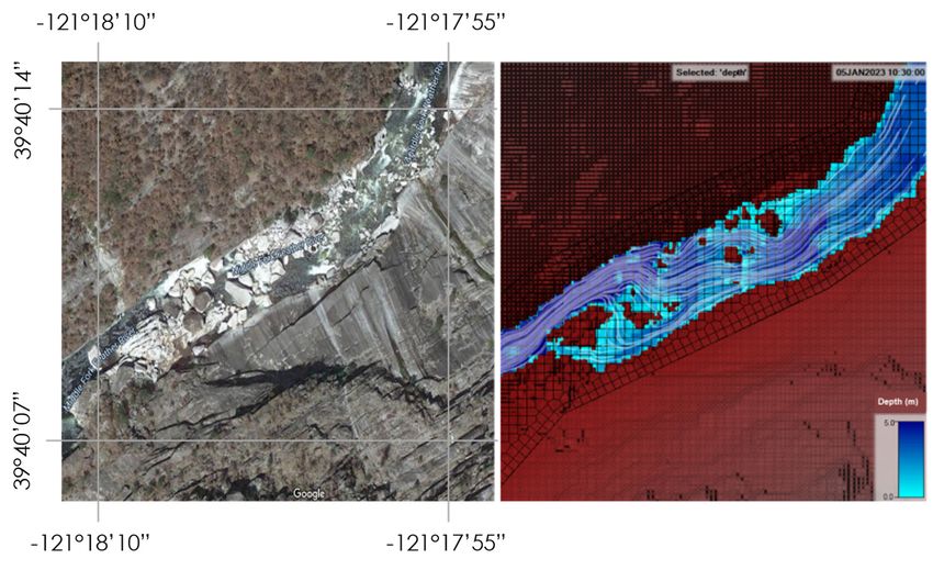
Water 2023, 15, 762                                                                                                                      6 of 23
      Water 2023, 15, x FOR PEER REVIEW                                                                                    6 of 24

                                      Figure 3. LWD extraction and features left behind in the filtering process.
                                     Figure 3. LWD extraction and features left behind in the filtering process.
                                      2.4. Debris Flow Modeling
                                     Table 1. 15-min rainfall intensities over watershed M6 and average recurrence intervals. Data derived
                                          DebrisFlow Predictor (DFP) is an agent-based simulation for shallow debris flows
                                     from the NOAA
                                      and debris      Atlas [14]
                                                 avalanches  14 Point  Precipitation
                                                                  and developed      Frequency
                                                                                  by Stantec    Estimates.
                                                                                             where the details of the model can
                                      be found [26]. It compares favorably to other models [40,41], and provides credible post-
                                                    15-min
                                      wildfire debris        Rainfall
                                                      flow runout      (mm)DFP predicts the flow path,
                                                                    [29,30].                            Average   Recurrence
                                                                                                          the amount  of scourInterval
                                                                                                                               and
                                      deposition along the entire
                                                               8.48path, and the inundation extent of debris flows. Landslide
                                                                                                                       1       pre-
                                      dictions are probabilistic and vary between runs, much as they do in nature. Multiple runs
                                                              10.92                                                    2
                                      allow the user to, therefore, predict the scenario variability across the landscape.
                                                              14.27 along stream segments (produced in the USGS Debris
                                           Debris flow likelihood                                                      5      Flow
                                      Hazard Assessment) within the 13 watersheds was used to establish debris flow initiation
                                                              17.09                                                   10
                                      points for the model scenarios. Stream segments (greater than 0.4 km) with a greater than
                                                              21.08
                                      80% probability of debris   flows for rainfall intensities of 24 mm/h for 15 min25 [38] were
                                                               24.28                                                 50
                                                               27.69                                                100
                                                               31.24                                                200
                                                               36.32                                                500
                                                               40.39                                                1000
Water 2023, 15, 762                                                                                                              7 of 23

                                       Our model scenario established initiation points at locations upstream of all 80%
                                  probability stream segments where the initiation point was established in a location with
Water 2023, 15, x FOR PEER REVIEW
                                  a slope of >30◦ and high burn severity from the North Complex modified BARC                 data
                                                                                                                           8 of 24
                                  (Figure 4). The burn severity value is accepted within the research literature [42,43]. The
                                  slope value is slightly higher than that used by others in the scientific literature but is well
                                  within the range of slopes in which debris slopes initiate [14,44]. A higher slope value was
                                 inconsistency   of sediment
                                  selected to maximize        availability
                                                          debris-flow      alonggiven
                                                                       runout,   manythe
                                                                                       streams, which
                                                                                          disparity     would
                                                                                                    in slope    reduce
                                                                                                             within  thethe avail-
                                                                                                                          medium
                                 ability of thicker  depths of sediment   throughout  the
                                  watersheds and the steep nature of the small watersheds.watershed.

                                Figure
                                 Figure4.4.Debris
                                            Debrisflow
                                                   flowinitiation
                                                        initiationpoints
                                                                   pointsfrom
                                                                          fromwatershed
                                                                              watershedM6
                                                                                        M6(left)
                                                                                           (left)and
                                                                                                  andS1
                                                                                                      S1(right).
                                                                                                         (right).

                                      A five-meter
                                     DFP,            resolution
                                           as a software,  does DEM      was created
                                                                  not identify        and reformatted
                                                                                or specifically          to anLWD
                                                                                                incorporate     ASCII  for use
                                                                                                                    along   the within
                                                                                                                                mod-
                                eled debris flows. The debris flow was therefore assumed to incorporate LWD thatrunout
                                 DFP.  Models   were   calibrated,   run,  and  exported   at this resolution.  Debris   flow    it en-
                                 lengths and
                                countered     deposits
                                           along        wereDebris
                                                   its path.   initially calibrated
                                                                       flow         to estimated
                                                                             pathways,             depths
                                                                                         runout, and       and flow
                                                                                                        debris  dimensions    of recent
                                                                                                                     fan deposition
                                 fans established
                                were  (pre-fire andforpost-fire imagery)
                                                       the scenario.        withinflow
                                                                       The debris   the MF   Feather
                                                                                        fan apex   (theRiver
                                                                                                        upperbased  onofobservations
                                                                                                               extent    the alluvial
                                fan) was determined by where the feeder channel carrying the debris flow began to con-
                                sistently widen proximal to the valley bottom of the MF Feather River.
                                     Only LWD on the ground and readily available for transport were measured. No
                                standing vegetation was measured because of the time required to measure both the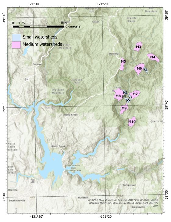
Water 2023, 15, 762                                                                                         8 of 23

                      from Google Earth images and the recent imagery supplied along with the LiDAR data
                      from California Department of Water Resources (CA DWR).
                            Initiation and sediment transport depths along the feeder channels in the watersheds
                      were also calibrated from information gathered in these images. Initial model conditions
                      were set-up based on past expert experience using DFP within this region, as well as
                      testing the model with other known regional debris flows. Landslides were initiated by
                      running the software (Go button) using continuous probabilities (Continuous Function) for
                      debris scour and deposition. Fanning behavior, agent generation, erosion and deposition
                      multipliers, momentum mass loss, and minimum initiation depths (agent settings) were
                      determined in an iterative fashion until the results credibly matched the extent and depth
                      of the historical debris flows and debris flow fans.
                            The final calibrated model settings in DFP contain standard debris flow fan parameters
                      because the fan lengths and widths we assessed in the imagery and slopes measured from
                      DEM data along the MF Feather River are comparable to previously observed debris flow
                      fans we have modeled. Our sediment transport parameters represent a balance between
                      1—the thicker colluvial deposits (>0.5 m) on slopes in the upper watersheds and along
                      some extents of the tributary streams, leading into the MF Feather River; and 2—the thinner
                      layers of colluvium/alluvium (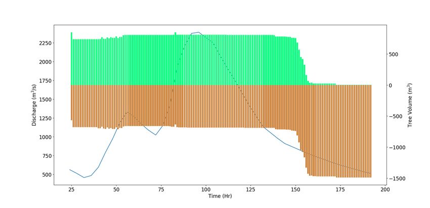
Water 2023, 15, 762                                                                                          9 of 23

                      the expert judgment from other wildfires. Large flow volumes have been shown to entrain
                      and transport large LWD for long distances [17,46]. While there is a large amount of LWD
                      beyond debris flow pathways, studies have shown that much of the LWD associated with
                      debris flows is derived from near the debris flow channel [47].
                            The LWD recorded along the debris flow pathways was randomly placed on the debris
                      flow fan surface in a stratified manner. Debris flows often push LWD at the front of the
                      debris flow surges. When exiting the feeder channel, some of the LWD will be pushed to
                      the lateral extent of the fan (left and right), while the main mass of wood is transported to
                      the distal portion (toe) of the debris flow fan [14,38].
                            The random placement of the wood in the fashion described above required mapping
                      the fan as distinct areas. Debris flow fan perimeters were mapped for each fan. Four
                      areas were identified within each fan perimeter (Figure 5). These areas consisted of two
                      lateral extent areas (roughly where LWD would have been pushed to the lateral extent),
                      the core of the fan (area with the highest probability of a debris flow occupying a raster
                      cell), and the main flow areas in the toe of the debris flow fan (Figure 5). A total of 70%
                      of the LWD from each watershed was randomly placed in the fan toe area and 30% of
                      the total LWD was randomly placed in the two lateral extent areas (10% of the LWD in
                      each) and core of the fan (10% of the LWD) (Figure 5). The decision for the proportionate
                      distribution of the wood on the debris flow fan surface was based on an understanding
                      of flow direction (from the modeling), where sediment mass was transported, and expert
                      judgement from experience at other locations nationally and internationally. Randomly
                      placing the points for the LWD locations in each of the areas was designed to capture the
                      uncertainty in where the LWD would deposit within these fan areas and the ability to
                      cluster the LWD within these locations. The Arcade create random points geoprocessing
                      tool in ArcGIS Pro was used to generate the LWD points within the mapped areas. During
                      the random point generation, the random points generator was permitted to establish
                      zero space between points to simulate depositional clusters of LWD, which is also another
                      common phenomenon evident in LWD transported by debris flows. Upon establishing
                      the random points, x, y coordinates were added to all random points and exported as the
                      coordinates for the LWD tables to be used in the LWD transport modeling.

                      2.5. LWD Transport Modeling
                           For the hydrodynamic simulation, a two-dimensional (2D) hydraulic model was
                      developed using the HEC-RAS model, version 5.0.5 [48]. CA DWR supplied a 2D HEC-
                      RAS model that includes the areas of interest for this analysis [49], hereafter referred to
                      as the Frenchman Dam Model. The Frenchman Dam Model is a 2D HEC-RAS model
                      to understand the flood extent downstream of the Frenchman Dam for two hypothetical
                      failure scenarios: Frenchman Dam failure and Frenchman Spillway weir failure. This model
                      includes the Frenchman Dam, which impounds Frenchman Lake, and the downstream
                      floodplain to Lake Oroville.
Water
Water 2023,
2023, 15,
15, x762
FOR PEER REVIEW 1010ofof24
23
Figure5.
Figure Bins for
5. Bins for randomly
randomly placing
placing LWD
LWD onon the
thedebris
debrisflow
flowfan.
fan.Seventy
Seventypercent
percentofofthe
thepoints
pointsare in
are
the blue area and each remaining area has 10% of the total amount of LWD counted in the
in the blue area and each remaining area has 10% of the total amount of LWD counted in the water-watershed.
shed.
The development of the 2D HEC-RAS model used some modeling parameters from the
Frenchman Dam Model,
2.5. LWD Transport Modelingwith further refinement when necessary. A finer mesh resolution
was required to properly resolve the channel geometry, and the detailed hydrodynamics
For the hydrodynamic simulation, a two-dimensional (2D) hydraulic model was de-
within, rather than just the inundation extent compared with the original model. This
veloped using the HEC-RAS model, version 5.0.5 [48]. CA DWR supplied a 2D HEC-RAS
analysis used a two-stage simulation approach to refine the lateral boundary of the river
model that includes the areas of interest for this analysis [49], hereafter referred to as the
and achieves an optimal balance between model resolution and computational cost. The
Frenchman Dam Model.
model was driven The Frenchman
by the discharge Damupstream,
at the river Model is aand2DaHEC-RAS model of
constant outflow to 289
under-
cms
stand the floodwhich
was applied, extentrepresents
downstream of the Frenchman
a sunny-day Dam
operation, for two hypothetical
as described failure
in the Frenchman
scenarios:
Dam Model. Frenchman Dam failure and Frenchman Spillway weir failure. This model in-
cludesThethemodel
Frenchman
domainDam,
extends which impounds
upstream Frenchman
beyond Lake,
the selected and the downstream
13 watersheds within the
floodplain to Lake Oroville.
MF Feather River where discharge data is available from the USGS gauge near Merrimac.
LakeThe development
Oroville is includedof in
theits2D HEC-RAS
entirety, as themodel
LWD used sometomodeling
are likely parameters
be transported into thefrom
lake.
the
TheFrenchman Damwidth
cross-sectional Model, of with further
the river refinement
is very when
narrow in necessary.
the upper reachAoffiner
the mesh reso-
MF Feather
lution was required to properly resolve the channel geometry, and the detailedof the river and achieves an optimal balance between model resolution and computational
cost. The model was driven by the discharge at the river upstream, and a constant outflow
of 289 cms was applied, which represents a sunny-day operation, as described in the
Frenchman Dam Model.
The model domain extends upstream beyond the selected 13 watersheds within the
Water 2023, 15, 762 MF Feather River where discharge data is available from the USGS gauge near Merrimac. 11 of 23
Lake Oroville is included in its entirety, as the LWD are likely to be transported into the
lake. The cross-sectional width of the river is very narrow in the upper reach of the MF
Feather River, which requires a very high-resolution computational mesh on the order of
River, which requires a very high-resolution computational mesh on the order of 10 ft to
10 ft to adequately resolve the details required for the LWD hydrodynamic transport mod-
adequately resolve the details required for the LWD hydrodynamic transport modeling.
eling.
Theinitial
The initial lateral
lateral boundary
boundary and and
meshmesh resolution
resolution was on
was based based on the Frenchman
the Frenchman Dam Dam
HEC-RAS model. The model was run at 1.5 times the 500-year
HEC-RAS model. The model was run at 1.5 times the 500-year event discharge, and the event discharge, and the
resulting maximum inundation boundary was used to update
resulting maximum inundation boundary was used to update the lateral boundary. This the lateral boundary. This
refinedthe
refined themodel
modelboundary
boundary to to
thethe potential
potential maximum
maximum floodflood extent,
extent, and theandhigh-resolu-
the high-resolution
computational
tion computational cells cancan
cells bebeallocated
allocatedtotoresolve
resolvethe
thenarrow
narrow channel geometry.The
channel geometry. The overall
overall mesh resolution
mesh resolution for different
for different sections
sections of theof the model
model varies
varies from
from 4.64.6
mmatatthe
themost
mostupstream
upstream
reach of thereachMFofFeather
the MF Feather
River toRiver
aboutto 61
about 61 Lake
m for m for Oroville
Lake Oroville
(Figure(Figure 6). The
6). The model has a
model has a total of 102,000 computational
total of 102,000 computational cells. cells.
Mesh
Figure6.6.Mesh
Figure resolution
resolution of the
of the 2D HEC-RAS
2D HEC-RAS hydrodynamic
hydrodynamic model.model.
Thehydrologic
The hydrologic events
events with
with return
return periods
periods of 1, 2,of5,1,25,
2,50,
5, 25,
100,50,
and100,
500and
years500
wereyears were
simulatedwith
simulated withthethe refined
refined 2D 2D HEC-RAS
HEC-RAS hydrodynamic
hydrodynamic model.model. The corresponding
The corresponding dis- dis-
charge
chargeforforthe
theMFMF Feather River
Feather waswas
River obtained from from
obtained the USGS stream stream
the USGS gauge; while
gauge; thewhile the
discharge
dischargefor forother
otherrivers were
rivers derived
were via via
derived a regression
a regressionanalysis usingusing
analysis the available his- histori-
the available
torical discharge records. The regression analysis showed a strong correlation
cal discharge records. The regression analysis showed a strong correlation of the discharge of the dis-
charge
amongamong the rivers
the rivers within within the domain
the domain of interest
of interest with withthethe correlationcoefficient
correlation coefficient for
for the peak
discharge greater than 0.9. Details of the topographical features were resolved, and the
corresponding flow patterns were captured by the model (Figure 7). Although there is no
measured hydrodynamic data for model calibration, the modeling approach follows best
practices, uses the best available information, and has a high mesh resolution.depths and velocity vectors at predefined output time steps from the 2D HEC-RAS model
into the PyLWDSim model; and 2—the function of the inner loop was to calculate the
transport processes of LWD at the much finer time steps required to resolve the transport
processes. This procedure allowed LWD to be simulated with a higher temporal resolu-
tion than hydrodynamics. The hydrodynamic output was at 30-min intervals, while the
Water 2023, 15, 762 time step for the transport process was determined dynamically such that each individual 12 of 23
LWD does not travel more than one mesh cell of the hydrodynamic model grid to ensure
model stability.
(a) (b)
Figure 7. (a) Image of a section of the MF Feather River, (b) an example of the flood depth overlaid
Figure 7. (a) Image of a section of the MF Feather River, (b) an example of the flood depth overlaid
with the velocity streamline from the 2D HEC-RAS model at a rocky section of the MF Feather River
for thethe
with velocity
5-year event.streamline from the 2D HEC-RAS model at a rocky section of the MF Feather River
for the 5-year event.
The recruitment, entrainment, and transport of LWD was hydrodynamically driven.
Flow
The flow depths
depth and and velocity
velocity vectorvectors from the
were needed 2D location
at the HEC-RAS model
of each were
piece used for
of LWD to transport
athe deposited
given LWD
time, since theon the debris flow
hydrodynamics were fancomputed
surface within the at
and saved main
fixedtrunk of the MF Feather
grid locations
River.
from theThe
2D methods
HEC-RASoutlined for the
model. This wasuse of thethrough
achieved LWDSimR modelinterpolation
a bilinear were adopted here [23,50].
using
the
Thehydrodynamic
LWDSimR model outputwas
at the nearest three
converted intomesh nodescode,
a Python that triangulate
which was each LWD. The
coupled directly with
flow depth
the 2D and velocity
HEC-RAS vector
model, at the location
hereafter referredof each
to asLWD were then used
PyLWDSim. Like to determine
[23], the PyLWDSim
the hydrodynamic recruitment, entrainment, and transport process of
and 2D HEC-RAS models were unilaterally coupled ignoring the feedback of LWD on the LWD.
The recruited or downed
the hydrodynamics. trees may beof
The simulation entrained
LWD was in the water column
calculated because
in two nestedof flow.
loops: 1—the
This was determined based on the balance of hydrodynamic (F) and resistance forces (R)
function of the outer loop was to load the hydrodynamic results in terms of flow depths
and velocity vectors at predefined output time steps from the 2D HEC-RAS model into the
PyLWDSim model; and 2—the function of the inner loop was to calculate the transport
processes of LWD at the much finer time steps required to resolve the transport processes.
This procedure allowed LWD to be simulated with a higher temporal resolution than
hydrodynamics. The hydrodynamic output was at 30-min intervals, while the time step for
the transport process was determined dynamically such that each individual LWD does not
travel more than one mesh cell of the hydrodynamic model grid to ensure model stability.
The recruitment, entrainment, and transport of LWD was hydrodynamically driven.
The flow depth and velocity vector were needed at the location of each piece of LWD for
a given time, since the hydrodynamics were computed and saved at fixed grid locations
from the 2D HEC-RAS model. This was achieved through a bilinear interpolation using
the hydrodynamic output at the nearest three mesh nodes that triangulate each LWD. The
flow depth and velocity vector at the location of each LWD were then used to determine
the hydrodynamic recruitment, entrainment, and transport process of the LWD.
The recruited or downed trees may be entrained in the water column because of flow.
This was determined based on the balance of hydrodynamic (F) and resistance forces (R)
on individual LWD pieces according to [51]. With the assumption that each LWD piece was
positioned perpendicular to the flow direction, the hydrodynamic force F can be written as
1
F= C ρkdhU 2 (1)
2 d
where Cd is the drag coefficient for the LWD in water, ρ is the density of water, d is the
diameter of the LWD, h is the flow depth, U represents velocity magnitude, and the lengthWater 2023, 15, 762 13 of 23
of the LWD is expressed as l = kd. The density of the wood element is assumed to be close
to that of water. The resistance forces can be estimated as
2
πd
R = gρkdµ − Asub (2)
4
where g is gravitational acceleration, µ is the friction coefficient between the LWD and the
channel bed, and the submerged area of the log perpendicular to its length can be defined as
2 1 −1 2h 1 −1 2h
Asub = d cos 1− − sin 2cos 1− (3)
4 d 8 d
The balance between the hydrodynamic force and resistance force can then be ex-
pressed using a non-dimensional factor as
1
F C hU 2
Ψ= = 2 2d (4)
R gµ πd4 − Asub
The condition that yields the balance of the hydrodynamic and resistance force, i.e.,
Ψ = 1, is the critical condition, and the threshold velocity for the movement of the LWD is
then expressed as
s
gµd2
2h 1 2h
Ulim = π − cos−1 1 − + sin 2cos−1 1 − (5)
2Cd h d 2 d
The following simplified scheme was considered according to [52]:
Case I: If h > d, the LWD piece is floating, with the associated transport inhibition
parameter c = 0.
Case II: If h < d, and 0 < U < Ulim , the LWD piece is resting, with the associated
transport inhibition parameter c = 1.
Case III: If h < d, and U > Ulim , the LWD piece is either rolling or sliding, with the
associated transport inhibition parameter expressed as
h
c = 1− (6)
d
and the velocity along the transport trajectory for each moving LWD piece is estimated
as follows:
U LWD = (1 − c)U (7)
The transport velocity can then be used to calculate the new position for every trans-
ported LWD at each time step. A moving LWD piece can be deposited at a particular
time step if the conditions for entrainment were no longer fulfilled, and the LWD can be
remobilized in a subsequent time step.
The model parameters were specified in the text input file, which includes the project
description path to the 2D HEC-RAS output HDF file; the hydrodynamic basin name
defined in the 2D HEC-RAS model; the output time interval for hydrodynamics results; the
starting time for LWD transport modeling in terms of the number of hydrodynamic output
time intervals, such that the hydrodynamic model is stable; the LWD transport modeling
duration in terms of number of hydrodynamic output time intervals; the path to LWD
input; and the path to the output folder. The LWD input was a CSV file containing the
following information for each recruited LWD piece from the debris flow predictor model:
• ID: Unique identifier for each LWD as a sequential integer.
• Watershed: The name of the watershed where the LWD originates.
• Xcoord and Ycoord: The initial x- and y-coordinate of the LWD in the debris flow
fan areas.Water 2023, 15, 762 14 of 23
• DBH: The diameter of the LWD piece at breast height.
• Status: Status of the tree, which is classified as 1 = rooted, 2 = lying, 3 = moving,
4 = jammed. The initial status of living wood is always 1 and that of dead wood is 2.
• Rootwad: The diameter of Rootwad of the LWD piece.
• Length: The length of the LWD piece.
• Structure: The wood structure for a standing tree.
• Slope: The geomorphologic characteristics of the areas for the LWD of piece.
The model output contained the location, status, characteristics, and hydrodynamics
of all LWD pieces at every five timesteps to allow for a detailed understanding of the
temporal transport dynamics. The output data were used in post-processing to determine
the transport path and fate of the LWD at any time during the simulation.
The fate of the LWD was also analyzed to understand the volume of LWD and the
corresponding transport ratio of the LWD, defined as the mobilized or relocated volume
of LWD at any given time (or the volume of LWD that reach Lake Oroville at the end of
simulation as a special case) to the total available LWD from the debris flow model. The
relatively narrow river cross-section width of the MF Feather River, which was comparable
to the length of some large LWD, especially within the upper reaches of the MF Feather
River required an adjustment to be made to the transport ratio from the model output.
The adjustment to the transport ratio addresses a model limitation whereby the dimension
of the LWD was not accounted for throughout the LWD transport along the MF Feather
River and ultimately provided a more realistic simulation of the LWD fate. For each LWD
transported along the MF Feather River, the length of the LWD was compared with the
most critical cross-section (narrowest width) downstream from its origin. Should the length
of the LWD be greater than the critical width, the LWD was removed from the account. The
transport ratio was then recalculated with the remaining LWD to mimic sorting of LWD
along the flow pathway towards Lake Oroville.
For each hydrologic event, the transport ratio of LWD was defined as the volume of
LWD that reached Lake Oroville from a watershed to the total initial volume of LWD within
that watershed, as well as the total transport ratio accounting for all LWD in all watersheds.
The transport ratios were calculated directly using the model output, which was identified
as ‘no adjustment’. They were also calculated by removing the pieces with a length greater
than the critical cross-section width of the river, following the approach discussed in the
Sub-Scenario of the LWD Transport Modeling, which was identified as ‘adjusted’.
3. Results
3.1. LWD Transport via Debris Flows
A total of 1073 pieces of LWD potentially would be transported via debris flows from
the 13 modeled watersheds to the MF of the Feather River. The small watershed had
lesser debris flow volumes (Table 2). Medium watersheds produced a total of 889 pieces of
LWD compared with 116 pieces of LWD from the small watersheds. Medium watersheds
produce 111 pieces of LWD on average (range was 13 to 194 pieces of LWD), while the
small watersheds produced 37 pieces of LWD on average (range was 7 to 81 pieces of LWD).
Small watersheds produced more LWD than some of the medium watersheds despite
possessing 12 the drainage area of most of the medium watersheds. There was a weak
positive trend between the debris flow volume and the LWD volume (Table 2). All LWD
volumes were below 1% of the debris flow volumes except for watershed M3, which was
an outlier making up 5% of the total volume.Water 2023, 15, 762 15 of 23
Table 2. LWD counts and volumes from each watershed.
Watershed Number Hectares LWD Count LWD Volume (m3 ) Debris Flow Volume (m3 )
M3 204.6 144 517.6 9181.4
M4 235.7 140 430.4 92,075.4
M5 176.1 33 103.5 107,562.6
M6 303.0 194 380.1 971,462.7
M7 243.5 139 451.4 379,752.3
M8 375.5 83 132.4 129,475.8
M9 202.0 13 24.5 147,622.5
M10 222.7 143 644.1 577,597.5
S1 62.2 81 153.6 284,825.7
S2 46.6 9 11.5 76,653.0
S3 20.7 17 118.0 64,341.0
S4 5.2 7 2.3 41,096.7
S5 77.7 70 190.0 228,922.2
Total 2175.6 1073 3159.4 3,110,568.8
Small Sum 212.4 184 475.4 695,838.6
Medium Sum 1963.2 889 2684.0 2,414,730.2
Small Mean 42.5 36.8 95.1 139,167.7
Medium
Water 2023, 15, MeanREVIEW
x FOR PEER 245.4 111.1 355.5 301,841.3
16 of 24
3.2. LWD Transport and Fate along the MF of Feather River and into Lake Oroville
The transport
The temporalratio LWD
of LWD increased
transport with anwere
dynamics increasing return
illustrated period,
as the volume which was that
of LWD
expected as higher
mobilized versusdischarge
the volumecauses greater
of LWD depth, flow
that deposited for avelocities,
given timeand transporting
during the simulation
power(Figure
(Table8).3). A significant
Few LWD were amount of LWD
transported was
into mobilized
Lake Orovillewithin
duringthethefirst fewevent.
1-year time steps
LWDs ofstarted
the simulation and sometodeposition
to be transported was observed
Lake Oroville during thealong theevent,
2-year bankswhere
of thethe
river. As the
total
discharge
transport increased,
ratio was newtoand/or
estimated previously
be 9% to 25%, withdeposited
and without LWD were mobilized.
adjustment (Table 3).During
The the
falling
transport limb
ratio of the hydrograph,
increased especially
to 46% to 58% for the at the tail event
500-year end, mobilized
(Figures 11LWDandwere
12). transported
downstream and eventually deposited after reaching the lower boundary of the model at
the dam.
FigureFigure 8. Temporal
8. Temporal LWD LWD transport
transport dynamics
dynamics against
against the hydrograph
the hydrograph for50-year
for the the 50-year
event.event.
The spatial distribution of LWD was first analyzed using a raster that shows the
volume of LWD passing through a fixed raster cell at a resolution of 3 m, referred to as the
transport path volume raster. Figure 9 shows the flow path volume raster for the 50-yearWater 2023, 15, 762 16 of 23
event. The transport path was concentrated along the main channel of the river, especially
for the upper reach of the MF Feather River, but spread after reaching the wider section
at the lower reach adjacent to Lake Oroville. The transport path eventually ended along
the dam with LWD deposited near the entrance of spillway. The effects of wind and the
corresponding surface flow that may further spread the LWD within Lake Oroville were
not considered
Figure in the
8. Temporal LWD LWDdynamics
transport transport modeling.
against the hydrograph for the 50-year event.
Figure 9. Flow path volume raster for the 50-year event.
Figure 9. Flow path volume raster for the 50-year event.
Most of the LWD ends up in Lake Oroville (Figures 9–12), some LWD were trapped
within the MF Feather River (Figure 10). LWD also remained at their initial location as the
flow did not reach the full extent of the debris flow fan surface, especially for watersheds
M3, M5, and M10, which are located at small branches of the MF Feather River with much
smaller discharges. LWD was deposited near the banks approaching river bends or after
Water 2023, 15, x FOR PEER REVIEW 17 of 24
cross-section expansion (Figure 10). LWD was also trapped at locations with large bed
rocks (Figure 10).
Figure 10. Potential deposition locations for LWD within the MF Feather River. (a) LWD deposited
Figure 10. Potential deposition locations for LWD within the MF Feather River. (a) LWD deposited on
on meander bend and island. (b) LWD trapped above flow height and along banks entering a me-
meander bend
ander. (c) and
LWD island.
trapped on (b) LWD
islands trapped
and in areasabove
whereflow height expands
the channel and along banks
at the entering
lateral extent. a(d)
meander.
LWD trapped on rocks.
(c) LWD trapped on islands and in areas where the channel expands at the lateral extent. (d) LWD
trapped on rocks.Figure
Figure10.
10.Potential
Potentialdeposition
depositionlocations
locationsfor
forLWD
LWDwithin
withinthe
theMF
MFFeather
FeatherRiver.
River.(a)
(a)LWD
LWDdeposited
deposited
on
on meander bend and island. (b) LWD trapped above flow height and along banksentering
meander bend and island. (b) LWD trapped above flow height and along banks enteringaame-
me-
Water 2023, 15, 762 ander. 17 of 23
ander.(c)
(c)LWD
LWDtrapped
trappedononislands
islandsand
andininareas
areaswhere
wherethe
thechannel
channelexpands
expandsatatthe
thelateral
lateralextent.
extent.(d)
(d)
LWD
LWDtrapped
trappedononrocks.
rocks.
Figure 11.
Figure11. The
11.The total
Thetotal transport
totaltransport ratio
transportratio ofofLWD
ratioof as
asaaafunction
LWDas function ofofhydrologic
functionof event
hydrologicevent return
eventreturn periods.
returnperiods.
periods.
Figure LWD hydrologic
Figure 12.
Figure12. The
12.The transport
Thetransport ratio
transportratio for
ratiofor each
foreach individual
eachindividual watershed
individualwatershed for
watershedfor the
forthe 50-year
the50-year event.
50-yearevent.
event.
Figure
The transport ratio of LWD increased with an increasing return period, which was
expected as higher discharge causes greater depth, flow velocities, and transporting power
(Table 3). Few LWD were transported into Lake Oroville during the 1-year event. LWDs
started to be transported to Lake Oroville during the 2-year event, where the total transport
ratio was estimated to be 9% to 25%, with and without adjustment (Table 3). The transport
ratio increased to 46% to 58% for the 500-year event (Figures 11 and 12).Water 2023, 15, 762 18 of 23
Table 3. Summary of LWD transport ratio to the available LWD volume at each watershed.
LWD Volume Transport Ratio—No Adjustment
Watershed
Volume (m3 ) Ratio 1-Year 2-Year 5-Year 25-Year 50-Year 100-Year 500-Year
M3 264 0.16 0 0 0 0 0.08 0 0.36
M4 219 0.14 0 0.17 0.97 0.98 0.98 0.98 1
M5 53 0.03 0 0 0 0.06 0.05 0.33 0.56
M6 194 0.12 0 0.45 0.66 0.74 0.86 0.89 0.91
M7 230 0.14 0 0.55 0.8 0.75 0.75 0.67 0.68
M8 67 0.04 0 0.6 0.55 0.62 0.62 0.67 0.67
M9 12 0.01 0.35 0.35 0.35 0.35 0.35 0.35 0.35
M10 328 0.2 0 0 0 0 0 0 0
S1 78 0.05 0 0.03 0.66 0.89 0.93 0.93 0.95
S2 6 0 0 0.2 0.63 0.63 0.63 0.63 0.63
S3 60 0.04 0 0.99 0.74 0.74 0.74 0.74 0.74
S4 1 0 0 0.87 0.85 0.87 0.87 0.87 0.91
S5 97 0.06 0 0.39 0.4 0.63 0.64 0.8 0.81
Total 1609 1 0 0.25 0.44 0.47 0.5 0.51 0.58
LWD Volume Transport Ratio—Adjusted
Watershed
Volume (m3 ) Ratio 1-Year 2-Year 5-Year 25-Year 50-Year 100-Year 500-Year
M3 264 0.16 0 0 0 0 0 0 0.01
M4 219 0.14 0 0.05 0.45 0.46 0.65 0.65 0.8
M5 53 0.03 0 0 0 0.03 0.02 0.01 0.01
M6 194 0.12 0 0.24 0.48 0.74 0.86 0.89 0.91
M7 230 0.14 0 0.17 0.46 0.56 0.56 0.48 0.66
M8 67 0.04 0 0.34 0.33 0.62 0.62 0.67 0.67
M9 12 0.01 0.35 0.35 0.35 0.35 0.35 0.35 0.35
M10 328 0.2 0 0 0 0 0 0 0
S1 78 0.05 0 0.03 0.28 0.65 0.69 0.69 0.95
S2 6 0 0 0.2 0.63 0.63 0.63 0.63 0.63
S3 60 0.04 0 0.08 0.33 0.33 0.33 0.33 0.33
S4 1 0 0 0.87 0.85 0.87 0.87 0.87 0.91
S5 97 0.06 0 0.14 0.39 0.55 0.56 0.56 0.81
Total 1609 1 0 0.09 0.25 0.34 0.38 0.39 0.46
3.3. Comparison to Previous LWD Removals from Lake Oroville
Historically, LWDs within Lake Oroville had been removed on an annual basis during
most years when regular storms occurred. The intensity of the storms was not documented,
but the removed LWD were placed on a pile with an area of 10 hectares and a height
typically reaching 1.21 m for most years and less for others. The debris was not collected
in 2022 due to the lack of storms, as communicated by CA DWR. The packing ratio of the
wood pile, defined as the ratio of wood volume to the total pile volume, ranges from 0.06 to
0.26, which can be higher for clean piles with larger logs [53]. Assuming a packing ratio of
0.25, the removed LWD volume was estimated as
10 hectares × 1.21 m × 0.25 = 30, 837 m3
The selected 13 watersheds with past wildfires had a total drainage area of 21 sq
km, while the total burned area for the North Complex Fire was 1191 sq km. Using the
estimated total volume of LWD from the 13 watersheds and the transport ratio from the
PyLWDSim model, the total volume of LWDs from all burned watersheds that enter Lake
Oroville can be estimated with a simple extrapolation based on the ratio of the drainage area
(Table 4). Since the previous removals occurred for most years but not all, it is reasonable
to compare that to high frequency events such as a 2-to-5-year event, where the estimatedWater 2023, 15, 762 19 of 23
total transported volume of LWDs in Lake Oroville ranges from 274 m3 to 42,141 m3 with
adjustment and 274 m3 to 53, 467 m3 without, which was consistent with the estimated
historical removal volume.
Table 4. Extrapolated transport volume of LWD in Lake Oroville from all burned watersheds.
LWD Volume (m3 )
Return Period (Years)
Adjusted No Adjustment
1 274 274
2 8428 22,807
5 23,480 40,503
25 31,456 46,716
50 35,505 46,374
100 36,823 47,355
500 42,141 53,467
4. Discussion
The LWD transport modeling showed the potential for a major portion of the LWD
available arriving in Lake Oroville for both the LWD jam and non-jam scenarios. Consistent
with previous research [4], our model results showed the largest volume of LWD trans-
ported to Lake Oroville was associated with the largest flood. In our LWD jam modeling
scenario the 5-year event transports 25% of the LWD brought to the MF Feather River via
debris flows to the reservoir. The 25-year, 50-year, and 100-year flood events fall within
the range of 34% to 39% (increasing with flood magnitude) indicating that floods with
these return intervals have the potential to transport significant amounts of LWD to Lake
Oroville. Some watersheds did not have strong connectivity with the MF Feather River
or did not have significant volumes of LWD transported to the debris flow fans. The
watersheds with higher connectivity often exhibit transport ratios greater than 60%, with
several watersheds (five in total) with transport ratios greater than 80%. The differences in
connectivity are likely representative of what is happening within the system and reflect
our current understanding of connectivity [53].
The above numbers also highlight that not all LWD was transported to the reservoir.
Some of the tributaries that did not have high connectivity with the MF of the Feather River
were small systems that did not produce discharges to transport the LWD to the mainstem
river. Entrained LWD not arriving at the reservoir was often deposited and stored on
mid-channel bars, trapped by large boulders in the channel, deposited at the beginning of
an outer bend of a meander, or deposited in reaches where the channel width expanded.
These findings support previous work that shows LWD jams in similar locations within
another region of California [5]. In other instances, LWD was also not entrained from the
debris flow fan surfaces, as the flood elevation was not high enough to entrain the LWD
located outside of the flood extent. As no bridges were present along the mainstem river,
these structures did not play a significant role in trapping LWD being transported along
the MF Feather River, as has been identified in previous studies [17].
The debris flow modeling, while critical to the understanding the LWD transport
from tributaries to the mainstem streams, also highlights the importance of sediment
transport from this process. Sediment transport was not a component of this study along
the MF Feather River. However, inferences can be made given our observations and
previous experience. Analysis of the canyon section of the MF Feather River shows limited
sediment storage. Major portions of the debris flow fan deposits would be transported
along with the LWD during flooding. This has implications for the MF Feather River, as
large particles transported by the debris flows will likely be left behind in the vicinity of
the debris flow fan to form rapids. Should rocks within these areas protrude through or
be close to the water surface, these might serve as potential locations for trapping LWDWater 2023, 15, 762 20 of 23
from upstream. Sediment transported from the debris flow fans can change downstream
channel morphology through the development of new bars or the expansion of existing
bars (lateral, mid-channel, and point bars). There is also the potential for transporting
large amounts of sediment from the debris flow fans to the reservoir during a flood, as on
average the modeled debris flow fans had 695,830 m3 of material stored in them.
The models were based on some simplifications and assumptions. We attempted to
reduce the epistemic uncertainty from not knowing or not having information available to
resolve all the potential dynamics within the systems. In the debris flow modeling multiple
predictive simulations and probabilistic approaches were used to reduce uncertainty and
enhance our ability to represent the system dynamics. The debris flow model represents
our best effort to identify the locations and magnitudes of credible scenarios for debris flow
initiation, runout, and inundation. Despite the diligence, the following are limitations to
our modeling approach for the debris flow transport of LWD:
• Debris flow fan development was impacted by the lack of LiDAR data in the channel of the
MF Feather River. The faceted DEM at this location had an impact of debris flow formation
and these represent a best approximation of the surficial feature at these locations.
• There were heavily burned standing trees along the channels that were not incorpo-
rated into the counts of LWD. These could become a potential source of LWD as they
fall into channels through the undercutting of the stream bank, wind throw, or as the
trees decompose over time. These will continue to provide a supply of LWD to the
system over time.
• There were locations along the watershed valley bottoms where LWD sampling was
inhibited by “noisy” LiDAR data associated with dense lower canopy vegetation and
in some instances these areas were in shadows within the imagery because of the time
of day the aerial photographs were taken. In both instances, the LWD population
through these areas was likely underrepresented.
• We assumed entrained LWD in our modeling approach made it out of the medium
and small watersheds to the MF Feather River. This was a limitation in the approach,
as we were unable to account for terrain conditions where the LWD might have been
trapped behind large rocks or jammed behind trees and between the banks. This
could lead to an overestimation of the amount of LWD from the ground that would
be transported to the MF Feather River. However, even with this limitation, we were
likely underestimating the total magnitude of LWD because the burned standing trees
are not accounted for in this measurement.
Similarly, there are limitations to the LWD transport modeling. The transport dy-
namics and fate of the LWD within the Lake Oroville watersheds were studied using the
PyLWDSim model based on previous methods [50] where the hydrodynamics were derived
using the 2D HEC-RAS model. There are some limitations intrinsic to the data availability,
model assumption, and simplification that may affect the accuracy of the analysis.
• The hydrodynamics were derived using the 2D HEC-RAS model, where the following
limitations for the application to the hydrodynamic transport of LWD were identified:
• The hydrodynamic was resolved at the resolution of the bathymetry data.
• The hydrodynamic model lacked validation due to limited data although the best
practices were followed for model setup, parameterization, etc.
• The influence of wind on the surface velocity was not included in the hydrodynamic
model where the resulting surface flow can change the path of the LWD within
Lake Oroville.
• The hydrodynamic was unilaterally coupled with the transport model such that the
influence of the LWD on the hydrodynamics is not accounted for. This may have
resulted in poor results where the river channels were jammed by LWD.
• The hydrodynamic transport of LWD was a very complex process involving LWD
recruitment due to the hydro-dynamic, entrainment, transport, and deposition of
LWD, and obstruction of LWD.You can also read


