ACTIVITY-BASED AND AGENT-BASED TRANSPORT MODEL OF MELBOURNE (ATOM): AN OPEN MULTI-MODAL
←
→
Page content transcription
If your browser does not render page correctly, please read the page content below
Activity-based and agent-based Transport model
                                                       of Melbourne (AToM): an open multi-modal
                                                              transport simulation model for Greater
arXiv:2112.12071v1 [physics.soc-ph] 16 Dec 2021

                                                                                         Melbourne
                                                   Afshin Jafari* a , Dhirendra Singhb,c , Alan Botha , Mahsa Abdollahyara ,
                                                          Lucy Gunna , Steve Pembertona , and Billie Giles-Cortia
                                                       a
                                                           School of Global, Urban and Social Studies, RMIT University
                                                              b
                                                                School of Computing Technologies, RMIT University
                                                                                c
                                                                                  Data61, CSIRO

                                                                                       December 23, 2021

                                                                                                 Abstract

                                                              Agent-based and activity-based models for simulating transportation systems
                                                           have attracted significant attention in recent years. Few studies, however, include
                                                           a detailed representation of active modes of transportation—such as walking and
                                                           cycling—at a city-wide level, where dominating motorised modes are often of pri-
                                                           mary concern. This paper presents an open workflow for creating a multi-modal
                                                           agent-based and activity-based transport simulation model, focusing on Greater
                                                           Melbourne, and including the process of mode choice calibration for the four main
                                                           travel modes of driving, public transport, cycling and walking. The synthetic pop-
                                                           ulation generated and used as an input for the simulation model represented Mel-
                                                           bourne’s population based on Census 2016, with daily activities and trips based on
                                                           the Victoria’s 2016-18 travel survey data. The road network used in the simulation
                                                           model includes all public roads accessible via the included travel modes. We com-
                                                           pared the output of the simulation model with observations from the real world in
                                                           terms of mode share, road volume, travel time, and travel distance. Through these
                                                           comparisons, we showed that our model is suitable for studying mode choice and
                                                           road usage behaviour of travellers.
                                                     * Corresponding
                                                                  Author. Email address: afshin.jafari@rmit.edu.au. Postal address: RMIT University,
                                                  GPO Box 2476, Melbourne VIC 3001.

                                                                                                    1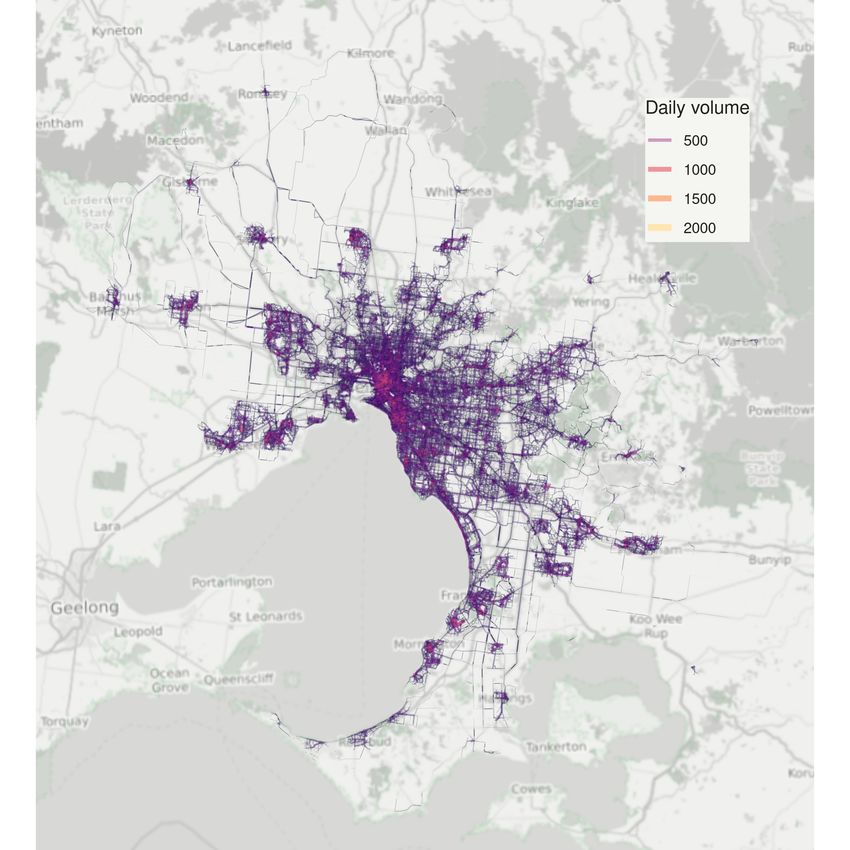
1    Introduction
Computer-based transport simulations have been used for more than five decades to
inform transport system management and decision-making (McNally, 2007). The tra-
ditional approach to building transport simulation modelling was to divide the system’s
behaviour into four main steps: (i) trip generation (how many trips?); (ii) trip dis-
tribution (between which zones?); (iii) modal split (using which travel modes?); and
(iv) assignment (via which routes?). Although four-step models have paved the way for
the widespread use of simulation in planning for transport systems, a key limitation is
their inability to associate trips to individuals and consequently to capture the hetero-
geneous behaviours of travellers, interactions between them, and inter-dependencies
between different components of the transport system (e.g., infrastructure, conges-
tion, travellers’ mode and route preferences and trip chains) (Rasouli and Timmermans,
2014).
    Activity-based modelling of transport systems addresses many of the four-step
models’ shortcomings through a dis-aggregated approach involving modelling indi-
viduals and their trips, activities, and heterogeneous decision-making and behaviours
(McNally and Rindt, 2007; Rasouli and Timmermans, 2014). Activity-based models
take a bottom-up approach and simulate the individual behaviour of each entity of the
system, the interactions between entities as well as with the environment (Kagho et al.,
2020). From this perspective, the disaggregated approach of activity-based modelling
is congruent with Agent-Based Models (ABMs) that are computational models of het-
erogeneous agents and their interactions within their environment that can be used
for experimenting with different possible scenarios (Gilbert, 2021). Thus, significant
benefit could be derived by joining the two approaches to capture both heterogeneous
travel plans and complex interactions between travellers (Tajaddini et al., 2020; Hörl
and Balac, 2020a).
    Multi-Agent Transport Simulation (MATSim) is an open-source transport simula-
tion toolkit that provides this link between agent-based and activity-based models and
has become popular for large-scale transport models over the last decade (Horni et al.,
2016; Hager et al., 2015). MATSim is designed and optimised for large-scale simula-
tions, which makes it a suitable option for city-wide models. Notable examples of the
development of large-scale MATSim models include Switzerland (Bösch et al., 2016),
Singapore (Erath et al., 2012), Melbourne (Infrastructure Victoria, 2017), while more
recent models include those for Paris (Hörl and Balac, 2020b) and Berlin (Ziemke
et al., 2019a). Furthermore, MATSim has been used to model different aspects of the
transport system including Public Transport (PT) (Rieser, 2016), cycling (Ziemke et al.,
2019b), and novel concepts such as shared mobility (Becker et al., 2020) and shared
autonomous electric vehicles (Müller et al., 2021).
    Another important trend in modelling the transport system of cities is the move

                                           2
towards multi-modal agent-based and activity-based models rather than the traditional
approach of modelling only car and PT. For example, Oh et al. (2020) analysed the
impact of automated mobility-on-demand services using a multi-modal agent-based
model for Singapore. The agent-based model Chapuis et al. (2018) model for flood
emergency management for Hanoi, Vietnam, is another example of large-scale multi-
modal simulation models. Despite the rise in multi-modal simulation models of cities,
developing such models is a complicated and involved process and omitted to date is a
flexible process for creating large-scale active transport simulation models using open
data and tools.
     In this paper, we present our work on building a large-scale simulation model of
the transport system for Greater Melbourne, Australia. Our model is based on MAT-
Sim simulation toolkit and is the first multi-modal calibrated and open1 activity-based
MATSim model for Melbourne. With this model, we aim to fill the gap of multi-modal
open large-scale models in the literature and to use it as a baseline model for future sim-
ulation studies of Melbourne’s transport system with a focus on active transport (i.e.,
walking, cycling and PT). Furthermore, the complete workflow of producing the model
as well as the tools we developed as part of the process are available on GitHub2 with
the aim of addressing the need for flexible tools and processes for creating large-scale
simulation models for active transport.
    The remainder of this paper is laid out as follows. Section 2 provides an overview
of the key concepts in building activity-based transport models using the MATSim
simulation toolkit. Section 3 describes our workflow and the key tools and methods
used to develop the simulation model for Melbourne. The calibration process of the
model and evaluation of the calibrated scenario are discussed in Section 4. Finally, in
Section 5 we discuss how this model could be used to help inform decision-making
for the transport system in Melbourne, and the applicability of the framework to other
cases and potential future steps of the model.

2      Background
The three main building blocks of an ABM are: (i) a synthetic population of hetero-
geneous agents; (ii) their environment; and (iii) a way for agents to interact with each
another and their environment (Wall, 2016). For transport system ABMs, the synthetic
population is a list of travellers, their attributes, and their travel diaries. Different ap-
proaches to build synthetic populations for transport modelling are briefly reviewed in
Section 2.1. The environment for transport ABMs is typically the road network that the
    1 We note that the first calibrated activity-based MATSim model for Melbourne was MABM (Infrastruc-
ture Victoria, 2017). Ours is the first calibrated multi-modal model that is also open. We also use more recent
census and VISTA data than MABM.
    2 https://github.com/matsim-melbourne

                                                      3
agents use to travel to their daily destinations. Section 2.2 reviews recent studies for
creating road network models for ABMs. Lastly, we used MATSim as our ABM simu-
lation framework to model the transport system. Section 2.3 briefly discusses MATSim
and how it models the interaction amongst agents and their environment.

2.1    Synthetic population construction
Synthetic population generation based on the activity-based modelling framework typ-
ically involves steps for generating a list of agents with their demographics, assigning
activity patterns (i.e., activity chain or itinerary), and assigning locations to activities
(Wang et al., 2021). Over the years, a number of different methods have been devel-
oped to produce the synthetic population for activity-based and agent-based transport
models.
    A widely used approach is to create a synthetic population based on probability
distributions from travel surveys. For example, Travel Activity Scheduler for House-
hold Agents (TASHA), a well-known travel demand generator calibrated for Greater
Toronto Area (Roorda et al., 2008), uses a joint probability distribution function for cre-
ating activity-based travel demands. In TASHA, population and demographics repli-
cate Greater Toronto’s transport survey, representing 4.5% of the population. The sur-
vey was also used to create joint probability functions for different activity types, de-
mographics, household structure, and trip schedules, resulting in 262 distributions that
were used to generate activities. A similar probabilistic approach was also used to se-
lect the activity start time and duration for each activity. These functions were then used
to generate the list of activities of each individual. Home and work locations in TASHA
were given to the model as inputs and locations for other activities were assigned us-
ing entropy models based on distance, employment density, population density, and
measures for other land-use types such as shopping mall floor space for the shopping
activity (Roorda et al., 2008).
    More recently, machine learning techniques have been used to enhance synthetic
population generation accuracy and flexibility (Koushik et al., 2020). For example,
Hesam Hafezi et al. (2021) used techniques from machine learning along with econo-
metric techniques and proposed a hybrid framework for creating activities and travel
diaries using a cohort-based synthetic pseudo panel engine to model. Similarly, a k-
means clustering algorithm was used by Allahviranloo et al. (2017) to cluster activities
based on trip attributes and to synthesize activity chains.
    Both et al. (2021) proposed an algorithm for creating the synthetic population for
the Greater Melbourne area using a combination of machine learning, probabilistic and
gravity-based approaches. In their algorithm, each synthetic individual was assigned
a demographic profile (e.g., age, gender) consistent with the census population at the

                                             4
Statistical Area level 2 (SA2) geospatial boundary,3 a home location (i.e., a valid street
address in that SA2), and a daily travel plan comprising a sequence of activities (at par-
ticular locations and times of the day) connected by travel legs (using particular modes,
e.g., driving, PT) consistent with the travels observed for persons of that demographic
profile in the Victorian Integrated Survey for Travel and Activity (VISTA) 2012-18
travel survey data (Department of Transport, 2018).
      Five destination types of home, work, education, commercial, and park were in-
cluded in the algorithm. The destinations of different types were distributed across
Greater Melbourne based on the Vicmap Address database by the Victorian govern-
ment4 containing 2,932,530 addresses and their Mesh Block (MB) land use categories.
MB is the smallest geographical area defined by ABS and residential MBs have a
dwelling count of approximately 30 to 60 in urban areas.5 Both et al.’s algorithm also
assigns a travel mode to each trip based on the starting region’s probability to be used
for the location assignment process (Both et al., 2021).
    When assigning locations to activities, the assigned transport mode, the distance
traveled to the destination, and the destination itself for the activity were required to
account for local variation while also conforming to global distributions. To ensure this
was the case, for each SA1 region, values were calculated based on the VISTA travel
survey. New locations were chosen sequentially for each agent, with the restriction that
agents start and finish at home. Transport mode was chosen first, so that the candidate
regions can be filtered down to the ones likely for that mode, based on the number of
trips remaining to get home. This was to ensure that the final trip home will not be un-
reasonably long. The remaining regions were then ranked based on their distance and
how likely the agent would be to choose the region based on the local distance distribu-
tion and the attractiveness of that region for the specified location type. Additionally,
global distance distribution and destination attraction were considered to ensure that
the synthetic population’s overall trip length and destination choice reflected that of
the VISTA travel survey. Figure 1 illustrates how the distance distribution and trans-
port mode probabilities, and destination type probabilities were combined to create the
probabilities needed to select the next region.

2.2     Road network model construction methods
One of the main inputs of the transport simulation models is the road network descrip-
tion. This not only indicates the location of the road infrastructure that agents can travel
through, but also assesses its quality and usage specifying, for example, road capac-
   3 Demographic distributions were matched to Australian Bureau of Statistics (ABS) Census 2016 at the
SA2 geospatial boundary, which conceptually represents a community of on average 10,000 persons.
  4 https://discover.data.vic.gov.au/dataset/address-vicmap-address
  5 https://www.abs.gov.au/ausstats/abs@.nsf/Lookup/by%20Subject/1270.0.

55.001˜July%202016˜Main%20Features˜Mesh%20Blocks%20(MB)˜10012

                                                  5
(a)                                        (b)

                     (c)                                        (d)

                     (e)                                        (f)

Figure 1: Selecting next region for a cycling trip from home (circle) to work (triangle)
showing: region selection probability (Pr) for local and global distance distributions (a
and b), region selection probability (Pr) for local and global destination attraction (c
and d), number of trips (hop count) that would be reasonably required to reach home
(e), and combined region likelihood (f) (source: (Both et al., 2021)).

                                           6
ity and speed limits, and what modes are allowed on particular roads. In other words,
the synthetic population creates the transport system demand, while the road network
provides the supply.
    In recent years, Open Street Map (OSM) has become a useful and reliable source of
transport infrastructure information for use in modelling transport systems. MATSim
has built-in functionality to convert raw OSM extracts into MATSim readable trans-
port networks for car traffic (Zilske et al., 2015). There have been efforts to expand
MATSim’s OSM converter over the last few years and as a result a number of com-
plementary tools have been developed. For example, Poletti (2016) developed a tool
called pt2matsim to find and add PT routes to the MATSim network based on General
Transit Feed Specification (GTFS) – a common format used globally for PT schedules
and associated geographic information. Ziemke et al. (2019b) further extended MAT-
Sim’s network converter tool to incorporate bicycle-relevant attributes, including slope,
surface type, and bicycle-specific infrastructure, creating a detailed network for bicycle
traffic simulation.
    To create a road network for a city including all major transport modes (driving,
PT, walking, and cycling), one approach is to combine the MATSim tools listed above.
Jafari et al. (2022) recently proposed an open and standalone algorithm that integrates
these steps and automates the process of building a city-wide network. The network
generation process starts by extracting road geometries from OSM and converting them
to a set of links and nodes. Their algorithm includes components for adding road el-
evation from a Digital Elevation Model (DEM), adding a PT network from GTFS,
simplifying the network to make it suitable for large-scale simulation experiments, and
finally creating a MATSim readable network to be used for simulation. Jafari et al.
(2022) showed that their network simplification algorithm creates a significantly re-
duced network compared with the network generated using the algorithm proposed by
Ziemke et al. (2019b), with minimal loss of detail needed for active transport mod-
elling, yet significant gains in simulation run-time performance.

2.3    MATSim framework for activity-based transport simulations
MATSim follows a co-evolutionary optimisation algorithm to determine how the sup-
ply from the road network is to be used by the demand from the synthetic population
(Horni et al., 2016). Figure 2 illustrates MATSim’s optimisation process known as
the MATSim loop. The process starts with each agent obtaining an travel and activ-
ity plan for the day, i.e., the initial input demand coming from the synthetic popula-
tion. Then agents perform their plans simultaneously, (i.e., execution) and travel to
their destinations based on MATSim’s queue-based traffic mobility simulator using the
road network. All executed plans get scored based on a utility function, (i.e., scoring
(Equation 1)). Next, each agent remembers the score of a limited number of previous

                                            7
iterations’ plans, and based on these, selects its travel plan for the next iteration, i.e.,
re-planning.
    During the re-planning process, a given percentage of agents modify their chosen
plan following different strategies such as randomly varying departure times, travel
mode, and routes. The iterative process of execution, scoring, and re-planning gets
repeated until the rate of increase of the average score of all selected and simulated
plans across the synthetic population plateaus, i.e., tends to zero. The output of the
simulation from the final iteration is then used for further examination (i.e., analysis)
(Horni et al., 2016).

                Input
                                Execution             Scoring               Analysis
               Demand

                                          Replanning

                           Figure 2: The MATSim process loop

    The score of an executed plan, which represents how well an agent’s simulated day
goes compared to its desired plan, is calculated in MATSim as follows.

                                   N
                                   X                N
                                                    X
                         Splan =         Sact,p +         Strav,mode(q) ,                 (1)
                                   p=1              q=1

    where Splan is the total score of the plan, Sact,p is the positive score of an activity p,
Strav,mode(q) is the negative score of travel on trip leg q and, and N is the total number
of activity destinations in the agent’s plan. Trip q is the trip that follows activity p,
and assuming two activities are connected by a single travel leg, we have N activity
destinations and N trips to travel to them. A minimal equation to calculate the score of
activity p, Sact,p , is shown in Equation 2.

                                Sact,p = Sdur,p + Slate.ar,p ,                            (2)

    where Sdur,p is the score of performing the activity p for the duration of dur and
Slate.ar,p is the score of late arrival to activity p.
    In a simple case, the score of travel for leg q, the second component in Equation 1,
is equal to:

Strav,q = ascmode(q) +βtrav,mode(q) .ttrav,q +βm .∆mq +(βd,mode(q) +βm .γd,mode(d) ).dtrav,q .
                                                                                          (3)

                                               8
In Equation 3, ascmode(q) represents a mode-specific constant, βtrav,mode(q) is the
direct marginal utility of time spent travelling by mode q and ttrav,q is the travel time to
activity p with mode q. βm is the marginal utility of money, ∆mq is the change in the
monetary budget caused by fares or toll, βd,mode(q) is the marginal utility of distance
and γd,mode(d) is the monetary cost per kilometre for each travel mode, i.e., monetary
distance rate. The distances between activities is denoted by dtrav,q .
3 AToM: model development workflow and calibration
Figure 3 provides an overview of the Activity-based and agent-based Transport model
of Melbourne (AToM) development workflow. The process started with building the
road network (Section 3.1.1). Synthetic population generation was the next step of the
workflow (Section 3.1.2). Although the algorithm used to create the synthetic popu-
lation did not rely on the road network as an input, we used the network nodes as its
optional input and snapped the activity destinations to their nearest network node. This
was to ensure that the activity locations generated by the algorithm were joined to and
were directly accessible via the road network. Estimating the model parameters was
the next component of the workflow that is described in Section 3.1.3. These three
components were then used as the simulation inputs for the agent-based traffic simula-
tion model as detailed in Section 3.2. The simulation output analysis was the next step
where simulated mode share, road traffic volume, and travel distance and time were
compared to real-world observations. The process of running the simulation model,
analysis and comparison of the simulation outputs, and adjustment of the model to
better fit the observed data, i.e., the calibration loop, is covered in Section 4.
As Figure 3 shows, different waves of the VISTA data set were used by different
components in our workflow. The most recent VISTA wave, i.e., 2016–18, has the
most recent sample of travellers in Melbourne. However, it has the limitation that the
destination locations were reported at Local Government Area (LGA) level, with some
LGAs such as the City of Wyndham and the City of Melton having a land area of
more than 500km2 . Whereas, in earlier versions of VISTA, for years 2012 to 2016,
destination locations were reported at Statistical Area level 1 (SA1) according to Aus-
tralian Statistical Geography Standard (ASGS), an area with an average population of
400 people.6 In this paper, for the model parameter estimation where higher destina-
tion location accuracy was desired, we used VISTA 2012-16, whereas for mode choice
calibration where the most recent data was desired, we used the 2016-18 wave.
6 https://www.abs.gov.au/ausstats/abs@.nsf/Lookup/by%20Subject/1270.
0.55.001˜July%202016˜Main%20Features˜Statistical%20Area%20Level%201%
20(SA1)˜10013
9Figure 3: The model development workflow overview
3.1 Simulation input generation
As explained in Section 2.3, a minimum MATSim model requires a synthetic popu-
lation for the traveller agents, a road network model of the study area, and a set of
parameters (e.g., marginal utility of time and money) forming MATSim’s evolution-
ary optimisation scoring function. In this section, we describe our process for creating
these three inputs.
3.1.1 Building the transportation network (Network generator tool)
The OSM extract for Greater Melbourne for October 2019 was used to create a MAT-
Sim compatible network for the Greater Melbourne using the algorithm proposed in
Jafari et al. (2022). The resulting network is in the form of a set of links representing
road segments and nodes at every road break point, i.e., intersection, roundabout, or
road access point. In MATSim, vehicles can only enter the traffic from the start node
of a link. This could cause a considerable amount of travelling on non-existing roads
for long links in MATSim, where agents must walk a considerable distance to get to a
start node so that they can start travelling on the network using their designated mode
(Figure 4a). Therefore, to minimize this error, we divide any large road links (greater
than a threshold length of 500m) in areas conducive to active modes (with a speed limit
less than 60km/h, including a footpath, and permitting both walking and cycling), into
several links no greater than the threshold length (Figure 4b). In Melbourne, this fil-
tration results in selecting local and residential roads where travellers can enter traffic
from their driveways or parking lots, leaving out motorways and major roads where
traffic can only enter at designated junctions.
Furthermore, a minimum link length of 20m was assumed to simplify the network
10(a) Without 500m access points (b) With 500m access points
Figure 4: A schematic illustration of a car traveller entering traffic from the link’s start
node in MATSim with and without 500m access points
for run time efficiency. This means connected links (i.e., road segments) with a length
less than 20m were merged into a single node, resulting in a simpler representation of
complex intersections and roundabouts. Jafari et al. (2022) argue that this simplifica-
tion results in a significant decrease in simulation run-time without compromising the
accuracy of model. Figure 5a depicts the generated road network for the study area.
To simulate PT trips, MATSim requires two additional inputs: one indicating the
service lines, their stop locations, routes and schedules, and another giving a list of PT
vehicles with their types and carrying capacities. PT fleet and service schedules and
routes were created based on the GTFS feed data for a time frame starting at 2019-10-
11 and ending at 2019-10-17, downloaded from the OpenMobilityData website.7 PT
stop coordinates were snapped to the closest road network nodes to ensure all stops are
accessible. The resulting PT network is illustrated in Figure 5b.
(a) Road network (PT excluded) (b) PT network
Figure 5: Generated road network and PT network for the study area
7 https://transitfeeds.com/p/ptv
113.1.2 Constructing the activity-based synthetic population (synthetic population
generator tool)
Using Both et al. (2021)’s algorithm a synthetic population of individuals representative
of the 10% of the Greater Melbourne region population was generated. The algorithm
was implemented in R8 and provides a convenience script to write the synthetic popu-
lation out as a MATSim population XML file, which we used as-is in this work. The
population generation algorithm ensures the overall travel destination locations, activ-
ity chains, and timing as well as individuals’ profiles in the synthetic population are
representative of the real population at the aggregated level. Destination type location
distribution aggregated at Statistical Area level 3 (SA3) level across Greater Melbourne
is shown in Figure 6. Interested readers are encouraged to see Both et al. (2021) for a
more comprehensive analysis of activity chains and timing.
(a) Home locations (b) Work locations (c) Education locations
(d) Commercial locations (e) Park locations
Figure 6: Destination type location distribution aggregated at SA3 level
The synthetic population was divided into two sub-population groups of workers
and non-workers based on whether they had a trip to work or not. These sub-population
groups were used during the simulation to implement different behaviour change or
innovation strategies for each as as explained in Section 3.2.
8 https://github.com/matsim-melbourne/demand
123.1.3 Choice model estimation
We used VISTA 2012-16 data as the main input to estimate MATSim’s utility function
parameters. VISTA trip records starting and finishing within the Greater Melbourne
area and via one of the four travel modes of driving, PT, walking, and cycling were
selected. From the resulting set, commute trips from home to work or education (as
primary destinations) were selected for further analysis, giving a sample of 14,959
from 92,725 total trips. Selection of mandatory commute trips to primary destinations
was intended to minimise samples affected by factors such as personal goals that are
highly relevant for recreational or social trips (Ramezani et al., 2021). VISTA 2012-16
reports the origins and destinations of trips aggregated at the SA1 level. Latitude and
longitude coordinates of the SA1 centroids were considered as the coordinates of each
trip origin and destination.
The selected sample was used to estimate the MATSim mode choice parameters for
Melbourne as discussed in Section 2. The first step was to specify the utility function
(Equation 3) for each travel mode alternative based on the model assumptions. We
assumed the effect of distance to be fully captured through the travel time and cost
components of the utility function, and therefore the marginal utility of distance was
not considered for any of the four mode alternatives. Moreover, no monetary cost was
assumed for walking and cycling trips, therefore, their utility function could be written
as Equations 4c and 4d, respectively.
Strav,Driving = βtrav,Driving × ttrav,Driving + βm × ∆mDriving , (4a)
Strav,P T = ascP T + βtrav,P T × ttrav,P T + βm × ∆mP T , (4b)
Strav,W alking = ascW alking + βtrav,W alking × ttrav,W alking , (4c)
Strav,Cycling = ascCycling + βtrav,Cycling × ttrav,Cycling . (4d)
For PT, a trips-based constant fare was used to represent the monetary cost argu-
ment ∆mP T of Equation 4b. According to VISTA 2012-16, those who used PT to get
to work or education reported on average two PT trips for their survey day. The daily
PT pass fare for Melbourne9 in 2016 was $7.80, giving an approximated average cost
of 7.8/2 = $3.90 per trip.
Lastly, a distance-based fuel consumption cost function ∆mCar = γd,Car ×dtrav,Car
was assumed for driving, where γd,Car is the fuel consumption cost per km for an av-
erage vehicle and dtrav,Car represents the distance travelled by car (Equation 4a). Ac-
cording to Australian Transport Assessment and Planning (ATAP) guidelines for road
9 Publictransport fares in Melbourne vary based on the zones the person travels within or between, and
whether the traveller has a daily, monthly, or even yearly PT travel pass or is paying for each trip individually.
For simplicity, we assumed PT travellers to use the standard (zone1+2) daily travel pass.
13parameter values10 for a medium car with an average journey speed of 60km/h, the
estimated fuel coefficient was equal to 11.8 lit/100km. The average annual retail fuel
price for the year 2016 in Victoria was $1.16 according to the Australian Institute of
Petroleum data.11 Therefore, γd,Car was calculated as:
11.8(lit/100km) × 1.16($)
γd,Car = = 0.137($/km). (5)
100
Travel time for each transport mode alternative was another key component of the
mode choice model to be estimated. Although the stated travel time for each trip is
recorded in VISTA, given they are stated values and not actual, they are often approxi-
mations rounded to numbers easier to remember (e.g., quarters, half an hour). Further-
more, VISTA only included information for the mode that the traveller chose to use on
the survey day, whereas for building a mode choice model, we needed to have travel
time for all four alternative travel modes (the one that was chosen as well as those not
chosen by the traveller).
We used the Distance Matrix API service12 from the Google Maps platform to
estimate travel routes for the final selected VISTA trips and for all transport mode
alternatives.13 The Google Maps platform was selected as it incorporates congestion
and PT schedules. Therefore, it makes it possible to estimate travel times for different
modes based on the current or projected road network, traffic congestion, and GTFS
schedules.14
One limitation to be considered in this process is that Google uses recent traffic
data to estimate travel times. Given the differences in the transport system at the time
of using the Google Maps API compared with the VISTA survey day in terms of road
infrastructure and traffic behaviour, deviation from the actual time was expected. Fur-
thermore, the estimations were extracted from Google Maps API for 09 June 2021,
when Melbourne was still under lockdown due to the COVID19 pandemic outbreak.
To account for this deviation, the “pessimistic” traffic model from Google Distance
Matrix API was used to estimate the travel time for driving.
Choice model parameters were estimated using Multi-Nomial Logit model (MNL)
10 https://www.atap.gov.au/sites/default/files/pv2_road_parameter_
values.pdf
11 https://aip.com.au/aip-annual-retail-price-data
12 https://developers.google.com/maps/documentation/distance-matrix/
intro
13 Google Distance Matrix API is a paid service, not an open data source. However, we made our
code to prepare data for the API, sending queries to it and processing its results public in our GitHub
repository (https://github.com/matsim-melbourne/calibration-validation). Addi-
tionally, in our script we implemented the option to use OpenRouteService (ORS) instead (https:
//openrouteservice.org/), which is open and free to use, with the caveat that ORS does not cover
PT schedules and congestion.
14 The R package gmapsdistance (version 3.4) was used to extract travel times and dis-
tances from Google Distance Matrix API.
14Table 1: Estimated mode choice model parameters
Coefficients Estimation (robse)
βm 0.52∗∗∗ (0.15)
ascP T −1.48∗∗∗ (0.49)
ascW alking 0.39∗∗ (0.17)
ascCycling −3.03∗∗∗ (0.19)
βtrav,Driving −10.42∗∗∗ (1.11)
βtrav,P T −10.52∗∗∗ (1.70)
βtrav,W alking −10.86∗∗∗ (0.92)
βtrav,Cycling −12.56∗∗∗ (1.90)
# estimated parameters 8.00
Number of respondents 14959.00
Number of choice observations 14959.00
LL(null) −17252.26
LL(final) −3758.53
LL(choicemodel) 0.00
McFadden R2 0.78
AIC 7533.05
AICc 7533.06
BIC 7593.96
∗∗∗ p < 0.01; ∗∗ p < 0.05; ∗ p < 0.1
and based on maximum log-likelihood estimation (MLE).15 The estimated parameters
for the mode choice model of Equation 4 are presented in Table 1. These parameters
were then used to specify the simulation model’s utility function as discussed in the
next section.
3.2 Agent-based traffic simulation
The simulation model was based on MATSim version 13.0 and the inputs from the
previous steps. The link flow capacity of all network links (Section 3.1.1) was adjusted
by a multiplier factor of 0.1 to be compatible with a 10% synthetic population sample
constructed using the synthetic population generation algorithm (Section 3.1.2).
Driving, PT, cycling, and walking are the four travel modes included in this paper.
Driving, cycling, and walking were explicitly modelled on the road network, mean-
ing travellers using these modes utilised the road network dedicated to them and the
traffic dynamics at each road segment (i.e., a network link) were determined by the
MATSim queue-based road traffic simulator. We used the enhanced First-In-First-Out
queue model proposed in Agarwal et al. (2015), where faster vehicles can pass slower
vehicles. Walking and cycling were set to not to block cars in the queue model. PT
15 The mixl package (version 3.4) in R was used for parameter estimation (Molloy et al., 2019).
15Table 2: Simulation model utility function parameters
Model parameters Value
Generic parameters
Marginal utility of money 0.5159
Marginal utility of performing activity 10.424
Marginal utility of late arrival -31.272
Mode specific parameters Driving PT Walking Cycling
Alternative (mode) specific constant 0.0 -1.483 0.385 -3.033
Marginal Utility of time spent travelling (per hour) 0.0 -0.095 -0.434 -2.137
Monetary distance rate (AUD/km) -7.08e-4 - - -
Daily monetary cost of using PT (AUD/Day) - -8.6 - -
Marginal Utility of waiting at PT station - -20.85 - -
vehicle movements were simulated using the deterministic Public Transport Simula-
tion (detPTSim) engine proposed by Métrailler and Lieberherr (2018). In detPTSim,
PT vehicles operate following a strict transit schedule disregarding the queue network
and road congestion. The use of detPTSim results in a more realistic representation of
railway transport (e.g., trains), with potential drawbacks for PT vehicles using shared
infrastructure with cars (e.g., buses).
The estimated mode choice parameters from Table 1 were used to construct the
MATSim utility function. Specifically, following Horni et al. (2016), the marginal
utility of performing the activity was set to be equal to the marginal utility of travel
time by car, and the marginal utility of waiting for PT and late arrival were set to be
twice and triple this amount, respectively. The marginal utility of travel time by car
was set to zero, and the marginal utilities of travel time for other modes were adjusted
accordingly. The resulting values are as listed in Table 2. These values were used
for the initial simulation run, however, as explained later in Section 4, mode specific
constant values were further calibrated through a number of experiments to improve
how well the simulated mode share matched real-world expected values.
Both the workers and non-workers sub-population groups had the MATSim inno-
vation strategy for route choice (re-routing strategy) enabled for their re-planning step
(Figure 2). The sub-tour mode choice strategy was also enabled for the workers sub-
population, which allowed them to change their trip leg modes and to find the one that
works best for them. All four main modes (i.e., driving, PT, walking, and cycling)
were available for all worker agents and cycling and driving were set to be a tour-mode
meaning that for an agent to have driving in one of its trip legs it must start the trip tour
from home with a car and must return to home with a car as well. No innovation strat-
egy for activity type, location, or timing selection was included. These attributes were
considered constant during the simulation since they were generated by and calibrated
in the synthetic population generation process.
16Table 3: Re-planning innovation strategy weights for different sub-populations
Weight
Strategy
Workers Non-workers
ChangeExpBeta 0.8 0.9
Re-routing 0.1 0.1
Sub-tour mode choice 0.1 0.0
If in the re-planning step of a simulation iteration neither of these two innovation
strategies were adopted by an agent, the agent was set to change its plan to another
previously experienced plan from its memory (memory size = 5 highest scored ex-
perienced plans) with probability e∆Score , where ∆Score is the difference in scores
between the two plans. This strategy, known as ChangeExpBeta strategy, was selected
to encourage agents to seek plans that yield globally optimal scores. More in-depth dis-
cussion about this innovation strategy can be found in Nagel and Flötteröd (2016). The
weighting of each of the innovation strategies for each subgroup is listed in Table 3.
The simulation model was run for 200 iterations and re-routing and sub-tour mode
choice innovation strategies were disabled for the last 40 iterations (20%) to allow the
model to converge to a stable solution (net score).
Lastly, the SwissRailRaptor extension to MATSim was used as the PT router
(Métrailler and Lieberherr, 2018). The SwissRailRaptor extension provides a signif-
icantly more efficient PT routing in MATSim and adds additional features for more
realistic PT simulation. One of these is the inter-modal access and egress feature that
we used for modelling trips to/from PT stops as described below. In this paper, walking
was the only travel mode considered for access/egress trip legs. Potential start and end
stops for each PT trip leg were filtered to those within a certain radius of the trip leg’s
origin and destination. The initial value of this search radius was set to 1km. If fewer
than two stops were found in this radius, it was increased by another 1km until at least
two stops are found or a maximum radius of 10km is reached. It should be noted that
the search radius of 1km does not mean that agents travel 1km to get to their desired PT
stop, only that agents consider all stops within this radius as their potential candidates,
and will select the best one based on various factors including the amount of walking
they have to do and the transit lines servicing each stop.
4 Simulation output analysis
This section analyses and compares the simulation outputs with the real-world obser-
vations to better understand the accuracy and reliability of our model. To achieve this,
17three main measures of mode share (Section 4.1), road traffic volume (Section 4.2),
and travel distance and time (Section 4.4) were analysed.
4.1 Mode Share analysis
As explained in Section 3.2, MATSim sub-tour mode choice strategy was enabled for
the workers sub-population. To examine and calibrate the mode choice model for this
sub-population, we compared simulated trips to work with the VISTA 2016-18 survey
data commute to work trips (Department of Transport, 2018), as well as ABS Census
2016 Method of Travel to Work (MTW) data for Greater Melbourne (Australian Bureau
of Statistics (ABS), 2012). Census MTW data was accessed through ABS TableBuilder
Pro online tool (Australian Bureau of Statistics, 2016) and was filtered to include only
the four travel modes included in this paper (i.e., driving, PT, walking, and cycling).
We then followed an iterative process for manual calibration of the mode choice
functionality of the model. First, we ran the simulation model with the parameters
listed in Table 2 for 200 iterations, allowing agents to find their best travel mode and
route given these estimated parameters. The mode share of the simulation output was
then compared to the expected real-world values from Census MTW data, and the
model’s mode-specific constants were adjusted to achieve a better match. Next, we
ran another simulation experiment for 100 iterations with the new adjusted parameters
and using the already optimised plans from the previous run. This iterative process of
adjusting parameters, running the simulation, and comparing the results mode shares
with Census MTW 2016 was repeated until a reasonable fit was achieved. We consid-
ered the mode shares from the simulation output for trips to work to be within ±1%
error threshold of the observation from Census MTW as our calibration target. The
final calibrated simulation mode shares for trips to work and the adjusted value of the
mode-specific constants are listed in Table 5 and Table 4, respectively.
Table 4: Adjusted mode specific constants as a result of the mode share calibration
Driving PT Walking Cycling
Adjusted mode specific constants 0.0 -1.483 0.385 -3.033
The share of non-work trips was also compared with real-world data to examine
if enabling the sub-tour mode choice strategy for the workers sub-population was ac-
ceptable or a mode choice strategy for both sub-population groups was needed. To
do this, the mode share in all non-work trips from the calibrated simulation output was
compared to the share of these travel modes in VISTA 2016-18 non-work trips. Table 5
provides mode shares for the mode choice calibrated simulation model, VISTA travel
survey data 2016-18, and Census MTW 2016 for work and non-work trips.
18Table 5: Mode share comparison between calibrated simulation output, VISTA 2016-
18 and Census MTW 2016
Mode share (%)
Simulation VISTA 2016-18 Census MTW 2016
Trips to work
Driving 74.8 73.4 75.2
PT 21.5 21.4 19.3
Walking 2.1 2.5 3.7
Cycling 1.6 2.7 1.7
Non work trips
Driving 70.2 64.1 -
PT 13.2 10.2 -
Walking 15.4 23.1 -
Cycling 1.2 2.6 -
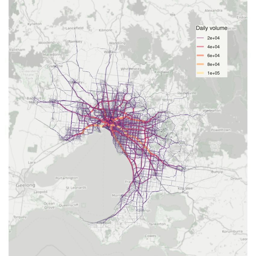
4.2 Road traffic volume analysis
Daily driving, cycling, and walking traffic volumes from the calibrated simulation out-
put are illustrated in Figure 7.
Publicly available traffic count data for Melbourne was used to examine the road
usage accuracy of the model for driving. We used the Typical Hourly Traffic Volumes
(THTV) data from Victoria’s open data platform for 2019,16 which provides the typical
traffic volumes for major arterial roads across Victoria. THTV was filtered down to the
data for school term normal mid-week days. Then the data were divided into two
categories of roads: towards Melbourne CBD (handling most of the AM peak traffic)
and those going outward from the CBD (handling PM peak traffic). In each category
(i.e., AM and PM), the top 10% highest traffic roads were identified, and within each,
the road segment with the maximum volume was selected for comparison with the
simulation output. This resulted in 87 road segments, 47 for AM peak and 40 for PM
peak hours, being selected for further analysis.
The selected road segments were joined to their equivalent links in the simulation
road network. For this purpose, the ’equivalent’ link was selected as the link located
closest to the midpoint of the road segment that satisfied the conditions of operating in
the correct direction to match the road, and having a bearing (or azimuth) within 17.5
degrees of the bearing of the road segment.
For the cycling traffic volume comparison, the average weekday daily cycling vol-
ume from automatic cycling volume and speed sensors for Greater Melbourne was
16 https://data.vicroads.vic.gov.au/Metadata/Typical%20Hourly%
20Traffic%20Volumes.html, accessed on 14/05/2021
19(a) Driving (b) Cycling
(c) Walking
Figure 7: Simulation output aggregated daily traffic volume for different modes
used, downloaded from Victoria’s open data platform for the period of March 2019.17
Each sensor was joined to its equivalent link in the simulation road network, by select-
ing the closest link that was either a bicycle path or a road with a bicycle lane and that
operated in the correct direction. In total, 48 counting sensors (some mono-directional
and others bi-directional), corresponding to 70 network links, were selected for further
analysis.
For walking traffic volume, we used pedestrian counting automated sensor data
located across Melbourne’s central LGA, i.e., City of Melbourne, encompassing the
Central Business District and surroundings (City of Melbourne, 2021). The data was
downloaded for mid-week work days of March 2019 and was joined to the simulation
road network by selecting the closest links having similar bearings to the relevant foot-
paths, in a similar way as described above for driving volumes. Given the footpaths are
17 https://discover.data.vic.gov.au/dataset/bicycle-volume-and-speed
20bi-directional, the aggregated number of pedestrians passing each sensor, regardless of
the walking direction, were used for comparison. Furthermore, for streets with more
than one footpath, the aggregated volume from all associated footpaths was used. This
resulted in selecting 48 sensors corresponding to 93 network links for further analysis.
The traffic volume percentage of the daily traffic for every hour of the day, h, and
for every road segment was calculated for the calibrated simulation output, s0h and the
observation data from THTV, sh , using Equation 6.
vr,h
sr,h = P23 , (6)
h=0 vr,h
where N is the total number of road segments analysed, and vr,h is the traffic
volume of road r during the hour h. Figure 8a depicts the average traffic volume
percentage of the daily traffic for every hour of the day across all selected N = 87 road
segments. We then used Weighted Absolute Percentage Error (WAPE) to compare the
hourly road traffic volume percentages in the observation data and simulation outputs
(Equation 7).
PN 0
r=1 |sr,h − sr,h |
W AP Eh = PN . (7)
r=1 |sr,h |
As shown in Figures 9a and 8a the simulation model does well in capturing the
peak hours car traffic volume in Melbourne with WAPE under 25%. A potential rea-
son for the car traffic volume deviations in the early morning and late evening was not
having freight traffic, travellers from outside the Greater Melbourne area and airport
passengers in the current version of the model, whose absence is likely to be more
noticeable during off-peak hours when roads are not already congested with local com-
muters. A similar trend was also observed for walking as shown in Figure 9c. For
cycling, however, the traffic volume percentage error was high throughout the day, and
considerably higher at off-peak hours (Figures 9b and 8). This was likely due to not
including the impact of cycling-relevant road infrastructure, such as bikeway type or
slope, on cycling route choice behaviour as discussed further in Section 5.
4.3 Public transport usage analysis
To validate the public transport usage in the model, the real-world percentage of pas-
senger flow aggregated at LGA level was compared with the outputs of our simula-
tion. To calculate this percentage, the passenger flow of 218 train stations across the
Greater Melbourne Metropolitan area was aggregated based on the LGA they were lo-
cated within. Then, the aggregated share of the passenger flow of each LGA relative
to the total passengers of Greater Melbourne was calculated for further comparison.
Station Access survey data from Public Transport Victoria for 2016 was used for this
comparison. This data was obtained from Victoria’s Department of Transport – Public
21(a) Driving (b) Cycling
(c) Walking
Figure 8: Aggregated hourly traffic volume percentages in simulation versus observa-
tion for different travel modes.
Transport Victoria. Figure 10 shows the comparison of real-world observations and
our simulation outputs, indicating that the simulation model was able to capture the PT
passenger flow distribution across the Greater Melbourne.
4.4 Travel distance and time analysis
Mode share and road traffic volume analyses evaluated the model at an aggregated
level, i.e., either aggregated to the travel modes or road segments. We conducted an-
other analysis on travel distance and time of a sample of trips to also evaluate the model
at the individual trip level. To do this, a subset of 1,000 trips, stratified by the origin
SA3 and travel mode, were randomly sampled from the simulated trips. Experienced
travel distance and time for the sample trips were extracted from the simulation output.
The simulated travel time for driving incorporated the impact of road congestion in
addition to speed limits and the vehicle’s maximum speed. This is due to the MATSim
queue model for capturing road traffic for the travel modes being set to use the road
network. Walking and cycling were also network modes, however, they were set not
to impact or be impacted by the road traffic, hence their travel time and distance were
simplified reflective of the network distance between origin and destination and their
constant speeds, 1.7m/s for walking and 5.5m/s for cycling. PT travel time was based
on the transit schedules extracted from GTFS and the agent’s decision about which PT
service to use.
22(a) Driving (b) Cycling
(c) Walking
Figure 9: Weighted absolute percentage error of aggregated hourly traffic volume per-
centages in simulation versus observation for different travel modes.
We used the Google Distance API to estimate the expected travel distance and
time for the sampled trips. For driving and PT, Google Distance API estimates travel
distance and time based on its historical records, taking into consideration the traffic
and network conditions. For cycling and walking, Google only assumes the fastest
route. Another limitation of using Google Distance API is that it does not provide
estimates for a past trip. Therefore, the travel distances and time of a sample of trips
were estimated based on October 2021 Google data.
Figure 11 illustrates the percentage error of travel distance and travel time for dif-
ferent modes for the 1,000 sampled trips. For example, the percentage error of travel
distance for a sample trip j and mode m, dm,j , was calculated as follows:
d0m,j − dm,j
dm,j = 100 × , (8)
dm,j
where d0m,j is the experienced travel distance from the simulation for mode m and trip
j and dm,j is the expected travel distance from Google Distance API.
23Figure 10: Passenger flow percentage comparison at the LGA level in real-world and
simulation outputs.
5 Discussion and Conclusion
In this paper, we developed an open18 multi-modal activity-based and agent-based
model for the Greater Melbourne area. We described the complete workflow of the
model development from creating the simulation scenario inputs (i.e., road network,
synthetic population, and mode choice parameters), to mode choice model calibra-
tion and simulation output analysis. All the tools we described and developed for the
AToM model are open and publicly available in our GitHub repository. Furthermore,
these tools were designed to utilise data sources that are commonly available for differ-
ent cities around the world (e.g., travel surveys, traffic counts, OSM, and GTFS). This
means although the format of some of the data used in this paper might be specific to
Melbourne, such as VISTA or traffic counts, the same workflow could be used for other
cities if the data structure is compatible with the expected structure of each tool.
The tools we presented as part of the model development workflow, such as pop-
ulation demand,19 network supply generation,20 and mode choice model estimation21
processes, serve as standalone models in their own right. Therefore, these models are
suitable for more general use outside of MATSim.
We calibrated the mode choice behaviour of the work trips for four travel modes
18 For
the steps that closed data were used for better accuracy or due to the availability of data, we made
output estimations or rasterised information extracted from them openly available so that the complete work-
flow can be reproduced by the user community.
19 https://github.com/orgs/matsim-melbourne/demand
20 https://github.com/orgs/matsim-melbourne/network
21 https://github.com/matsim-melbourne/choice-model
24(a) Travel distance (%) (b) Travel time (%)
Figure 11: Percentage error of travel (a) distance and (b) time between simulation
output and Google Distance Matrix API estimates for sampled trips
of driving, PT, walking, and cycling against the ABS Census Method of Travel to
Work 2016 and also VISTA 2016-18 (Table 5). The simulated mode share percent-
age for non-work trips also resembled the figures observed in the travel survey. The
mode choice calibrated simulation model could be used as the baseline for examining
the potential for mode shift as a result of the built environment, infrastructure and/or
monetary interventions, such as constructing new roads or modifying an existing road,
increasing PT services to existing stations, adding new stations and service lines, or
changing PT fares or motor vehicle fuel prices.
In addition to mode choice, the car traffic volumes as well as the PT passenger
flow at the LGA level from the simulation model output also resemble the volumes
observed in the real world, Figures 8a and 10, respectively. Figure 11 shows that in ad-
dition to the road level and aggregated level, the model results also reflect the expected
behaviour in terms of travel time and distance at the trip level. The realistic road traffic
behaviour of the model makes it suitable for examining various traffic management in-
terventions such as modifying speed limits or blocking certain roads to guide the traffic
flow. For example, a snapshot of car traffic on roads within 10km radius of the Mel-
bourne CBD for 9 AM and 5 PM is illustrated in Figure 12, depicting heavy congestion
on major roads connecting the Melbourne CBD to rest of the metropolitan area. Using
agent-based models, it is possible to go beyond high-level snapshots and examine the
road usage at the individual level. For instance, one of the road segments with heavy
congestion both in AM and PM peak hours is the West Gate Bridge, Victoria’s most
heavily used bridge, which is responsible for connecting the Melbourne CBD to the
western suburbs. Figure 13a illustrates where vehicles using this road segment at 9AM
are coming from and heading to, confirming the critical role the bridge is playing in
connecting the western suburbs to rest of the centre and to east. Furthermore, the travel
25route of an example agent using this bridge at 9 AM is also highlighted in Figure 13b.
(a) Morning peak at 9 AM (b) Evening peak at 5 PM
Figure 12: Snapshots of the simulated car traffic at (a) morning peak (9:00 AM) and
(b) evening peak (5:00 PM) for inner Melbourne. Colours represent the relative speed
with red = full stop, yellow = travelling speed equal to half of the speed limit, green =
travelling speed equal to the speed limit.
(a) (b)
Figure 13: West Gate Bridge 9:00 AM snapshot of (a) where the agents using it are
coming from and travelling to and (b) simulated travel route of an example agent using
the bridge.
All categories of roads accessible to the public were included in the road network
of the model, including minor bike paths to local streets and to major arterial roads
and highways. Therefore, in addition to common measures such as zone-to–to-zone
movements or traffic on major highways and corridors, our model can be used for
exploring local road usage for accessing local destinations. Further calibration for
local road usage is needed to get reliable local road usage for active modes of transport
from the model.
Unavailability of proper data on walking and cyclists’ behaviour at the city scale
has been a major barrier in designing interventions for promoting active transport. Typ-
ically available city-scale data for walking and cycling are limited to selected counting
26You can also read