An optomechanical platform for quantum hypothesis testing for collapse models - IOPscience
←
→
Page content transcription
If your browser does not render page correctly, please read the page content below
PAPER • OPEN ACCESS

An optomechanical platform for quantum hypothesis testing for collapse
models
To cite this article: Marta Maria Marchese et al 2021 New J. Phys. 23 043022

View the article online for updates and enhancements.

                               This content was downloaded from IP address 46.4.80.155 on 08/05/2021 at 05:25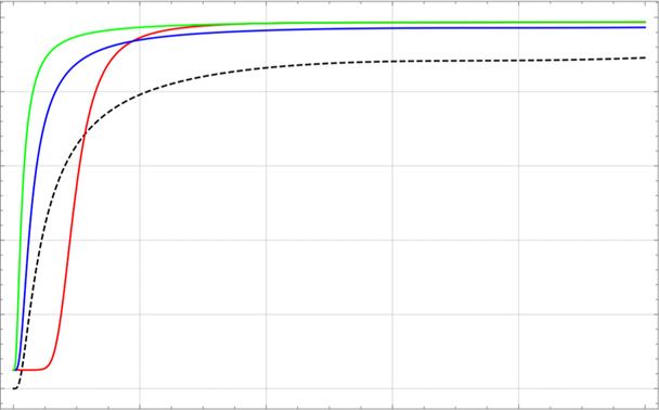
New J. Phys. 23 (2021) 043022                                                                https://doi.org/10.1088/1367-2630/abec0d

                                 PAPER

                                 An optomechanical platform for quantum hypothesis testing for
O P E N AC C E S S
                                 collapse models
R E C E IVE D
10 December 2020
                                 Marta Maria Marchese1 , ∗          , Alessio Belenchia1 , Stefano Pirandola2 and
R E VISE D
15 February 2021                 Mauro Paternostro1
                                 1
AC C E PTE D FOR PUBL IC ATION
                                     Centre for Theoretical Atomic, Molecular, and Optical Physics, School of Mathematics and Physics, Queens University, Belfast BT7
4 March 2021                         1NN, United Kingdom
                                 2
PUBL ISHE D
                                     Computer Science and York Centre for Quantum Technologies, University of York, York YO10 5GH, United Kingdom
                                 ∗
8 April 2021                         Author to whom any correspondence should be addressed.
                                 E-mail: mmarchese01@qub.ac.uk
Original content from            Keywords: quantum hypothesis testing, quantum optomechanics, collapse models
this work may be used
under the terms of the
Creative Commons
Attribution 4.0 licence.
Any further distribution
                                 Abstract
of this work must                Quantum hypothesis testing has shown the advantages that quantum resources can offer in the
maintain attribution to
the author(s) and the            discrimination of competing hypothesis. Here, we apply this framework to optomechanical
title of the work, journal       systems and fundamental physics questions. In particular, we focus on an optomechanical system
citation and DOI.
                                 composed of two cavities employed to perform quantum channel discrimination. We show that
                                 input squeezed optical noise, and feasible measurement schemes on the output cavity modes, allow
                                 to obtain an advantage with respect to any comparable classical schemes. We apply these results to
                                 the discrimination of models of spontaneous collapse of the wavefunction, highlighting the
                                 possibilities offered by this scheme for fundamental physics searches.

                                 1. Introduction

                                 Hypothesis testing (HT) is an hallmark of any statistical inference toolkit, allowing to discern between the
                                 outcomes resulting from the occurrence (or lack thereof) of unknown stochastic processes whose events
                                 occur with a set of a priori probabilities. Quantum hypothesis testing (QHT), initially introduced for state
                                 discrimination tasks [1–4], has been applied to channel discrimination and dynamics and its technological
                                 potentials in fields like quantum sensing and data read-out are under active investigation [5–9]. The
                                 characteristic of QHT protocols is that they allow to gain an advantage, in terms of lower error probabilities
                                 and in certain parameters range, over any classical HT strategy by exploiting quantum resources (like
                                 entangled squeezed light).
                                     With the advent of the second quantum revolution, quantum technologies manipulating individual
                                 quantum systems and employing exquisitely quantum resources to perform tasks are becoming a reality.
                                 Crucially, this has also renewed the interest for fundamental investigations of some of the foundational
                                 puzzles of quantum theory. Among them, the quantum-to-classical (QtC) transition—i.e., the process
                                 through which the classical world we experience in our daily life emerges from quantum mechanical
                                 building blocks [10]—plays a prominent role. Indeed, getting a grasp of the mechanisms governing the QtC
                                 could potentially settle some of the interpretational hurdles of quantum mechanics and possibly determine
                                 the ultimate limits of validity (if any) of quantum theory itself.
                                     Collapse models (CMs) [11] are one of the most prominent attempts at modifying quantum theory by
                                 promoting the collapse of the wavefunction to a physical process embedded in the laws of dynamics by a
                                 stochastic modification of the Schrödinger equation. In these models, microscopic systems evolves
                                 essentially undisturbed by the stochastic collapse, recovering all the predictions of quantum mechanics,
                                 while macroscopic objects are subject to a strong localization in position space essentially ruling out
                                 Schrödinger’s cat-like superpositions. One of the most studied CMs is the so called continuous spontaneous
                                 localization model (CSL) [12], whose phenomenology has received considerable attention in the last few
                                 years [11, 13–17]. In light of this fact, and due to the simplicity of the model, in this work we will focus on

                                 © 2021 The Author(s). Published by IOP Publishing Ltd on behalf of the Institute of Physics and Deutsche Physikalische Gesellschaft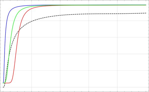
New J. Phys. 23 (2021) 043022                                                                       M M Marchese et al

CSL. It is important to note that, while CSL postulates a stochastic modification of the Schrödinger
equation, at the phenomenological level the effect of the model is captured entirely by a dissipative term
appearing in the master equation describing close quantum systems dynamics. It is thus clear that, in
realistic situations the omnipresence of the environment, and thus the open character of the dynamics,
requires sophisticated estimation and inference techniques to discriminate the presence or lack thereof of
the CSL mechanism.
    Since CMs recover all the predictions of quantum mechanics for microscopic systems, it is clear that
tests able to constrain the parameter space of such models should employ mesoscopic quantum systems.
However, creating large spatial superposition of mesoscopic objects is inherently challenging and the subject
of intense investigation [18–21]. Fortunately, CMs can also be probed via non-interferometric techniques
[22–26] which do not require the creation and verification of large superpositions. This is exactly the case
we explore in this work where the CSL affect the mesoscopic mechanical oscillator in an optomechanical
set-up. It is well known that in this situation, the effect of the CSL can be interpreted as an extra mechanical
dumping source or, alternatively, as an increased equilibrium temperature of the oscillator. Owing to this,
several non-interferometric tests of CMs have been proposed, and experiments have been carried out
constraining the parameter space of the CSL model (cf reference [11] and references therein). Inference
techniques translated from quantum metrology and estimation theory have been widely employed in such
endeavours. Recently, HT has been embedded in theoretical schemes for the assessment of macrorealism
and collapse mechanisms [27, 28]. In this work, we consider HT for channel discrimination to probe the
dynamical effects of CMs on macroscopic mechanical oscillators.
    We thus face the challenge of discriminating between two quantum channels, encoding the presence or
lack of CSL, characterizing the dynamics of the mechanical mode. QHT is particularly apt to this task and
we set to show that quantum resources can be used to overcome any comparable classical strategy.
Furthermore, we propose in the following a specific measurement strategy to perform the HT based on
realistic parameters for the optomechanical systems. In this way, we do not aim to establish the ultimate
advantages that a QHT strategy can allow—which could result in a hardly feasible measurement
scheme—but we explicitly spell out one strategy that is both feasible within current technology and that
presents the aforementioned quantum advantage.
    The remainder of this work is organized as follow. In section 2 we introduce the optomechanical set-up
of interest and we spell out the effect of the CSL on the dynamics of the mechanical mode. In section 3 we
lay down the measurement schemes that we are going to consider in our analysis. Section 4 summarises the
main concepts of HT and introduces the classical bound we are going to compare the quantum case with.
Section 5 presents the main results of our work. Finally, we concluded in section 6 with a discussion of our
findings.

2. The system

Let us consider a system composed by two optical cavities of length L, as shown in figure 1. We follow here
the discussion in reference [29] where a similar optomechanical system was investigated for entanglement
distribution. Note however that here we make use of a single mechanical oscillator, as a second one would
not result in a better performance of the scheme proposed in this work. The cavity modes with frequency
ω C are described by creation and annihilation operators {â†i , âi }, with i = 1, 2. The first cavity is equipped
with a movable mirror characterised by position and momentum operators {q̂, p̂} and damping rate γ m .
The second cavity is a simple Fabry–Perot cavity with energy decay rate κ, identical to the first one. They
are initially pumped with coherent light with frequency ωL and power P. The Hamiltonian describing the
system reads as
                                                           p̂2     mωm  2

                      Ĥ =       δâ†i âi + i â†i − âi +         +        q̂2 − χâ†1 â1 q̂,              (1)
                           i=1,2
                                                                2m         2

where δ = ω C − ω L is the cavity-pump detuning, ω m is the frequency of the mechanical oscillator,
χ = ω C /L is the radiation-pressure coupling constant and  = 2kP/ωC is the amplitude of the laser field
which we treat as classical from now on.
    When the pumping field is intense enough, as we assume in the following, the description of the
dynamics simplifies enormously since we can linearize both the cavity and mechanical modes around their
respective steady-state. We thus consider the dynamics of the sole zero-mean quadratures fluctuations that
we order in the vector
                                         r̂ = Q̂, P̂, X̂ 1 , Ŷ 1 , X̂ 2 , Ŷ 2 .                       (2)
Here, the first two elements are the dimensionless quadratures for the mechanical mode

                                               2
New J. Phys. 23 (2021) 043022 M M Marchese et al
Figure 1. Two cavities, one embedded with a movable mirror, are pumped with a classical laser field (red-shaded region) and
with an extra source made of two modes of light (green line). Input modes go through polarizing beam splitters, enter the
cavities, interacting with them and, when they come out, they pass through a quarter-wave plates, which will change the
polarization and will allow us to collect the output modes. Before performing the measurement, we might recombine the outputs
using a beam splitter. The two-cavity set-up is crucial for harnessing the quantum advantage entailed by the use of two-mode
squeezed light in a ‘quantum reading’ like scheme.
mωm 1
Q̂ = q̂, P̂ = √ p̂ (3)
mωm
with Q̂, P̂ = i. The remaining components of the vector represent the optical quadratures
â†j + âj â†j − âj
X̂ j = √ , Ŷ j = i √ (with i = 1, 2), (4)
2 2
for the two intra-cavity field modes.
The quadrature vector evolves in time according to the Langevin equations in the input–output
formalism
r̂˙ = Ar̂ + n̂. (5)
where the 6 × 6 drift matrix A is given by
⎛ ⎞
0 ωm √0 0 0 0
⎜ −ωm −γm 2αg 0 0 0 ⎟
⎜ ⎟
⎜ 0 0 −κ δ 0 0 ⎟
A=⎜ √
⎜ 2αg
⎟ (6)
⎜ 0 −δ −κ 0 0 ⎟
⎟
⎝ 0 0 0 0 −κ δ ⎠
0 0 0 0 −δ −κ
with α = R[a] the square root of the number of photons in the cavity and g = χ /mωm the effective
coupling rate. The vector n̂ collects the zero-mean quantum noise operators and it is given by
√ √ √ √
n̂ = 0, ξ̂, 2κX̂ in1 , 2κŶ in1 , 2κX̂ in2 , 2κŶ in2 . (7)
Here, ξ̂ is a Langevin force operator encoding the interaction of the mechanical mode with a phononic
thermal bath at temperature T and producing the Brownian motion of the mechanical oscillator. This noise
is characterised by its two-point correlator which can be written as
2γm kB T
ξ(t)ξ(t ) = δ(t − t ), (8)
ωm
in the high temperature limit kB T ω [30]. Then X̂ ink , Ŷ ink , with k = {1, 2}, are the quadratures of the
input noises impinging on the two cavities. The covariance matrix of these two input modes encodes the
information on the light state we feed to the cavities on top of the coherent pumping.
In the linearized picture that we are considering, the total Hamiltonian of the system is at most
quadratic in the quadratures r̂ while the Lindblad operators, describing the interaction with the phononic
3New J. Phys. 23 (2021) 043022 M M Marchese et al
thermal bath, are at most linear in them. Thus, if both the initial state of the modes r̂ and the state of the
input noises are Gaussian, the dynamics will preserve this Gaussianity [31, 32]. This observation
enormously simplify the dynamics of the system since it is enough to consider the evolution of the first and
second statistical moments of the quadratures of the system. Furthermore, as we consider zero-mean
quantum fluctuations and the dynamics of the mean values is decoupled from the evolution of the
variances, it is sufficient to work with the time evolution of the covariance matrix σ, which is ruled by the
Lyapunov-like equation
σ̇ = Aσ + σAT + D, (9)
where D is the so-called diffusion matrix. The elements of D depend on the two-point correlations of the
noise vector as [33]
1
Dij = ni (t)nj (t) + nj (t)ni (t) . (10)
2
Considering the aforementioned sources of noise, we can express the 6 × 6 diffusion matrix D in
block-diagonal form as
σm 0
D= , (11)
0 σ IN
where σ IN is the 4 × 4 dimensionless covariance matrix associated to the input modes times 2κ, while
⎛ ⎞
0 0
σm = ⎝ γm kB T ⎠ (12)
0 2 +Δ
ωm
is the 2 × 2 matrix describing the thermal dissipation.
Note that, in the last term entering the diffusion matrix we have introduced an extra heating rate
parameter Δ. This parameter de facto modifies the equilibrium temperature of the mechanical oscillator
and correspond to an extra dissipation channel for the open quantum system composed by the two cavity
modes and the mechanical one. Before moving on, let us briefly remark in the following that the stochastic
effect of the CSL model on the mechanical mode in cavity one is encoded exactly in the extra parameter Δ
appearing in the diffusion matrix.
2.1. Continuous spontaneous localization model
CMs [11] introduce stochastic modifications to the Schrödinger equation of quantum mechanics in the
attempt to promote the collapse of the wavefunction to a dynamical process providing a dynamical picture
of how the classical world emerges from the quantum microscopic one. For our purposes here we do not
need to go into the details of CMs. It is enough to say that we will make use of the arguably better studied
among CMs, the so called CSL model.
The CSL, with white noise, describes the collapse as a continuous process in time. This introduces in the
master equation of the system an extra spatial decoherence term whose phenomenology is completely
characterized by two parameters {rC , γ}. The parameter rC , is the localization length of the model, i.e., the
characteristic length-scale above which the collapse mechanism is relevant. The collapse rate γ sets the
strength of the CSL mechanism [11].
In our setting, the CSL mechanism affects in a significant way only the mechanical mode due to its
‘mesoscopic nature’ in view of the fact that CMs are formulated in such a way that their predictions deviate
from standard quantum mechanics only for meso-/macroscopic systems. Our mechanical mode is in
contact with a thermal phonon bath at temperature T, whose effect is described by the operator ξ̂ in
equation (7). On top of that, we consider the decoherence induced by the CSL. Formally, we can treat the
effect of the CSL by defining a modified equilibrium temperature of the oscillator via
Δ
γm (2n̄th + 1) + Δ = Δ(2nCSL + 1) → nCSL = n̄th + . (13)
2γm
where n̄th is the thermal number of phonons at temperature T. The parameter Δ entering this expression
and the diffusion matrix in (12) is a function of both rC and γ as well as the mass distribution of the system
of interest. As reported in [34] it can be written explicitly as
|r−r |2
−
3 2
γ e 4rC
Δ= √ ∂r ρ(r)∂r ρ(r )dr dr , (14)
3mωm m20 (2 πrC )3 k k
k =1
where m0 = 1 amu (atomic mass unit) and ρ(r) is the mass density of the system subject to the CSL.
4New J. Phys. 23 (2021) 043022 M M Marchese et al
Figure 2. On the left a scheme for the measurement of EPR quadratures, while on the right for a local measurement. The scheme
in figure 1, captures the case on the left here, i.e., EPR quadratures measurement. In order to implement the classical scheme on
the right, it would be sufficient to remove the beam-splitter in figure 1 combining the output cavity modes.
3. Measurement schemes
The main objective of this work is to investigate the potential of optomechanical systems and quantum
reading protocols [35, 36] for the discrimination of the additional dissipative channel described by the
parameter Δ via the methods of QHT. In particular, we want to determine whether quantum resources, in
the form of non-classical input noise states, can lead to a quantum advantage with respect to classical
resources for HT. In order to accomplish this, we will examine two cases for the state of the input noise
modes: (i) a two-mode squeezed state (TMS) as an entangled, and thus quantum, resource and (ii) two
independent thermal states as classical ones.
Furthermore, in order to probe the system the output modes emerging from the two cavities needs to be
measured. Also at this stage we can consider different measurement strategies with different ‘degrees of
quantumness’ at play, see figure 2. The output modes can be directed towards photodetectors by using a
combination of quarter waveplates and polarised beamsplitters (see figure 1). We then consider two
different measurement schemes: (i) a local measurement, consisting in measuring directly the quadratures
of the output modes {x̂outi , ŷouti } with i = 1, 2; (ii) in the spirit of the original quantum reading protocol
[35], the output modes can be further recombined through another beamsplitter to perform a
measurements of Einstein-Podolsky-Rosen (EPR)-like quadratures {q̂∓ , p̂± } of the emerging modes {+, −}.
These are defined as ⎧
⎪ x̂out1 ∓ x̂out2
⎨q̂∓ = √
2 (15)
⎪ ŷout1 ± ŷout2
⎩p̂± = √ ,
2
in term of the output modes.
Finally note that, using the input–output formalism [37], the output modes can be easily expressed in
terms of the input ones via ⎧
⎨x̂ √
out1,2 = κX̂ 1,2 − X̂ in1,2
√
⎩ŷout = κŶ 1,2 − Ŷ in .
(16)
1,2 1,2
All the output modes will depend on the parameter Δ, which vanishes in the case where no CSL is present.
For simplicity of notation we omit the dependence on this parameter. It should also be noticed that, such
dependence arises owing to the dynamics of the mechanical system. By itself, the CSL mechanism does not
influence light and this guarantee the read-out of the CSL effect on the mechanical oscillator in our set-up.
3.1. Initial state
While not strictly part of the measurement strategy, we comment here on the initial state of the system
(cavities + mechanical mode) that we will assume in the rest of the work unless otherwise stated. Indeed,
the choice of a particular initial state is undoubtedly part of any protocol and one on which the feasibility of
the protocol hinge.
In view of these considerations, we consider as initial state the product state of the cavities’ steady-states
when subject to vacuum input noises (i.e., when only the coherent pumping is present). The result is a state
in which the mechanical mode and the first cavity reach their joint steady-state, fully characterized by the
covariance matrix σ mcss , while the optical mode of the second cavity remains in its ground state
(17)
where In×m and On×m are n × m identity and zeros matrices, respectively. This choice of initial state
corresponds in practice to commencing the experiment without additional light sources and wait long
5New J. Phys. 23 (2021) 043022 M M Marchese et al
enough for the system to reach its steady-state. After this, we can start to probe the cavities with extra
modes of light (the input noises) and measure the output cavity fields as described above.
3.2. Protocol description
Before proceeding further and introducing the HT, let us summarize the steps of our channel
discrimination protocol:
(a) Preparation: the optomechanical system, subject to only the coherent pumping of the cavities (i.e.,
vacuum input noise) reaches its steady-state;
(b) Classical/quantum resources: two additional light mode impinge on the cavity and are prepared in
either a TMS state or in the tensor product of two local thermal states. The system starts to evolve away
from the initial state;
(c) Measurements: at the same time as the input noises are fed into the cavity, we can monitor the output
modes via photodetectors. This can be perform either via local measurement or measuring EPR-like
quadratures after recombining the output modes via a beamsplitter;
(d) Post-processing: the obtained measurement outputs are post-processed via a χ2 -test to discriminate
the possible channels, i.e. if the parameter Δ vanishes or not.
While we will discuss in detail the HT post-processing in the next section, it should be noted that the
χ2 -test is suitable since the output of the quadratures measurements follow a Gaussian distribution with
zero-mean and variance depending on Δ.
4. Quantum hypothesis testing
In this section, we summarize the main elements of HT and specify the classical bound to the error
probability in our specific set-up. This lays the basis for comparison between classical and quantum
protocols and to show an advantage in using quantum resources.
In a typical binary HT, two exclusive hypotheses are formulated. Hypothesis H0 is called null hypothesis
and it is the starting point: we assume this to be true and we will conduct a test to determine whether this is
likely to hold or not. The alternative hypothesis H1 contradicts the previous one and expresses what we
think is wrong in the null hypothesis. In our set-up, we aim at testing whether the dissipative channel
associated to Δ is present. This also means testing if the effect coming from CSL model is present or not. In
this context, H0 corresponds to no new physics, i.e. an open dynamics with no CSL, while H1 to the
presence of the extra dissipative mechanism.
The HT is performed by post-processing the measurement outcomes. As highlighted in the previous
section, these outcomes follow zero-mean Gaussian distributions. This implies that the HT, and so the
channel discrimination, corresponding to discriminating two Gaussians with different variances (V0 , V1 )
depending on Δ. Thus we can formulate the two hypotheses as follow
⎧
⎨H : Δ = 0 ⇐⇒ V = V
0 0
(18)
⎩H1 : Δ > 0 ⇐⇒ V = V1 = V0 .
Moreover, it is easy to verify that, for Δ > 0 the condition V1 > V0 holds for both the outcomes of local
measurement of the output variables and EPR-like variables. This implies that we can conduct a one-tail
test.
It is important to note that, in general, Δ 0, with Δ = 0 corresponding to the absence of the CSL.
Therefore, statistical inference methods can only rule out, with a certain likelihood, some parts of the CSL
parameter space casting upper bounds on rC and γ.
Given the nature of the problem, we use a χ2 -test in the following by defining the test statistic
T = (N − 1)s2 /V0 , where s2 = N i=1 (ri − r̄ i ) /N − 1 is the sample variance for a sample-size N, and ri is
2
the variable we decide to use for the test among {q± , p∓ }, for EPR-like measurements, or {xout1,2 , yout1,2 } for
the classical ones. The test statistic follows a χ2 -distribution with N − 1 degrees of freedom. Note that,
contrary to the quantum reading protocol in [35], in our case for each measurement schemes different
quadratures have different variances. This means that they should be subjected to separate tests not allowing
to double the number of outcomes as in [35].
In an experiment, the HT proceed by comparing the likelihood for the particular realization of the test
statistic T = t∗ with the so called significance level α of the test, i.e. the maximum error that we allow
ourselves to commit by rejecting H0 when true. In particular,
6New J. Phys. 23 (2021) 043022 M M Marchese et al
⎧
⎨if t ∗ QN−1 ⇐⇒ P| (T t ∗ ) α ⇒ reject H
1−α H0 0
(19)
⎩if t ∗ < QN−1 ⇐⇒ P|H (T t ∗ ) > α ⇒ accept H0 .
1−α 0
Here we indicate with P|H0 (T t ∗ ) the probability of obtaining a value of the random variable T larger
then t∗ conditioned on assuming H0 is true. Note that, as usual, the condition on the probability are
mirrored by condition on the realization of the statistic in terms of the quantiles of the χ2 -distribution
QN−1
1−α .
Crucial quantities in HT are the error probabilities, i.e. the probability of rejecting H0 when true and the
probability of accepting H0 when false. The former is known as type I error and quantified by P(H1 |H0 ), the
latter is a type II error quantified
by P(H0 |H1 ). Assuming
error priors for the two hypotheses, the mean
error probability is Perr = P(H1 |H0 ) + P(H0 |H1 ) /2. It is a simple exercise to find the expression for the
total error probability given by
⎡ ⎤
N−1 N−1
N−1 Q1−α V0 N−1 Q1−α
1⎢
Γ 2 , 2V1 Γ 2 , 2 ⎥
Perr = ⎢ ⎣ 1 − N−1
+ N−1
⎥,
⎦ (20)
2 Γ 2 Γ 2
where Γ(z, x) and Γ(z) are the incomplete and complete Gamma functions, respectively.
Finally, while the values of V0,1 entering the error probability expression depend on both the initial noise
state and the measurement scheme, their functional form depends only on the latter. In particular, using the
input–output relations and the ordering of the system degrees of freedom for the elements of covariance
matrix of the system σ(t) as in equation (2) it is easy to obtain the expressions for the variances of the
output results. For example we have
Var(xout,1 ) = 2κσ33 (21)
Var(q± ) = κ (σ33 + σ55 ± 2σ35 ) , (22)
where σ ij are the elements of the covariance matrix solving equation (9),and analogously for the rest of the
measured quadratures. The dependence of these expressions on the initial noises, as well as on the unknown
parameter Δ, is hidden in the elements of the covariance matrix σ(t) coming from solving the dynamics.
We identify V0,1 in the HT with the values of the relevant variances—depending on the measurement
scheme and initial noise chosen—for Δ = 0 or Δ > 0 respectively.
4.1. Classical bound
We now show that, at intermediate times, quantum resources allow to attain a total error probability lower
than the one achievable by any comparable classical strategy. In order to claim this, we need a measure of
the minimum error probability attainable. Following the results in theorem 4 of [35] for the discrimination
of two Gaussian channel via a classical protocol, the error probability is lower-bounded by
√
1 − 1 − (F(n1 , n2 , t))N
C(n1 , n2 , t) := , (23)
2
where F(n1 , n2 , t) is the fidelity between the two-mode output Gaussian states corresponding to the
evolution of the system up to time t when Δ = 0 or Δ > 0 with classical input noise thermal states
characterized by n1 and n2 mean photon numbers [38].3 N is again the number of measurement outcomes
collected at time t.
Equation (23) is the most stringent bound to the error probability to discriminate the two Gaussian
states ρΛ=0 and ρΛ=0 [38]. It is obtained from the form for the error probability derived by Helstrom [1],
Perr (ρ0 , ρ1 ) =√1 − D(ρ0 , ρ1 ) where D(ρ0 , ρ1 ) is the trace distance, by using the inequality
D(ρ0 , ρ1 ) 1# − F(ρ0 , ρ1 ) and the factorization properties of the quantum fidelity for product
states—ρ(t) = N k=1 ρk (t), with ρk the two-mode Gaussian state in each run of the experiment at time t.
5. Results
We aim to show that, the total error probability for the channel discrimination in our set-up, when the
input noises are quantum correlated, can be lower than the one that can be achieved by any comparable
classical strategy. It should be stressed that we do not aim to find the ultimate quantum bound to the error
3 It should be noted that, what we call here fidelity (F) corresponds to the fidelity squared (F 2 ) in [38].
7New J. Phys. 23 (2021) 043022 M M Marchese et al
Table 1. Specifics of all the parameters for the set-up of two cavities
and a mechanical mode entering the simulations in this work.
Symbol Name Value or expression
γm Mechanical dumping 2πω m /105
ω m /2π Mechanical frequency 2.75 × 10⁵ Hz
T Phononic bath’s temperature 10−3 K
ω C /2π Cavity mode’s frequency 9.4 × 10⁵ c
m Mass 150 ng
L Cavity length 25 mm
κ Cavities linewidth 5 × 10⁷ Hz
δ Cavity-pump detuning 4κ
P Pump laser power 4 × 10⁻³ W
R Mechanical system linear dimension 1 μm
probability. Indeed, our scope is more practical: we want to show that such an advantage exists for the
specific protocol we consider.
In what follows we fix the significance level to be α = 5% unless otherwise stated. All the values of the
system parameters used in the simulations are reported in table 1. These values are within reach of current
technology which is in favour of the feasibility of the protocol. Finally, we assume Δ = 106 Hz unless
otherwise specified. This value of the parameter, characterizing the unknown extra-channel whose presence
we want to discriminate, is such that the extra diffusion associated with it is greater than the thermal
diffusion characterized by 2γ m kB T/(ωm ) and it is motivated by the CSL model. As we discussed
previously, the CSL model with white-noise is completely characterised by the two parameters rC , and γ.
The first, rC can be fixed at 100 nm [22] while for the second one we consider the value proposed by Adler
[39] γ A = 10−28 m3 Hz. Indeed, assuming the mechanical mode to describe the center of mass of a system
with linear dimension R, that we approximate as spherical for simplicity, and using equation (14), this
choice of CSL parameters results in Δ ≈ 106 Hz.
We perform a dynamical analysis, starting from the steady-state of our three-partite system when
vacuum input noises are present, and focus on the transient before the system reaches a new steady-state. In
doing this, we compare two protocols: a classical one using input thermal noises and local measurements
of the output modes, and a quantum one with two-mode squeezed input noises and EPR-like
measurements.
In order to show the advantage coming from using quantum resources in our context, we need to
compare the quantum scheme with the classical lower bound to the error probability. A fair comparison can
be achieved by fixing the photon number in the input noises to the two cavities {n1 , n2 } and comparing
situations with the same sample size N, i.e., repetitions of the experiment. We thus compare the error
probability coming from the quantum protocol using a TMS input noise with the lower bound that can be
achieved starting from uncorrelated thermal noises with the same mean photon number per input mode as
the TMS. The lower bound, as already discussed, is the minimum error probability that can be achieved by
any classical measurement procedure [40]. Thus, the comparison with it can show possible quantum
advantages.
We start by showing the discrepancy between the local measurement strategy, with classical input
noises—a.k.a. the classical protocol—with the lower bound to the error probability C. The classical input
noise is characterized by its thermal covariance matrix
(24)
entering equation (11). Figure 3 shows the classical error probability and the correspondent bound for two
values of n1 . The value of n2 does not have any bearing on these probabilities. We can see that the classical
error probability is always greater than the classical bound, as expected, and the bigger the number of
photons we inject as noise in the first cavity the worse our ability to discriminate the two hypotheses
become.
In figure 4, we show a first comparison of the quantum error probability with respect to the classical
bound. In this case, the input noise state is a TMS state with same mean photon number on the two modes
and characterised by the squeezing parameter r 0 and the squeezing angle φ. The input covariance matrix
entering in equation (11) is given by
(25)
8New J. Phys. 23 (2021) 043022 M M Marchese et al
Figure 3. Comparison between the classical error probabilities (solid lines) and the respective bounds C (dashed lines) for
different values of the mean number of photons in the input noise’s modes, n1 = n2 . The red curves represent n1 = 10 while the
blue ones n1 = 100 and we consider the statistics of measurements for the xout1 output quadrature. As discussed in the main text,
Δ = 106 Hz which corresponds to CSL with Adler parameters [39]. The level of significance and the number of experiments are
α = 5% and N = 100 respectively.
Figure 4. Quantum error probabilities (solid lines) for different squeezing angles φ = {π/2, 5π/6, π}. The parameters are
n1 = n2 = 100, N = 100, Δ = 106 Hz, and α = 5%, and we consider the statistic of measurements for the q+ output
quadrature. The dashed curve represents the corresponding classical bound C(n1 , n2 , t), the blue curve is the quantum error
probability when the squeezing angle is φ = π/2, the green one for φ = 5π/6 and the red one corresponds to φ = π. We observe
that, for the squeezing angle approaching φ = π, violations of the classical bound are possible at intermediate times.
where
cos φ sin φ
Rφ = . (26)
sin φ − cos φ
Fixing the mean photon numbers in the two input modes corresponds to fixing the value of the squeezing
parameter r given the relation cosh 2r = 2n1,2 + 1. We are thus left with the single free parameter φ, the
squeezing angle. From figure 4, we see that, for non-vanishing squeezing angles, and looking at the statistics
of the q+ EPR quadrature, a quantum advantage appears since the error probability curve can be lower than
the corresponding classical bound. This is the main result of this work. In particular, we see that the
advantage is maximized for a squeezing angle φ = π and can be shown to be monotonically increasing for
φ ∈ (0, π]. Figure 5 shows that no advantage is obtained when we set φ = 0, for measurements of the q+
quadrature, and it also shows the dependence of the quantum error probability on the mean number of
photons in the noise input. As it could be expected, by increasing the mean number of photons in the input
noise the quantum error probability increases. In the same way, the error probability increases when
decreasing the number of repetitions of the experiment N as it is clearly shown in figure 6.
9New J. Phys. 23 (2021) 043022 M M Marchese et al
Figure 5. Comparison between quantum error probabilities (solid lines) and the corresponding classical bounds (dashed lines)
for vanishing squeezing angle, φ = 0. The blue curves are computed for n1 = n2 = 10 while the red ones for n1 = n2 = 100. In
both cases N = 100, Δ = 106 Hz, and α = 5%, and we consider the statistic of measurements for the q+ output quadrature.
Figure 6. Quantum error probabilities for φ = π (solid lines) and corresponding classical bounds (dashed lines) for varying
number of repetitions of the experiment N = 10, 100. The blue curve corresponds to N = 10, the red one to N = 100. We fix
α = 5%, Δ = 106 Hz, and n1 = n2 = 100. We consider the statistic of measurements for the q+ output quadrature.
For the sake of completeness, we examined also two additional cases: one is the combination of TMS
light and local measurements and the other is the opposite case of classical thermal input noises and EPR
measurements. Figures 7 and 8 show both these cases respectively. It is apparent that, when compared to
their respective classical bounds, the error probabilities do not show any advantage even when fixing φ = π
in the first case. This tells us that the quantum advantage as shown before depends on the combination of a
quantum input and a quantum measurement strategy. Figure 9 shows the comparison between these last
two protocols and the fully quantum one. It should be noted that, in all the previous figures, neither the
classical bounds nor the error probabilities vanish at the initial time.
When considering the error probabilities arising from the measurements of the EPR output quadratures,
in all the reported figures we have shown the statistic of the EPR quadrature q+ . This is sufficient to
demonstrate the quantum advantage by comparing error probability with the quantum bound. A similar
performance would have been obtained by considering other output quadratures. For instance, if
considering the statistics related to q− , any quantum advantage is maximized for φ = 0. This should not
come at a surprise: the occurrence of an advantage when combining TMS input noise and EPR output
measurements can be intuitively traced back to the fact that the two-modes squeezed input light allows
quantum correlations of the output fields of the two cavity, which can be exploited in an EPR measurement.
In line with the quantum reading protocol [35], such correlations appear to be a quantum resource for HT
10New J. Phys. 23 (2021) 043022 M M Marchese et al
Figure 7. Error probabilities (solid lines) for a protocol in which we have input modes in a TMS state but classical measurements
of the output modes. Here we consider local measurements of xout1 to perform the QHT. The dashed lines correspond to the
classical bounds. Parameters values are φ = π, n1 = n2 = 100, and Δ = 106 Hz. The blue curves are obtained for N = 10 and
the red ones for N = 100. This measurement scheme does not show any advantage in the form of a violation of the classical
bound.
Figure 8. Error probabilities (solid lines) for a protocol in which we have the input modes in product of thermal states and EPR
quadrature measurements for the output modes. Here we consider measurements of the quadrature q+ to perform the QHT. The
dashed lines correspond to the classical bounds. Parameters values are φ = π, n1 = n2 = 100, and Δ = 106 Hz. This
measurement scheme does not show any advantage in the form of a violation of the classical bound.
inference. In this context, the dependence of the advantage on the squeezing angle can be qualitatively
expected on the basis of the fact that—depending on the parameters of the set-up—the non-classical
correlations between the output cavity modes that can enable the advantage can be accessed by measuring
suitably rotated phase-space quadratures.
In the case of TMS input noise and local measurements, it is intuitive to understand that the quantum
correlations established between the cavities’ output modes cannot be exploited by a scheme based on local
measurements. For instance, in figures 7 and 9 no advantage is shown. Analogously, in the case of figure 8,
where classical noise is teamed with EPR measurements, no advantage is expected. Indeed, as no quantum
correlations between the output cavity modes can be present, the output mode of the second cavity is
completely oblivious to the CSL mechanism affecting the mechanical mode in the first cavity. The mixing of
the output cavity modes, entailed by the EPR measurement, can thus only additionally spoil the
discrimination process as a noise source.
Finally, the quantum advantages we have found appear at short times and in a dynamical phase away
from the steady-state. At long times we see from the previous figures that the advantage is not present
anymore. This is analogous to what happens in certain quantum metrology schemes for open quantum
11New J. Phys. 23 (2021) 043022 M M Marchese et al
Figure 9. Comparison between different protocols. 1. Red curve: TMS light as input and EPR measurements of the output
modes. 2. Blue curve: TMS light as input and classical (local) measurements of the output modes. 3. Green curve: thermal input
noises and EPR measurements. Parameters are φ = π, n1 = n2 = 100, N = 100, α = 5%, and Δ = 106 Hz. The dashed line
represents the corresponding classical bound. We consider the statistic of xout1 and q+ from the local and EPR measurements,
respectively. As already observed, the only protocol which is able to offer some advantage over the classical bound is the first, fully
quantum one.
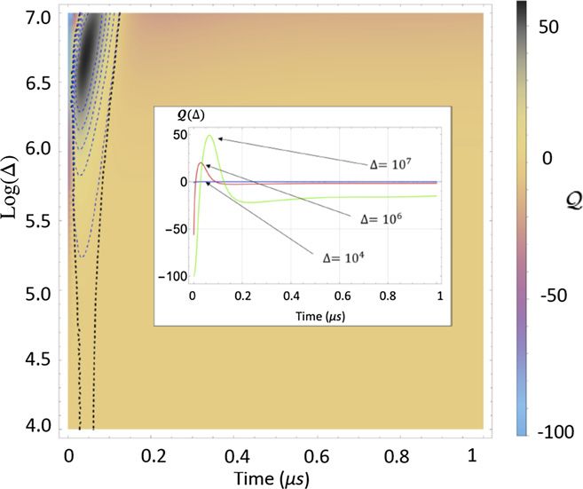
Figure 10. Quantum advantage for different values of the Δ parameter. The main figure shows a density plot of Q(Δ, t) defined
in equation (27). Parameters are n1 = n2 = 100, N = 10, α = 5% and φ = π, and we consider the statistic of measurements for
the q+ output quadrature. The black dashed contour separate the region of positive and negative Q. The blue dashed contours
are level lines in the region Q > 0, i.e., in the region in which a quantum advantage can be found. The inset shows three sample
curves for Δ = {104 , 106 , 107 } Hz in detail. It should be noted that, the case Δ = 104 Hz corresponds to the situation in which
the CSL (or the unknown heating mechanism of the mechanical mode) rate is smaller than the thermal diffusion rate. We also
observe that, for Δ = 104 Hz, despite the small quantum advantages, the quantum protocol considered delivers an error
probability close to the classical bound at any time.
systems [41] where, at long times, the effect of the dissipation is such that quantum properties are lost and
so is the advantage.
To conclude this section, and in view of the application of the QHT inference scheme presented here to
CM, it is interesting to show that the quantum advantage persists if we vary the parameter Δ. This can be
seen in figure 10, where it is shown the relative difference between the quantum error probability and the
classical bound
C(n1 , n2 , t) − Perr (φ, r, t)
Q(Δ) = 100 , (27)
C(n1 , n2 , t) + Perr (φ, r, t)
for φ = π, n1 = n2 = 100, and N = 10. This figure, and its inset, shows an advantage (regions of Q > 0)
that is present at early times and extends on several order of magnitudes of Δ. Remarkably, an advantage
12New J. Phys. 23 (2021) 043022 M M Marchese et al
can still be found also when the unknown channel effect is sub-leading with respect to the thermal diffusion
rate. An in-depth analysis of the possibilities offered by QHT for constraining CSL and related models is
outside of the scope of the present work and will be part of a future investigation.
6. Conclusions
The combination of QHT and optomechanical architectures opens the way to tests of fundamental physics
and offers the possibility of quantum advantages over analogous classical strategies.
Following an approach inspired by the quantum reading framework, we have applied QHT to
discriminate between two dynamical channels applied to an optomechanical system. Two hypotheses were
formulated to describe the absence (H0 ) or presence (H1 ) of an additional dissipative mechanism,
potentially due to the spontaneous localization of the wavefunction of the mechanical resonator as
predicted by the CSL model.
We compared two measurement strategies and we studied the associated error probabilities to infer that
there is an advantage when we use non-classical input noise states instead of classical resources.
The classical scheme uses as input source two independent thermal states and it is combined with a
direct measurement of the output modes. The quantum scheme employs a TMS state and an EPR-like
measurement. We have compared the error probabilities obtained from such schemes and the classical lower
bound that can be obtained from the fidelity of the two-mode output state with classical thermal input
noises. While the error probabilities coming from the classical protocol are always greater than the classical
bound, the same is not true for the quantum protocol error probability, which shows an advantage at finite
times for some values of the squeezing angle. Recently, in [42] it was shown how squeezing entanglement
offers an advantage for testing the CSL model in cold atom interferometric experiments. Moreover, we
explored a large part of the parameter space of the CSL mechanism, showing that the advantage is
widespread.
In the framework of CMs, this study offers a starting point to future analysis aimed to restrict the range
of still untested parameters characterizing CMs. More in general, we have proposed a versatile scheme that
could be implemented and applied to different systems in view of exploring other fundamental physics
mechanisms.
Acknowledgments
MMM and MP acknowledge support from the EU H2020 FET Project TEQ (Grant No. 766900). AB
acknowledges the MSCA project pERFEcTO (Grant No. 795782). SP acknowledges funding from the
European Union’s Horizon 2020 Research and Innovation Action under Grant Agreement No. 862644
(FET-OPEN project: Quantum readout techniques and technologies, QUARTET). MP is supported by the
DfE-SFI Investigator Programme (Grant 15/IA/2864), the Royal Society Wolfson Research Fellowship
(RSWF\R3\183013), the Royal Society International Exchanges Programme (IEC\R2\192220), the
Leverhulme Trust Research Project Grant (Grant No. RGP-2018-266), and the UK EPSRC (Grant No.
EP/T028106/1). This research was partially supported by COST Action CA15220 ‘Quantum Technologies in
Space’.
Data availability statement
All data that support the findings of this study are included within the article (and any supplementary files).
ORCID iDs
Marta Maria Marchese https://orcid.org/0000-0001-5815-1547
Alessio Belenchia https://orcid.org/0000-0002-0347-6763
Stefano Pirandola https://orcid.org/0000-0001-6165-5615
Mauro Paternostro https://orcid.org/0000-0001-8870-9134
References
[1] Helstrom C W 1976 Quantum Detection and Estimation Theory vol 3 (New York: Academic)
[2] Chefles A 2000 Contemp. Phys. 41 401
13New J. Phys. 23 (2021) 043022 M M Marchese et al
[3] Barnett S M and Croke S 2009 Adv. Opt. Photon. 1 238
[4] Weedbrook C, Pirandola S, García-Patrón R, Cerf N J, Ralph T C, Shapiro J H and Lloyd S 2012 Rev. Mod. Phys. 84 621
[5] Ortolano G, Losero E, Pirandola S, Genovese M and Ruo-Berchera I 2021 Sci. Adv. 7 eabc7796
[6] Spedalieri G, Piersimoni L, Laurino O, Braunstein S L and Pirandola S 2020 Phys. Rev. Res. 2 043260
[7] Harney C, Banchi L and Pirandola S 2020 arXiv:2010.10855 [quant-ph]
[8] Banchi L, Zhuang Q and Pirandola S 2020 arXiv:2010.03594 [quant-ph]
[9] Barzanjeh S, Pirandola S, Vitali D and Fink J M 2020 Sci. Adv. 6 eabb0451
[10] Zurek W H 1991 Phys. Today 44 36
[11] Bassi A, Lochan K, Satin S, Singh T P and Ulbricht H 2013 Rev. Mod. Phys. 85 471
[12] Bassi A and Ghirardi G 2003 Phys. Rep. 379 257
[13] Bassi A and Ulbricht H 2014 J. Phys.: Conf. Ser. 504 012023
[14] Vinante A, Carlesso M, Bassi A, Chiasera A, Varas S, Falferi P, Margesin B, Mezzena R and Ulbricht H 2020 Phys. Rev. Lett. 125
100404
[15] Carlesso M and Bassi A 2019 Quantum Information and Measurement (QIM) V: Quantum Technologies (Washington, DC: Optical
Society of America) p S1C.3
[16] Carlesso M and Donadi S 2019 Advances in Open Systems and Fundamental Tests of Quantum Mechanics (Berlin: Springer)
pp 1–13
[17] Carlesso M and Paternostro M 2019 arXiv:1906.11041
[18] Hornberger K, Gerlich S, Haslinger P, Nimmrichter S and Arndt M 2012 Rev. Mod. Phys. 84 157
[19] Arndt M and Hornberger K 2014 Nat. Phys. 10 271
[20] Kaltenbaek R et al 2016 EPJ Quantum Technol. 3 5
[21] Romero-Isart O, Pflanzer A C, Blaser F, Kaltenbaek R, Kiesel N, Aspelmeyer M and Cirac J I 2011 Phys. Rev. Lett. 107 020405
[22] Carlesso M, Paternostro M, Ulbricht H, Vinante A and Bassi A 2018 New J. Phys. 20 083022
[23] Zheng D et al 2020 Phys. Rev. Res. 2 013057
[24] Piscicchia K, Bassi A, Curceanu C, Grande R, Donadi S, Hiesmayr B and Pichler A 2017 Entropy 19 319
[25] Vinante A, Bahrami M, Bassi A, Usenko O, Wijts G and Oosterkamp T H 2016 Phys. Rev. Lett. 116 090402
[26] Vinante A, Mezzena R, Falferi P, Carlesso M and Bassi A 2017 Phys. Rev. Lett. 119 110401
[27] Schrinski B, Nimmrichter S, Stickler B A and Hornberger K 2019 Phys. Rev. A 100 032111
[28] Schrinski B, Nimmrichter S and Hornberger K 2020 Phys. Rev. Res. 2 033034
[29] Mazzola L and Paternostro M 2011 Phys. Rev. A 83 62335
[30] Giovannetti V and Vitali D 2001 Phys. Rev. A 63 023812
[31] Ferraro A, Olivares S and Paris M 2005 Gaussian States in Quantum Information (Berkeley, CA: Bibliopolis) p 146
[32] Genoni M G, Lami L and Serafini A 2016 Contemp. Phys. 57 331
[33] Mari A and Eisert J 2009 Phys. Rev. Lett. 103 213603
[34] Bahrami M, Paternostro M, Bassi A and Ulbricht H 2014 Phys. Rev. Lett. 112 210404
[35] Pirandola S 2009 arXiv:0907.3398 [quant-ph]
[36] Pirandola S 2011 Phys. Rev. Lett. 106 090504
[37] Walls D F and Milburn G J 2008 Quantum Optics (Berlin: Springer)
[38] Banchi L, Braunstein S L and Pirandola S 2015 Phys. Rev. Lett 115 260501
[39] Adler S L 2007 J. Phys. A: Math. Theor. 40 2935
[40] Pirandola S and Lloyd S 2008 Phys. Rev. A 78 012331
[41] Gambetta J and Wiseman H M 2001 Phys. Rev. A 64 042105
[42] Schrinski B, Hornberger K and Nimmrichter S 2020 arXiv:2008.13580 [quant-ph]
14You can also read