Analytical simulations of the effect of satellite constellations on optical and near-infrared observations
←
→
Page content transcription
If your browser does not render page correctly, please read the page content below

Astronomy & Astrophysics manuscript no. satconsim                                                                                       ©ESO 2021
                                               August 30, 2021

                                                  Analytical simulations of the effect of satellite constellations on
                                                               optical and near-infrared observations
                                                                                      C. G. Bassa1 , O. R. Hainaut2 , and D. Galadí-Enríquez3

                                                     1
                                                         ASTRON Netherlands Institute for Radio Astronomy, Oude Hoogeveensedijk 4, 7991 PD Dwingeloo, The Netherlands
                                                         e-mail: bassa@astron.nl
                                                     2
                                                         European Southern Observatory, Karl-Schwarzschild-Strasse 2, 85748 Garching bei München, Germany
                                                         e-mail: ohainaut@eso.org
                                                     3
                                                         Observatorio de Calar Alto, Sierra de los Filabres, 04550-Gérgal (Almería), Spain
                                                         e-mail: dgaladi@caha.es
arXiv:2108.12335v1 [astro-ph.IM] 27 Aug 2021

                                                    Received August 30, 2021; Accepted August 30, 2021

                                                                                                                   ABSTRACT

                                                    Context. The number of satellites in low-Earth orbit is increasing rapidly, and many tens of thousands of them are expected to be
                                                    launched in the coming years. There is a strong concern among the astronomical community about the contamination of optical and
                                                    near-infrared observations by satellite trails. Initial investigations of the impact of large satellite constellations have been presented in
                                                    Hainaut & Williams (2020) and McDowell (2020), among others.
                                                    Aims. We expand the impact analysis of such constellations on optical and near-infrared astronomical observations in a more rigorous
                                                    and quantitative way, using updated constellation information, and considering imagers and spectrographs and their very different
                                                    characteristics.
                                                    Methods. We introduce an analytical method that allows us to rapidly and accurately evaluate the effect of a very large number
                                                    of satellites, accounting for their magnitudes and the effect of trailing of the satellite image during the exposure. We use this to
                                                    evaluate the impact on a series of representative instruments, including imagers (traditional narrow field instruments, wide-field survey
                                                    cameras, and astro-photographic cameras) and spectrographs (long-slit and fibre-fed), taking into account their limiting magnitude.
                                                    Results. As already known (Walker et al. 2020), the effect of satellite trails is more damaging for high-altitude satellites, on wide-
                                                    field instruments, or essentially during the first and last hours of the night. Thanks to their brighter limiting magnitudes, low- and
                                                    mid-resolution spectrographs will be less affected, but the contamination will be at about the same level as that of the science signal,
                                                    introducing additional challenges. High-resolution spectrographs will essentially be immune. We propose a series of mitigating mea-
                                                    sures, including one that uses the described simulation method to optimize the scheduling of the observations. We conclude that no
                                                    single mitigation measure will solve the problem of satellite trails for all instruments and all science cases.
                                                    Key words. Light pollution – site testing – space vehicles – telescopes – surveys

                                               1. Introduction: Satellite constellations                                    case, can be achieved with smaller constellations, typically of
                                                                                                                            the order of 30 satellites, placed at higher orbits (∼ 20 000 km).
                                               In the most general sense, a constellation of artificial satellites              For the purpose of this paper we consider a mega-
                                               is a set of spacecraft that share a common design, distributed               constellation to refer to any satellite constellation made up from
                                               among different orbits to provide a service and/or a land cover-             a number of satellites significantly larger than the Iridium con-
                                               age that cannot be achieved by means of just one single satellite.           stellation, say in excess of 100 satellites. Several such systems
                                               Satellite constellations have been in use since the early times of           have been proposed during the last decade, in all cases with the
                                               the space age and their applications range from telecommuni-                 purpose to provide fast internet access worldwide. The techni-
                                               cations (civil or military, e.g. the Molniya series), meteorology            cal requirements for that application (large two-way bandwidth,
                                               (Meteosat), remote sensing (as the two-satellite constellations              short delay time, large number of potential users) lead to de-
                                               Sentinel of ESA) or global navigation satellite systems (GNSS;               signs of constellations made up from huge numbers of satellites,
                                               GPS, Glonass, Galileo or Beidou systems).                                    counted in the thousands, placed at low-Earth orbit.
                                                   Until recently, the satellite constellation with a largest num-              The contrast with traditional constellations is overwhelming.
                                               ber of elements was the Iridium system, with some 70 satellites              The examples mentioned above, or the plans to launch new con-
                                               in low-Earth orbit (LEO, altitude less than 2000 km), aimed to               stellations of nano- and pico-satellites, imply challenges of their
                                               provide cell phone services with worldwide coverage. The so-                 own and contribute to the issues of orbital crowding, space debris
                                               called Iridium flares caused by reflected sunlight from the flat             management, radioelectric noise, etc., but they imply numbers of
                                               antennae of the first generation of Iridium satellites awoke the             satellites orders of magnitude smaller and, most often, with el-
                                               awareness of the astronomical community about possible delete-               ements much fainter, than the mega-constellations discussed in
                                               rious effects of satellite constellations on astronomical observa-           here.
                                               tions, both optical and in radio (James 1998). Global navigation                 Several new generation mega-constellations are in the plan-
                                               satellites systems also require worldwide coverage that, in this             ning stages, and some number of satellites of two of these con-
                                                                                                                                                                         Article number, page 1 of 20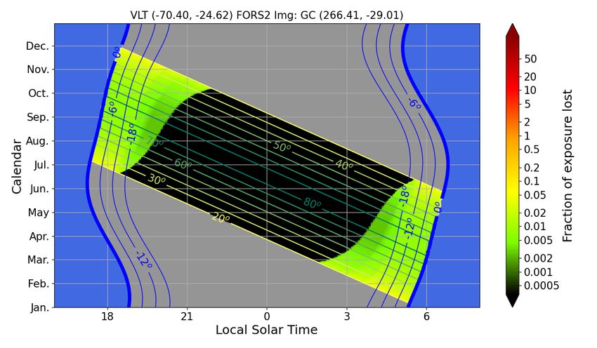
A&A proofs: manuscript no. satconsim

stellations, namely SpaceX’s Starlink and OneWeb, have already           Table 1. Orbit configurations for the satellite constellations considered
been placed in orbit. In Table 1 we list some of the planned             in this paper, totaling almost 60 thousand satellites, providing the orbital
                                                                         altitude and inclination, number of satellites within an orbital plane nsat
constellation configurations for which information is publicly           and the number of orbital planes nplane making up the constellation (con-
available. Several more satellite operators indicated their in-          sisting of nsat × nplane satellites). These are the constellations for which
tentions to build about a dozen of additional similar constella-         supporting information is available. These constellations are therefore
tions. Many companies are also planning constellations of much           to be considered as representative of a plausible situation by ∼ 2030,
smaller satellites (cubesats, nanosats...), which are less relevant      but the exact details of the distribution of satellites may be different.
for optical astronomy. We note that satellite operators, even those
with satellites already in orbit, frequently modify the configu-                Altitude    Inclination        nsat   nplane nsat × nplane
ration of their constellation projects. Furthermore, other satel-               Starlink Generation 1                     11926 satellites
lite operators have indicated their intentions to launch mega-                    550 km            53◦         22       72         1584
constellations, but without so far submitting any application or
                                                                                  540 km              53◦.2     22       72            1584
publishing any details. Therefore, the configurations used in this
                                                                                  570 km               70◦      20       36             720
paper should be treated as a representative, and their impact on
                                                                                  560 km              97◦.6     58        6             348
astronomical observations obtained from the following simula-
                                                                                  560 km              97◦.6     43        4             172
tions and their interpretation are an illustration of the situation as
                                                                                335.9 km               42◦      60       42            2493
it could be in the late 2020’s. In first approximation, the numbers
                                                                                340.8 km               48◦      60       42            2478
scale linearly with the total number of satellites in the constella-
                                                                                345.6 km               53◦      60       42            2547
tion, so the effects be scaled.
     Of all these projects, the SpaceX Starlink constellation is                Starlink Generation 2                    30000 satellites
clearly in the forefront. Since the launch of their first group of                328 km           30◦           1    7178         7178
satellites in May 2019, the trains of very bright pearls that form                334 km           40◦           1    7178         7178
the satellites illuminated by the Sun have caught the attention                   345 km           53◦           1    7178         7178
even of the general public, and have triggered the alarms of the                  360 km          96◦.9         50      40         2000
astronomical community (see, for example Witze 2019). These                       373 km           75◦           1    1998         1998
bright trains are formed only at the first stages of the deployment               499 km           53◦           1    4000         4000
of each Starlink launch, with the satellites becoming fainter as                  604 km          148◦          12      12           144
they later climb to the final operational orbits, and attain an op-               614 km         115◦.7         18      18           324
erational attitude that reduces their apparent brightness.                      Amazon Kuiper                              3236 satellites
     Our aim in this paper is to assess the impact of satellite mega-            630 km       51◦.9             34       34         1156
constellations on optical and near-infrared astronomy from com-                  610 km        42◦              36       36         1296
puter simulations of two kinds. Such simulations are described                   590 km        33◦              28       28           784
in §2, where we depict the usual discrete simulations and, also,
a new approach consisting on formulating statistical predictions                OneWeb Phase 1                             1980 satellites
from analytical probability density functions that describe the                 1200 km        87◦.9            55       36         1980
main properties of the constellations. The same section includes                OneWeb Phase 2 revised                     6372 satellites
consideration on how to estimate the apparent brightness of                     1200 km         87◦.9  49                36         1764
satellites illuminated by sunlight, with special attention to the               1200 km          40◦   72                32         2304
concept of effective magnitude.                                                 1200 km          55◦   72                32         2304
     The effect on observations is addressed in §3. There we pro-
vide details on the specific details of a set of simulations, their             GuoWang GW-A59                            12992 satellites
implications for several observing modes (direct imaging and                     590 km       85◦               60        8           480
spectroscopy, including multi-fiber instruments) and we discuss                  600 km       50◦               50       40         2000
some possibilities to mitigate the impact in §4. The appendix in-                508 km       55◦               60       60         3600
cludes the details on how the equations of our analytical model                 1145 km       30◦               64       27         1728
are derived.                                                                    1145 km       40◦               64       27         1728
                                                                                1145 km       50◦               64       27         1728
                                                                                1145 km       60◦               64       27         1728
2. Simulations
2.1. Visibility
                                                                         ulations presented here. Instead, we assume that the satellites
A satellite will be visible at optical and near-infrared wave-           move in circular Keplerian orbits, and we will neglect the ef-
lengths if it is above the horizon for the geographical location         fects of atmospheric drag, the lack of spherical symmetry of
of the observer and if it is illuminated by the Sun, making it to        the Earth’s gravitational potential and perturbations by the Sun
reflect and diffuse sunlight back to the observer. Hence, the visi-      and the Moon. Furthermore, for simplicity, satellite positions are
bility of a given satellite will depend upon its location within its     defined in an inertial geocentric reference system (Celestial In-
orbit, the geographic location of the observer, and the location of      termediate Reference System), neglecting the small effects of
the Sun, all as a function of time.                                      precession, nutation and Earth orientation parameters. These as-
     While the motion of a satellite in the Earth’s gravitational        sumptions allow us to consider only the idealised motion of the
field and through the higher residual layers of the atmosphere           satellites, the motion of the observer (uniform Earth rotation)
is usually computed through either numerical integration or us-          and the apparent motion of the Sun.
ing simplified analytical models (e.g. Montenbruck & Gill 2000;               Satellite constellations for worldwide coverage are generally
Vallado et al. 2006), these offer an accuracy that is not required       configured as Walker constellations (Walker 1984). Here, satel-
for the statistical results that we want to derive from the sim-         lites are in circular orbits of distinct orbital shells, with each
Article number, page 2 of 20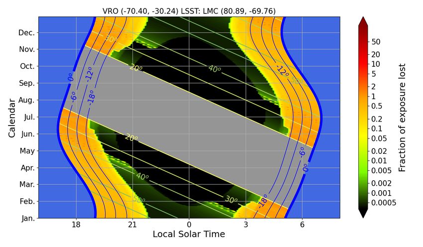
C. G. Bassa et al.: Analytical simulations of the effect of satellite constellations on optical and near-infrared observations

                                                     Starlink generation 2 at 2022-06-21T23:00:00

 60°N

 30°N

   0°

 30°S

 60°S
                                                                                                                             Sunlit
                                                                                                                             Eclipsed
                                                                                                                             Sunlit and above horizon
                                                                                                                             Sunlit and above horizon
                                                                                                                             Rubin Observatory
                                                                                                                             London
    180°                   120°W                   60°W                     0°                    60°E                   120°E                      180°

Fig. 1. A discrete realization of the Starlink Generation 2 constellation overlaid on a map of Earth. The day and night sides of Earth are shown
for 2022 June 21 at 23:00UTC, near the June solstice. Satellites are shown as either sunlit (yellow), or eclipsed by the Earth (black) and above
the horizon for two geographical locations, Vera Rubin Observatory in Chile (latitude −30◦ ), and London in the United Kingdom (latitude ∼ 50◦ ).
Over-densities of satellites in geographic latitude b are visible at latitudes |b| = 30◦ , 40◦ and 53◦ , corresponding to the inclination of the most
populous orbital shells. Due to their orbital altitudes, satellites remain visible for locations where the Sun is below the horizon, and will remain
visible throughout all the night for locations at high geographical latitudes.

shell described by its orbital altitude hsat and orbital inclination        2.1.1. Discrete simulations
i. Within each shell, equally spaced orbital planes are populated
by satellites, also equally spaced within each plane. In Table 1            To obtain a realization of a satellite constellation at a given
we use nsat to denote the number of satellites in a single orbital          time, the positions and velocities of all satellites in the constella-
plane, and nplane to indicate the number of orbital planes. The to-         tion are computed using the assumptions listed earlier. Figure 1
tal number of satellites within each shell is Nsat = nsat × nplane ,        shows such a realization for the Starlink Generation 2 constella-
and the total number of satellites in a constellation the sum of            tion on a map of the Earth near the June solstice when the Sun is
the number of satellites in each shell.                                     at its highest northern declination. Hence, for locations at high
                                                                            geographical latitudes in the northern hemisphere, satellites will
                                                                            be visible throughout the whole night, whereas for lower lati-
    In this paper we consider only idealized, complete constel-             tudes and in the southern hemisphere satellites will only be vis-
lations. Individual satellites, as well as the trains of satellites         ible around twilight. This figure depicts over-densities of satel-
in very low orbits right after launch and the satellites in near-           lites at geographical latitudes near the orbital inclination of dif-
to-re-entry orbits, are not considered. Even taking into account            ferent orbital shells.
the large number of launches required to replenish the constel-                  These over-densities are also seen in the all-sky maps shown
lations, and the hopefully equally large number of satellites on            in Fig. 2 for two locations, the Vera Rubin Observatory (VRO)
end-of-life orbits, the number of such satellites will be one to            at Cerro Pachón in Chile (at latitude −30◦ ), and London in the
two orders of magnitude smaller than the number of satellites in            United Kingdom (at latitude +50◦ ). The increased distance to the
operations. Also, as these satellites are in lower orbits their im-         orbital shells when looking at lower elevations above the horizon
pact is concentrated during the very beginning and end of night.            leads to larger sampling volumes, which explains that these all-
Hence, their contribution to the overall situation caused by the            sky maps show increasing satellite densities towards the horizon,
constellations in operation is therefore small.                             though additional over-densities exist near the projected location
                                                                            of the northern and southern limits of the most populous orbital
    We expand on the work by Hainaut & Williams (2020), who                 shells.
used a simplistic geometric approximation to estimate the den-                   This discrete approach has been followed to assess the im-
sity of satellites and their effects. That model had the advantage          pact of satellite constellations in terms of the amount of them
of being extremely fast and numerically lean, and to yield ac-              that are visible during the night above a given elevation from
ceptable results for mid-latitude observatories, but it had the ma-         the horizon, as shown, for instance, in McDowell (2020). To this
jor shortcoming not to account for latitude effects. This aspect is         end, a specific constellation is selected (in terms of shell number
rigorously addressed in the following sections.                             and, for each of them, the altitude, orbital inclination and num-
                                                                                                                        Article number, page 3 of 20
A&A proofs: manuscript no. satconsim

                          Rubin Observatory                                                                    London
                                     N                                                                              N

 E                                                                       W E                                                                          W

         Sunlit
         Eclipsed
                                     S                                                                              S
Fig. 2. A discrete realization of the Starlink Generation 2 constellation plotted on all sky maps representing the sky above Vera Rubin Observatory
(left) and London (right). Satellites are shown as sunlit (yellow) or eclipsed by the Earth (black). The number of satellites increases towards the
horizon because, for a given solid angle, looking at lower elevations from the horizon the distance to the shell surface increases and, hence, the
field of view contains larger portions of the orbital shells. Due to the orbital inclination and orbital altitude of the orbital shells, over-densities of
satellites are also present in these maps. The map for London shows this very clearly for the two orbital shells with i = 53◦ and h = 345 km (7178
satellites) and 499 km (4000 satellites), where more satellites are present south from the dotted line. The dotted line in the all sky map for Vera
Rubin Observatory is for the orbital shell with i = 30◦ , h = 328 km, with a larger number of satellites north from that line.

ber of satellites), an observatory location is specified (in general          an observer at −30◦ latitude, the number of satellite trails visible
only latitude is relevant) and the illumination conditions are fixed          within an observation of an exposure time and circular field-of-
through Sun declination and hour angle. The simulation of the                 view towards zenith were counted and averaged over 1000 sim-
Keplerian movement of each satellite of the constellation allows              ulations.
counting the number of satellites that are above a specific ele-                  The simulations show a dependence with both field-of-view
vation and their illumination conditions (sunlit or eclipsed). Ad-            and exposure time (solid dots). This relation can be understood
ditional considerations may allow computing some photometric                  as the number of satellites present at the start of the exposure,
estimates (§2.2). This kind of discrete, all-sky simulations may              plus those travelling through the field-of-view during the expo-
be iterated, including some random initialisation of parameters               sure, and has the form
at each run to average-out systematic effects due to the spatial
and temporal texture induced by the constellation structure.                  Ntrail = ρsat (Afov + Lfov ωsat texp ).                                 (1)

                                                                              Here, ρsat is the instantaneous satellite number density, i.e. the
2.1.2. Number of satellite trails in an observation                           number of satellites per unit area on the sky, and ωsat the angular
                                                                              velocity of the satellites in the direction of the exposure. The
Besides the all-sky simulations, an observation-oriented ap-                  exposure itself has field-of-view area of Afov and width Lfov , and
proach is also needed. This requires specifying all the param-                exposure time teff . For comparison with the simulations we use
eters required for the all-sky simulations and, also, selecting the           a field-of-view with a circular radius Rfov , such that Afov = πR2fov
observation direction (azimuth, elevation), field-of-view (FOV)               and Lfov = 2Rfov .
and exposure time of an observation. In these observations, the                    The simulations provide the instantaneous satellite density
motion of the satellite during the exposure will leave a satellite            ρsat and the average angular velocity ωsat and using these values,
trail on the images. Repeating this simulation leads to the aver-             Eqn. 1 provides the predicted number of trails for the different
age estimate of the number of satellite trails that would affect              observation parameters, plotted as lines in Fig. 3. The predictions
the observation. The geometry of the problem allows also com-                 match the simulations, though for short exposures and/or small
puting the position angle of the trails and the apparent angular              fields-of-view, the simulations suffer from noise due to the few
velocity of each satellite that crosses the FOV.                              satellites passing through the observation.
     In Fig. 3 we show the results of a discrete simulation on ob-                 Equation 1 is valid for a single shell in a constellation, as the
servations with different exposure times and fields-of-view. The              instantaneous density ρsat and angular velocity ωsat depend on
discrete simulation used a constellation of 10 000 satellites in              the properties of the shell. To obtain the total number of trails in
a single orbital shell of 100 orbital planes with 100 satellites              an observation for a satellite constellation with multiple shells,
within each plane, at 1000 km altitude and 53◦ inclination. For               Eqn. 1 can be computed for each shell, and the results summed.
Article number, page 4 of 20
C. G. Bassa et al.: Analytical simulations of the effect of satellite constellations on optical and near-infrared observations

                             100                                                                        that it removes any dependence on the precise shape and orienta-
                                         1 deg2        20 deg2
                                         2 deg2        50 deg2                                          tion of the instrument field-of-view, and instead solely depends
                                         5 deg2        100 deg2                                         on the sky area covered by the field-of-view. The assumption
                              10         10 deg2                                                        allows us to evaluate Eqn. 2 for a line-of-sight (specified by az-
                                                                                                        imuth and elevation) of the observation from an observatory on
Number of satellite trails

                                                                                                        Earth intersecting the orbital shell at distance d and with an im-
                               1                                                                        pact angle α (α = 90◦ at zenith and α < 90◦ for lower ele-
                                                                                                        vations). The instantaneous surface density ρsat can then be ob-
                                                                                                        tained by scaling the probability by the surface area of the orbital
                                                                                                        shell covered an angular area A of 1 square degree, providing
                              0.1

                                                                                                                                 d2 A
                                                                                                        ρsat = Nsat P(φ, i, hsat )    ,                                      (3)
                             0.01                                                                                               cos α
                                                                                                        where Nsat is the number of satellites in the orbital shell with
                                    1                10                100           1000               inclination i and orbital altitude hsat . Equations to derive the dis-
                                                            Exposure time (s)                           tance d and impact angle α given the location of the observatory
                                                                                                        and azimuth and elevation of the observation are given in Ap-
Fig. 3. The number of satellites visible in an exposure depending on                                    pendixes A.2 and A.3.
the exposure time texp , and the instrument field-of-view, specified by                                      The angular velocity of the satellites in an orbital shell to-
its circular radius Rfov = L/2. The effect of a discrete constellation of
                                                                                                        wards the line-of-sight can be determined using the equations
10 000 satellites in a single orbital shell of 100 orbital planes and 100
satellites per plane at 1000 km altitude and 53◦ inclination is simulated                               provided in Appendix A.4. Due to the rotation of the Earth within
for an observer at −30◦ latitude, observing towards zenith. The points                                  the orbital shell of a satellite constellation, the velocity vectors
are the results of the discrete simulations for different values of exposure                            project differently on the sphere of the sky and hence satellites
time texp and field-of-view (πR2fov ). The solid lines are predictions based                            will have somewhat different angular velocities depending on
on Eqn. 1.                                                                                              their north- or southbound trajectory. Given that for a full con-
                                                                                                        stellation, an equal amount of satellites will be on northbound as
                                                                                                        well as southbound trajectories, we can take the average of both
2.1.3. Analytical simulations                                                                           angular velocities to obtain ωsat .
The averaging over many randomly initialized parameters of a                                                 For a given satellite constellation, observatory latitude and
satellite constellation for the discrete simulations is computa-                                        observation parameters (field-of-view and exposure time), the
tionally expensive, and may lead to noise due to insufficient                                           analytical simulations predict the number of trails as a function
satellites passing through observations with small fields-of-view                                       of azimuth and elevation which is inherently static with time.
and/or short exposures to obtain a valid average (see Fig. 3).                                          The final step to complete the analytical simulation is taking
Given that the averaging over randomly initialized parameters                                           into account the illumination of the different orbital shells by
has the effect of smoothing out the satellite locations within a                                        the Sun, as this modulates the visibility of a shell as a function
given orbital shell, we instead treat the satellite locations as prob-                                  of time of day and time of year. The impact of solar illumination
ability density functions, which have the advantage that these are                                      is implemented by computing whether the intersection of a given
analytical expressions.                                                                                 line-of-sight with an orbital shell is in the shadow of the Earth
     Figure 1 shows that the satellite locations are uniformly                                          or not. If the intersection point is located in the shadow, and the
spread in geocentric longitude, but strongly peaked towards geo-                                        satellites are not visible, we set Ntrail = 0 for that shell in the sum
centric latitudes φ close to the values equal to the orbital incli-                                     of satellite trails over the different orbital shells.
nation −i and +i of a constellation shell. For a satellite at true                                           Figure 4 shows all sky maps using the analytical simulations,
anomaly (measured from the ascending node) κ, the geocentric                                            providing the number of satellite trails from Eqn. 1. The contri-
latitude is given by sin φ = sin κ sin i, and its probability distri-                                   bution of the different orbital shells of multiple satellite constel-
bution follows the Arcsine probability distribution1 . For a single                                     lations is apparent, as is the impact of solar illumination.
satellite at orbital altitude hsat , the probability density per unit
surface area as a function of φ is:                                                                     2.2. Photometry
                                                                    1
 P(φ, i, hsat ) =                                                                           .    (2)    Providing a reliable estimation of the apparent brightness of the
                                           2π2 (R⊕ + hsat )2 (sin i + sin φ)(sin i − sin φ)
                                                            p
                                                                                                        satellites is an obvious requirement for any model that intends
Here R⊕ is the radius of the Earth, and this expression is valid                                        to assess the impact of mega-constellations on astronomical ob-
for |φ| < i, and zero otherwise. A detailed derivation of Eqn. 2 is                                     servation. The celestial mechanics part of the problem admits an
given in Appendix A.1.                                                                                  accurate solution that, even in a simplified frame (as described in
    Equation 2 can be integrated over the surface of the orbital                                        §2.1.1 and §2.1.3), leads to sound predictions of the spatial pa-
shell spanned by the field-of-view of an instrument from an ob-                                         rameters (satellite density and their motion). However, the pho-
servatory located on Earth to obtain the fraction of the sam-                                           tometric part of the problem faces additional difficulties, due to
ple present within the instrument field-of-view. For the remain-                                        the complex geometrical and reflective properties of the satellite
der of the paper, we will make the simplifying assumption that                                          that, also, are different from one constellation to another.
P(φ, i, hsat ) is constant over the instrument field-of-view. This as-                                      In the visible and near-infrared (NIR), the light from the
sumption will generally be true for the small fields-of-view un-                                        satellite is reflected sunlight with a specular and a diffuse com-
der consideration in the remaining analysis. It has the advantage                                       ponent. The specular reflection happens on flat panels: anten-
                                                                                                        nas, satellite bus, possibly also solar panels (although while the
     1
                        https://en.wikipedia.org/wiki/Arcsine_distribution                              satellites are in operations, these are perpendicular to the Sun).
                                                                                                                                                    Article number, page 5 of 20
A&A proofs: manuscript no. satconsim

                                                                                                      0
                                                                                                                                     Alt. 350km
                                                                                                      1                              Alt. 550km
                                                                                                                                     Above 550km
                                                                                                      2

                                                                            Satellite magnitude [V]
                                                                                                                                     Below 550km

                                                                                                      3

                                                                                                      4

                                                                                                      5

                                                                                                      6

                                                                                                      7

                                                                                                      8
                                                                                                          400   600     800        1000      1200
                                                                                                                      Range [km]

                                                                            Fig. 5. Magnitude of the satellites as a function of the range observer-
                                                                            satellite. The dots are measurements of original Starlink satellites
                                                                            (Pomenis telescope, from Otarola et al. 2020), and the lines are obtained
                                                                            using a simplified Lambertian sphere model for two altitudes. The un-
                                                                            known solar phase angle contributes to the dispersion of the measure-
                                                                            ments.

Fig. 4. Sky maps with an example of the resulting number of trails per      object’s intrinsic photometric properties: pR2sat is the photomet-
exposures. The circles mark 0◦ , 10◦ , 20◦ , 30◦ , and 60◦ elevation. The   ric cross-section, with p the object’s geometric albedo and Rsat
observatory is located at +50◦ latitude; the sun at −18◦ elevation; the     the radius of the (spherical) satellite. The third term includes sev-
camera has a FOV with diameter Lfov = 60 , and the exposure time is         eral distances: dsat is the distance from the satellite to the Sun,
300 s. The satellites are those from Table 1. In the black region at the    dsat represents the distance from the observer to the satellite. For
South-East, all satellites are already in the shadow of the Earth. The      our problem, dsat = 1 AU. The fourth term is the correction for
edges running from North-East to South-West correspond to constel-          the solar phase α . Finally, kχ represents the extinction term, k
lation shells at lower altitudes, whose South-East parts are already in     being the extinction coefficient (in magnitudes per unit airmass),
the shadow. The sharp features running from East to West correspond
to the edges of constellation shells whose inclinations are close to the
                                                                            and χ the airmass (equal to 1/ sin esat in the plane-parallel ap-
observatory latitude.                                                       proximation, with esat representing the satellite’s elevation above
                                                                            the horizon; here, as we know the orbits of the object, we use the
                                                                            exact χ = dsat /hsat ). In the V band, k = 0.12 is a typical value
A complete and accurate representation of the reflection by a               (Patat et al. 2011).
satellite would require detailed knowledge of the shape and ma-                  For a Lambertian sphere, υ(α ) = (1 + cos α )/2. However,
terial of the satellites (see Walker et al. 2020, for a summary of          a large number of photometric measurements of Starlink origi-
the state-of-the-art). A simplified model can be assembled from             nal satellites (Mallama 2020b) and Starlink VisorSat (Mallama
photometric observations covering a range of zenithal distance              2021) indicate an extremely weak dependency of the magnitude
and solar illumination.                                                     (corrected for distance and extinction) with the solar phase an-
    Empirical models (for instance, a flat panel model, Mallama             gle, a circumstance that has to be related to the morphology of
2020a) are being developed, and theoretical approaches are also             the satellite, which is very different to a sphere. We therefore
used to define photometric parameters of the satellites (Walker             consider υ = 1, leading to
et al. 2020). However, as of today, the available observations
are sufficient only for simplistic photometric models. Hopefully,           msat = m + 2.5 log10 dsat 2
                                                                                                         − 2.5 log10 pR2sat + kdsat /hsat ,   (5)
dedicated observation campaigns will refine the characterization
of the satellites in the coming years.                                      where both dsat and Rsat are expressed in the same units.
                                                                                The photometric cross-section is the only parameter that de-
2.2.1. Apparent magnitude                                                   pends on the satellite’s physical properties in this model. Hain-
                                                                            aut & Williams (2020) adopted pR2sat = 0.25 m2 for the first-
The simple photometric model we use is based on the Lamber-                 generation Starlink. In order to facilitate the comparisons be-
tian sphere model. The theoretical foundations of the Lamber-               tween satellites, one introduces the absolute magnitude m1000km ,
tian sphere model can be seen, for instance, in Karttunen et al.            normalized to a standard distance dsat = 1000 km. With that
(1996). The different specific formulations, such as those by               value for dsat , Eqn. 5 becomes
Hainaut & Williams (2020) and McDowell (2020), can be uni-
fied under a single formula:                                                msat = m1000km + 5 log10 (dsat /1000) + kdsat /hsat ,                   (6)

                                                                            with dsat expressed in km. Sometimes, m550km = m1000km − 1.3 is

msat = m − 2.5 log10 pR2sat + 5 log10 (dsat dsat )
                                                                            used instead.
           −2.5 log10 υ(α ) + kχ .                                   (4)
                                                                                Table 2 lists the absolute magnitudes measured for different
   In Eqn. 4, m is the Sun’s apparent magnitude as seen from                satellite types, and the corresponding photometric cross-section
Earth, in the photometric band of interest. Typically, this is John-        and visual magnitude at zenith. The dispersion of the measure-
son’s V band, with m = −26.75. The second term considers the                ments of m1000km is around 0.7 mag; Fig. 5 shows an even wider
Article number, page 6 of 20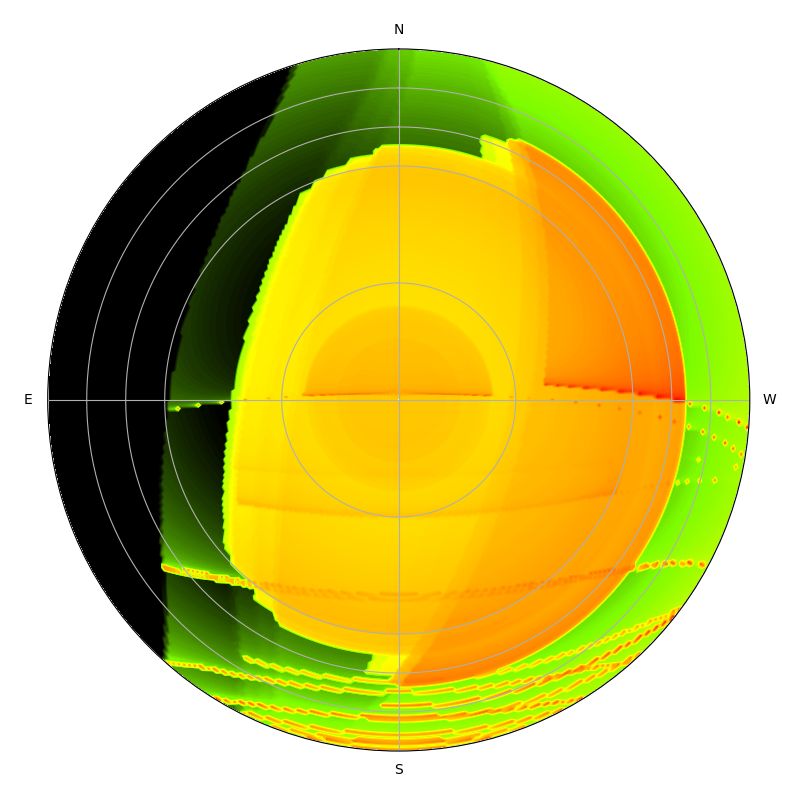
C. G. Bassa et al.: Analytical simulations of the effect of satellite constellations on optical and near-infrared observations

Table 2. Representative magnitudes of the satellites.

 Satellite               Operational Mag      Mag              Mag          pr2      p       r       Ref.
                         altitude    at op. dispersion at
                         [km]        alt.                      1000km [m2 ]                  [m]
 Starlink original       550km       4.6      0.7              5.9          0.085 0.25 0.58 1
                                     4.0      0.7              5.3          0.152 0.25 0.78 2
                                     4.2      (model)          5.5          0.125 0.25 0.71 3
 Starlink DarkSat 550km              5.1      (single)         6.4          0.056 0.08 0.71 4
 Starlink VisorSat 550km             6.2      0.8              7.5          0.023 0.25 0.30 5
                                     5.8      0.6              7.1          0.028 0.25 0.33 6
 OneWeb              1200            7.6      0.7              7.2          0.027 0.25 0.33 7
Notes: p is the (arbitrary) geometric albedo used for the conversion of the cross-section pr2 into an estimate of the radius r.
References: 1: Mallama (2020b); 2: Krantz in Otarola et al. (2020); 3: value used in Hainaut & Williams (2020); 4: using the darkening of 0.88
mag on one DarkSat, from Tregloan-Reed et al. (2020); 5: median value from Mallama (2021); 6: average from Krantz in Otarola et al. (2020); 7:
Mallama (2020c)

                                                                             worth noting that the dependency of meff with the altitude of the
                                                                             satellites is shallower than that of the apparent magnitude.
                                                                                 In this approximation we are assuming that the satellite’s
                                                                             PSF has the same shape as the stellar PSF at the telescope fo-
                                                                             cal surface, a crude approximation if the distance to the satellite
                                                                             is small enough for it to be spatially resolved, or out of focus, or
                                                                             both (Tyson et al. 2020; Ragazzoni 2020). The apparent angular
                                                                             width of the satellite trail is
                                                                                             D2sat + D2m
                                                                             θsat
                                                                              2
                                                                                  = θatm
                                                                                     2
                                                                                         +         2
                                                                                                         ,                                          (8)
                                                                                                 dsat
                                                                             where θatm is the stellar FWHM (the seeing, typically ∼ 000. 8
                                                                             from a good site), Dsat the physical diameter of the satellite, Dm
                                                                             the diameter of the telescope mirror, and dsat the distance to the
                                                                             satellite (Tyson et al. 2020). For an 8-m telescope like the ESO
Fig. 6. Visual (red) and effective magnitudes of a satellite at zenith, as   Very Large Telescope (VLT), or the Simonyi Survey Telescope
a function of its altitude, for various exposure times (see legend). The
                                                                             (formerly LSST), a 2 m satellite at an altitude of 300 to 550km,
satellite used is a Starlink VisorSat with m1000km = 7, considered as a
trailed point source.                                                        θsat ∼ 600 to 300 . The spreading of the signal from the satellite
                                                                             over this larger area will decrease its signal-to-noise ratio (SNR)
                                                                             by up to θsat /θatm , and its peak intensity by up to (θsat /θatm )2 , i.e.
dispersion. Consequently, the simplistic model presented above               2 to 4 magnitudes fainter than meff from Eqn. 7.
can only represent the general trend of the satellite magnitude, as               For imaging, the resolution element is typically the seeing
illustrated by the comparison with observations (Fig. 5). In the             (of the order of 100 ) for telescopic observations, or the pixel (a
simulations described below, we will use m1000km = 7, equivalent             few to a few tens arcsec) for wide-field astrophotography. Fig-
to m550km = 5.7.                                                             ure 7.a displays the visual magnitude of the faintest satellite that
                                                                             will leave a trail with SNR = 5 as a function of the limiting mag-
                                                                             nitude, for texp = 60 s imaging observations. This shows that all-
2.2.2. Effective magnitude and limiting magnitude                            sky cameras will record only the brightest satellites and flares.
During an exposure of duration texp , a satellite will leave a trail of      Only the deepest wide-field astrophotography (with a limiting
length ωsat texp (with ωsat being the apparent angular speed of the          magnitude V ∼ 15 in texp = 1 min or fainter) will record the bulk
satellite), typically much longer than the FOV of the instrument.            of the satellites. Telescopic observations are fully affected by all
The signal corresponding to the apparent magnitude is therefore              most satellites.
spread along the length of the trail. The count level on the detec-               The situation is slightly different for spectroscopy. In the case
tor amounts to the light accumulated inside an individual resolu-            of fibre-fed spectrographs, the resulting data contain no spatial
tion element (whose size is r) during the time teff = r/ωsat that            information at all; for long-slit spectrographs, the spatial infor-
the satellite takes to cross that element. This leads to the con-            mation is available in only one direction. Except in the case of
cept of effective magnitude, meff , defined as the magnitude of a            integral-field spectrographs, the data will therefore not include a
static point-like object that, during the total exposure time texp ,         tell-tale trail indicating the contamination. For an exposure time
would produce the same accumulated intensity in one resolution               texp = 1200 s, representative of individual exposures in the vis-
element than the artificial satellite during a time teff :                   ible, Fig. 7.b displays the visual magnitude of the satellite that
                                                                             will reach a SNR = 5 as a function of the limiting magnitude.
                          teff                       r                       Spectrographs having a limiting magnitude brighter than V = 20
meff = msat − 2.5 log10        = msat − 2.5 log10           .         (7)    in texp = 1200 s will essentially be immune: the signal from a
                          texP                    ωsat texp
                                                                             satellite will be be too faint to be detected. That will be the case
Figure 6 shows the effective magnitude for an example. While                 for low-resolution spectrographs on small to medium telescopes,
not directly relevant for low-altitude constellation satellites, it is       and high-resolution spectrographs on large telescopes.
                                                                                                                         Article number, page 7 of 20
A&A proofs: manuscript no. satconsim

a
                                                                                 3200
                                                                                               Summer                                                          Winter
                                                                                 2800
                                                                                                                                            Above horizon
                                                                                 2400
                                                                                 2000

                                                                                                    Sunset
                                                                                 1600

                                                                                                             -12o
                                                                                                             -18o
                                                                                                      -6o
                                                                                 1200
                                                                                  800
                                                                                  400
                                                                                   0
                                                                                        16    18             20          22           24        26        28        30   32
                                                                                  350

                                                                                  300                                                       Above 30o
                                                                                  250

                                                                                  200

                                                                                  150

                                                                                  100

                                                                                   50

                                                                                   0
                                                                                              18                    21                 0             3              6
                                                                                                                          Local solar time
b                                                                                                  All Satellites             Illuminated       mag < 6        mag < 5

                                                                                Fig. 8. Number of illuminated satellites above the horizon (top panel)
                                                                                and above 30◦ elevation, as a function of the local solar time, for Paranal
                                                                                (latitude −24◦.6), accounting for all the satellites from Table 1. Left is
                                                                                for the summer solstice (δSun = +23◦.4), and right for the winter sol-
                                                                                stice (δSun = −23◦.4). The twilights are indicated with blue shading.
                                                                                The black line marks the total number of satellites above the elevation
                                                                                considered, the blue line those that are illuminated, and the orange and
                                                                                red lines those brighter than magnitude 6 and 5, respectively, using the
                                                                                photometric model described in §2.2.

                                                                                contamination. However, if the target was a stellar object, a solar
                                                                                contamination might cause spurious conclusions.

                                                                                3. Results
                                                                                3.1. Time and Solar declination dependence
Fig. 7. Detection limit for the satellite apparent magnitude as a function
of the limiting magnitude of the instrument. a: the for an imager, the          The analytical models for visibility and photometry allow us to
limiting magnitude corresponds to 5σ in a 60s exposure time; b: for a           compute their dependence on time of day as well as time of year.
spectrograph, the limiting magnitude corresponds to 5σ in a 1200s ex-           Similar results were already presented using a simplified geo-
posure. In both cases, various resolution element sizes are represented         metric model by Hainaut & Williams (2020), or discrete sim-
in different colour. Typical satellite apparent velocities corresponding to     ulations by McDowell (2020). Figure 8 shows the number of
various elevations are represented with different line styles. A satellite
                                                                                satellites illuminated by the Sun for the local summer and winter
will be detected if its apparent magnitude is in the shaded area above
the coloured line corresponding to the considered elevation. The hori-          seasons for an observatory at latitude −24◦.6. During local sum-
zontal limit correspond to the typical brightest satellite at that elevation.   mer, satellites remain visible above 30◦ elevation throughout the
Typical limiting magnitudes are indicated.                                      night. Figure 9 shows the visibility dependence as a function of
                                                                                solar elevation, for each shell (exposing the importance of the
                                                                                shell altitude) and for the total populations from Table 1.

    If the SNR of the contamination is much lower than that of                  3.2. Spatial fine structure
the science target, the contamination will result in a small in-
crease of the background noise, what can probably be neglected                  An outstanding effect of the orbital shells of satellite constel-
for most science cases. Also, cases where the SNR of the con-                   lations is the amount of spatial fine structure that arises in the
tamination is much larger than that of the science spectrum are                 quantity of satellites visible on the local celestial sphere, as il-
trivial: the effect is obvious and the observation is lost. The situ-           lustrated in Fig. 2 and Fig. 4. Of course, first of all we find the
ation for spectrographs with a limiting magnitude in the v = 20–                effect of the Earth’s shadow, whose behaviour is, as expected,
23 range in texp = 20 min is more problematic: the satellite trail              dominated by the diurnal rotation of the planet and by the inter-
will have a SNR of 2–15, so that contamination caused by the                    play between observatory latitude and Sun declination. But the
satellite will be at a level comparable to that of the science sig-             structure of satellite shells, combined with orbital mechanics,
nal. It is therefore plausible that the contamination will not be               adds a far from negligible spatial fine structure in the quantity
immediately apparent, and will be discovered only at the time                   of satellites visible on the local celestial sphere. In particular,
of the data analysis, where a solar-type spectrum (reflected by                 as Eqn. 2 shows, each individual shell induces an unavoidable
the satellite) will be superimposed to that of the science target.              over-density high in the sky over observatories placed at geo-
These intermediate cases where both SNRs are similar are much                   graphic latitudes φ whose absolute value is close to the orbital
more problematic and science-case dependent: if the science tar-                inclination i. The Northern or Southern boundary of each shell
get is a distant galaxy, a solar spectrum will be identified as a               lies along a line on the local celestial sphere that crosses zenith
Article number, page 8 of 20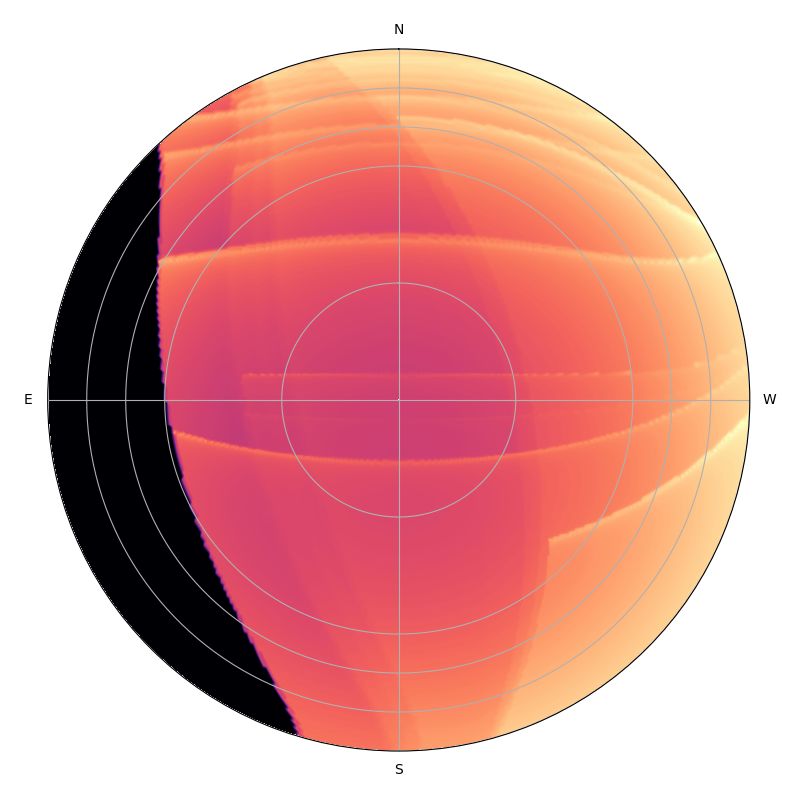
C. G. Bassa et al.: Analytical simulations of the effect of satellite constellations on optical and near-infrared observations

                                                                             a

Fig. 9. Number of illuminated satellites above the horizon as a function
of the Sun elevation, for the constellations listed in Table 1 seen from
Paranal (latitude −24◦.6; the dependency with latitude is not strong). The
twilights are indicated with blue shadings, and the elevation of the sun
at midnight by grey shadings for the solstices and equinoxes. The thin
lines represent the individual shells, and the thick lines the totals for
each constellation. The upper thick black line is the grand total.

if φ = i, what incidentally happens for Vera Rubin Observatory               b
and some shells currently considered in several constellation de-
signs. These over-densities may coincide with the culmination
elevation of some key objects (let us say, for instance, LMC or
SMC in the South, or M31 and M33 in the North). Given the
inclination i of one orbital shell and the latitude φ of the obser-
vatory, the shell boundary cuts the local meridian at a declination
δ that can be deduced from the following equation (justified in
Appendix A.5):
                R⊕ + hsat
sin (δ − φ) =             sin (δ − i)                                 (9)
                   R⊕

3.3. Contribution to the sky brightness
The satellites, including those that are not directly detected, con-
tribute to the sky background. To evaluate this effect, surface
brightness maps were computed. The magnitude of a satellite
from a constellation was evaluated using Eqn. 6, then converted
into flux, and finally used to weight the satellite density map
described in §2.1.3. A total flux density map was obtained sum-
ming the contributions of all satellite shells, and transformed into
surface brightness in mag/sq.arcsec. An example is presented
in Fig. 10. In the illuminated part of the shells, the satellites
contribute to a surface brightness in the 28–29 mag/sq.arcsec
range (0.3–0.7 µcd m−2 ), with peaks around 26.5 mag/sq.arcsec               Fig. 10. Sky brightness contribution from the satellites (using the con-
(2.7 µcd m−2 ) at the cusps of the constellations. The surface               stellations from Table 1), at astronomical twilight at latitudes +50◦
brightness of the dark night sky is around V = 21.7 (Patat 2008)             (a) and −25◦ (b). Typical sky surface brightness in the visible is 21.7
(225 µcd m−2 ), which means that the satellites from Table 1 will            mag/sq.arcsec or brighter. The satellites used all have v1000km = 7, re-
contribute at most an additional ∼ 1% to the sky brightness in               sulting in visual magnitudes in the range indicated at the bottom right
the worst areas of the sky. The contribution to the sky brightness           corner.
is therefore small, and the simulations and mitigation focus on
the discrete contamination by individual satellites.
    Kocifaj et al. (2021) have evaluated the increase in diffuse
sky brightness caused by all current space objects with sized be-
tween 5 × 10⁻⁷ m to 5 m at altitudes above 200 km. They esti-
mate that this excess is 16.2 µcd m−2 (24.6 mag/sq.arcsec) and               i.e. space debris. The macroscopic satellites composing the con-
can reach 21.1 µcd m−2 (24.3 mag/sq.arcsec)at astronomical twi-              stellations discussed in this paper will not contribute much to the
light, corresponding to about 10% of the natural sky brightness.             diffuse sky brightness provided they are not ground into micro-
That excess is dominated by the small objects (mm and below),                scopic debris.
                                                                                                                        Article number, page 9 of 20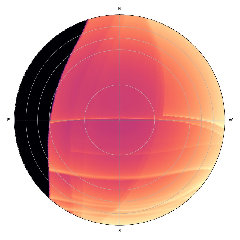
A&A proofs: manuscript no. satconsim

Table 3. Characteristics of instruments and exposures used for the simulations.

    Inst. Tel. Obs.          l          D                Field          texp [s]   r [arcsec]   Mag.
    Visible and near-IR Imagers
    EFOSC NTT ESO −29◦.25               3.6      Vis     40                300     1            24.2      Focal reducer (Buzzoni et al. 1984)
    (La Silla)
    FORS VLT ESO −24◦.6                 8.2      Vis     60                300     0.8          25.2      Focal reducer (Appenzeller et al.
    (Paranal)                                                                                             1998)
    HAWKI VLT ESO −24◦.6                8.2      NIR     7.5
                                                          0                 60     0.6          21.4      Near-IR imager (Kissler-Patig et al.
    (Paranal)                                                                                             2008)
    MICADO ELT ESO −24◦.6               39.      NIR     5000               60     0.015        24.9      Visible and near-IR imager with
    (Armazones)                                                                                           adaptive optics on the ELTa

    OmegaCam       VST       −24◦.6     2.4      Vis     1.0◦              300     0.8          23.9      Survey wide-field imager (Kuijken
    ESO (Paranal)                                                                                         et al. 2002)
    1.5m Catalina U.AZ          32◦.4   1.52     Vis     2.2◦               30     1.5          21.4      Survey wide-field imagerb
    (Mt. Lemmon)
    LSST Cam. SST            −30◦.2     8        Vis     3.0◦               15     0.8          24.6      Survey wide-field imagerc
    VRO (Pachon)
    0.7m Catalina U.AZ          30◦.4   0.7      Vis     4.4◦               30     3            19.8      Survey wide-field imagerb
    (Mt. Bigelow)
    Photo                     −30◦      0.07     Vis     75◦ × 55◦          60     60           10        Photographic camera with a wide-
                                                                                                          angle lens from a good site.
  Visible and near-IR Spectrographs
  FORS VLT ESO −24◦.6 8.2                       Vis     60 × 100        1200 0.8              22.0    Long-slit low-resolution spectro-
  (Paranal)                                                                                           graph (Appenzeller et al. 1998)
  UVES VLT ESO −24◦.6 8.2                       Vis     1000 × 100      1200 0.8              17.0    High-resolution echelle spectro-
  (Paranal)                                                                                           graph (Dekker et al. 2000)
  4MOST-L         VISTA −24◦.6 4                Vis     4◦.1            1200 0.8              20.5    Multi fibre1 spectrograph (low res.)
  ESO (Paranal)                                                                                       (de Jong et al. 2016)
  4MOST-H VISTA −24◦.6 4                        Vis     4◦.1            1200 0.8              18.6    Multi-fibre1 spectrograph (med
  ESO (Paranal)                                                                                       res.) (de Jong et al. 2016)
  ESPRESSO          VLT −24◦.6 8.2              Vis     000. 5          1200 0.5              15.8    High-resolution echelle (Pepe et al.
  ESO (Paranal)                                                                                       2021)
  Thermal IR
  VISIR VLT                  −24◦.6 8.2        ThIR 6000                  10 000. 2           –       Imager (Lagage et al. 2004)
  METIS ELT                  −24 .6 39
                                 ◦             ThIR 10       00
                                                                          10 000. 03          –       Adaptive Optics Imager on ELTd,2
l: latitude; D: diametre of the telescope; Field: field of view of the instrument; texp : exposure time [s]; r: resolution element [arcsec];
Mag: 5σ limiting magnitude for a point source for an exposure of duration texp .
References: a, https://elt.eso.org/instrument/MICADO/ - b, https://catalina.lpl.arizona.edu/about/facilities/
telescopes - c, https://www.lsst.org/about - d, https://elt.eso.org/instrument/METIS/
Notes: 1: 4MOST is a multi-object spectrograph equipped with 2436 fibres. Monte-Carlo simulations showed that, on average, a
satellite crossing the field of view will affect 1.3 fibres. 2: METIS also has a high-resolution spectrograph.

3.4. Effect on observations                                               and Lfov = L1 in the second term of Eqn. 1 – this maximises
                                                                          the cross-section for trails. Nsat was computed for each shell ac-
To evaluate in more detail the effects of satellite constellations on     counting for the effective magnitude of the satellites in that shell.
observations, we studied a series of representative instruments
and telescopes. For each of them, we consider the field of view               The effect on the observations is computed as follows: Those
(size or diameter in case of 2D field, length and width for a slit,       satellites with an effective magnitude fainter than the 1σ detec-
diameter of the aperture in case of a fiber), a typical exposure          tion limit were ignored, considering that their trail would be lost
time, and the limiting magnitude (obtained from the Exposure              in the background noise. Those between the detection limit and
Time Calculators2 for ESO instruments, documentation or pri-              heavy saturation limit were counted, and each one was consid-
vate communications for others). We also estimate the magni-              ered to ruin a 500 -wide trail across the whole detector. In case of a
tude causing heavy saturation either as 5 mag brighter (i.e. 100          long slit, they ruin 500 of the slit. In real observations, it is plausi-
times) than the saturation level or from publications. Table 3 lists      ble that all or part of the data below a non-saturated trail could be
the parameters of the exposures and instruments.                          recovered, so this is a pessimistic limit. In the case of a fiber con-
    For each constellation shell, the instanteneous satellite den-        taminated by a satellite, we consider that the whole spectrum is
sity, angular velocity and apparent and effective magnitudes              lost. For trails brighter than the heavy saturation limit, the whole
were estimated. The number of trails affecting an exposure was            exposure is considered damaged by the charge bleeding and/or
obtained using Eqn. 1, using Afov = L1 × L2 for the field of              electronic and/or optical ghosts. This was repeated for each shell
view (with L1 the length and L2 the width of the FOV, L1 > L2 )           in the constellation, and the effects were summed, resulting in
                                                                          maps of lost fractions. A value of, say, 50% indicates that either
2
    https://etc.eso.org                                                   50% of the individual exposures are entirely lost, or that 50% of
Article number, page 10 of 20
C. G. Bassa et al.: Analytical simulations of the effect of satellite constellations on optical and near-infrared observations
a: Trails per exposure
Sun Elevation: −12◦ , −18◦ , 0.16 −24◦ , 0.081 −30◦ , 0.045
Average: 0.20 trail
−36◦ , 0.023 −42◦ , 0.005 −48◦ , 0 −54◦ , 0
b: Fraction of observations lost to satellite trails
Sun Elevation: −12◦ , −18◦ , 0.44% −24◦ , 0.23% −30◦ , 0.12%
Average: 0.56%
−36◦ , 0.06% −42◦ , 0.01% −48◦ , 0% −54◦ , 0%
Fig. 11. Sky maps of the number of detectable satellite trails (a) and effect on the observations (b), for all the satellites from Table 1 on a FORS2
image (60 field of view, 5 min exposure time) on Paranal (−24◦.6 latitude) at equinox. The circles indicate elevations 0◦ , 10◦ , 30◦ , and 60◦ . The
legend of each plot gives the Sun elevation and the average number of trails (a) and the losses they cause (b) for observations above 30◦ elevation
All satellites are brighter than the detection limit, and none is bright enough to cause heavy saturation.
Article number, page 11 of 20A&A proofs: manuscript no. satconsim
a: Imagers b: Spectrographs
FORS (VLT, ESO, Paranal) 25.2 FORS (VLT, ESO, Paranal) 25.2 Average: 0.64 trail, 8.8% loss
Average: 0.16 trail, 0.44% loss
OmegaCam (VST, ESO, Paranal) 23.9, 4MOST-LowRes (VISTA, ESO, Paranal), 14.7 trails, 0.78% loss
1.60 trail, 0.22% loss
1.5m G96 (Catalina, U.AZ, Mt. Lemmon) 21.4, 4MOST-HiRes (VISTA, ESO, Paranal), 0.33 trail, 0.018% loss
0.47 trail, 0.030% loss
SST Cam. (SST, VRO, Pachon) 21.4, HARMONI (ELT, ESO, Armazones), 0.007 trail, 0.70% loss
0.41 trail, 22.0% loss
Fig. 12. Sky maps of the number of detectable satellite trails in an expo- Fig. 13. Sky maps of the number of detectable satellite trails in an ex-
sure (left) and effect on the observations (right) for a series of imagers posure (left) and effect on the observations (right) for a series of spec-
(see Table 3 for their characteristics). The legend of each plot also lists trographs (see Table 3 for their characteristics). The legend of each plot
the average number of trails above 30◦ elevation. The Sun declination also lists the average number of trails above 30◦ elevation. The Sun
is 0◦ , and its elevation −20◦ . declination is 0◦ , and its elevation −20◦ (−18◦ for 4MOST-HiRes; the
values for −20◦ are 0 trail and 0%).
the pixels in each exposure are lost or, more likely, a combina-
tion in between. This was then repeated for several solar eleva- resulting sky maps of trail count and fraction lost for an exam-
tions ranging from twilight to midnight. Figure 11 displays the ple, with instrument specific all sky plots provided for imagers
Article number, page 12 of 20C. G. Bassa et al.: Analytical simulations of the effect of satellite constellations on optical and near-infrared observations
√
lite trail decreases with ttexp ; if an exposure texp is immune to
satellite trails, longer exposures will also be immune.
Imagers on all but the smallest telescopes typically have a
limiting magnitude fainter than the faintest satellite effective
magnitude: they are, therefore, affected to some extent by all
satellite constellations. For many science cases, the presence of
a trail will only result in a loss of useful imaged area (of the
order of 0.1 to 1% for a 500 wide trail crossing a 1◦ or 80 field
of view). There will be, however, some science cases in which
even a faint trail will ruin the whole exposure (e.g. photometry
of a faint trans-Neptunian object overrun by a satellite), leaving
no other choice than repeating the exposure, if this were pos-
sible at all (sometimes the repetition is not possible as, for in-
stance, for the photometry of a transient gamma-ray burst). Fur-
thermore, for the most sensitive cameras, some satellites have
a an effective magnitude brighter than the heavy saturation limit,
wreaking havoc in the affected exposures, as on the LSST cam-
era at the Vera Rubin Observatory (VRO), and resulting in much
heavier losses (Tyson et al. 2020).
For astrophotography wide-field cameras, the limiting mag-
nitude for satellite trails scales inversely with the focal length of
the lens, with every other parameter remaining constant. A wide-
angle camera with 30 mm focal length will therefore be 5 mag
less sensitive than a 3 m focal length telescope with the same fo-
cal ratio. As a consequence, astrophotography will be immune to
most satellites in their operational orbits. They can, however, be
affected by brighter satellites, e.g. larger satellites, or telecom-
munication satellites in low altitude transfer orbits (such as the
bright strings-of-pearls of 60 very bright satellites, as observed
after the early Starlink launches), or specular reflections. Fortu-
b nately, these are not numerous: it is foreseen that there will be of
the order of 10 trains of satellites around the Earth at any time
Fig. 14. Average number of trails per exposure (a) and average fraction
of the exposure lost (b) as a function of the sun elevation, for represen-
to replenish the constellations. While potentially spectacularly
tative exposures at elevation > 30◦ on the instruments listed in Table 3. damaging, these are statistically unlikely and visible only during
Twilights are shaded in blue; inaccessible solar elevations are shaded in the brightest parts of twilights.
grey for the equinoxes and solstices for Paranal latitude (−24◦.6). For spectrographs, the limiting magnitude for a single ex-
posure often falls in the range of the satellites effective magni-
tudes. As a consequence, those fainter than the limit are not de-
in Fig. 12 and spectrographs in Fig. 13. The average number of tected and only slightly contribute to the background noise. This
trails per exposure and the average fraction of the exposure lost is the case for all satellites for high-resolution spectrographs or
were computed for the region of the sky above 30◦ elevation by échelle spectrographs, even on very large telescopes (see the ex-
integrating the results over that region of the sky. These averages amples of UVES and ESPRESSO on the VLT). However, low-
are shown in Fig. 14. to medium-resolution spectrographs on medium to large tele-
Our software to predict the effect of satellites on observations scopes will detect all or many satellites. Furthermore, contrary
is available at https://github.com/cbassa/satconsim and to imagers, where a satellite leaves a tell-tale trail in the data, slit
can be queried online at https://www.eso.org/~ohainaut/ and fibre spectrographs do not record spatial information. While
satellites/simulators.html. high-SNR contamination would be easy to notice (e.g. the expo-
sure level is much higher than expected, and the spectral shape
does not match that expected for the target), many satellites will
4. Discussion
leave a signal with a low to moderate SNR. In many cases, the
As apparent from Fig. 14 and expected from Eqn. 1, the number contamination will be at a level comparable to or below that of
of trails in an exposure increases with the size Lfov of the field- the science target and therefore unlikely to be detected in real-
of-view and with exposure time texp . The effect of the effective time. Unless the contamination is flagged using other means (see
magnitude (Eqn. 7) is less intuitive: for the altitudes of the con- below, §4.1), there will be cases for which it will become appar-
stellations considered in this study, m1000km and exposure times, ent only at the time of the scientific analysis of the spectra. As
the effective magnitudes fall in the range 13–23, and become the contamination will have a solar spectrum, some science cases
fainter as the exposure time increases, with a linear dependency will be better protected (e.g. study of distant quasars) than oth-
in texp . As the limiting √magnitude for an exposure goes fainter ers (e.g. study of double stars, where a solar spectrum may not
with a dependency in ttexp (considering the simple sky-noise be surprising).
dominated case) there is, for each instrument, an exposure time In the thermal IR domain, the overall signal is dominated by
beyond which a satellite trail will no longer be detectable. In the very strong thermal emission from the sky and the telescope.
other words, the contribution from a satellite to the intensity in The individual exposure time is therefore kept extremely short
a resolution element is independent
√ of the exposure time, while (few tens of milliseconds), and the background is registered by
the noise increases with ttexp . Overall, the SNR of the satel- chopping (i.e. performing a small position offset by tilting the
Article number, page 13 of 20You can also read