The ROSAT Raster survey in the north ecliptic pole field - Astronomy & Astrophysics
←
→
Page content transcription
If your browser does not render page correctly, please read the page content below
A&A 645, A95 (2021)
https://doi.org/10.1051/0004-6361/202039476                                                                           Astronomy
c ESO 2021                                                                                                             &
                                                                                                                      Astrophysics

              The ROSAT Raster survey in the north ecliptic pole field
                                  X-ray catalogue and optical identifications?
          G. Hasinger1,2 , M. Freyberg3 , E. M. Hu2 , C. Z. Waters2,4 , P. Capak5,6 , A. Moneti7 , and H. J. McCracken7

      1
           European Space Astronomy Centre (ESA/ESAC), 28691 Villanueva de la Cañada, Madrid, Spain
           e-mail: guenther.hasinger@esa.int
      2
           Institute for Astronomy, University of Hawaii, 2680 Woodlawn Drive, Honolulu, HI 96822, USA
      3
           Max-Planck-Institut für Extraterrestrische Physik, Giessenbachstrasse 1, 85748 Garching, Germany
      4
           Department of Astrophysical Sciences, Princeton University, 4 Ivy Lane, Princeton, NJ 08544, USA
      5
           Infrared Processing and Analysis Center (IPAC), 1200 East California Boulevard, Pasadena, California 91125, USA
      6
           California Institute of Technology, 1200 East California Boulevard, Pasadena, California 91125, USA
      7
           Institut d’Astrophysique de Paris, CNRS (UMR7095), 98 Bis Boulevard Arago, 75014 Paris, France

     Received 20 September 2020 / Accepted 9 November 2020

                                                                   ABSTRACT

     The north ecliptic pole (NEP) is an important region for extragalactic surveys. Deep and wide contiguous surveys are being performed
     by several space observatories, most currently with the eROSITA telescope. Several more are planned for the near future. We analyse
     all the ROSAT pointed and survey observations in a region of 40 deg2 around the NEP, restricting the ROSAT field of view to the
     inner 300 radius. We obtain an X-ray catalogue of 805 sources with 0.5−2 keV fluxes >2.9 × 10⁻¹⁵ erg cm−2 s−1 , about a factor of
     three deeper than the ROSAT All-Sky Survey in this field. The sensitivity and angular resolution of our data are comparable to the
     eROSITA All-Sky Survey expectations. The 50% position error radius of the sample of X-ray sources is ∼1000 . We use HEROES
     optical and near-infrared imaging photometry from the Subaru and Canada/France/Hawaii telescopes together with GALEX, SDSS,
     Pan-STARRS, and WISE catalogues, as well as images from a new deep and wide Spitzer survey in the field to statistically identify
     the X-ray sources and to calculate photometric redshifts for the candidate counterparts. In particular, we utilize mid-infrared (mid-
     IR) colours to identify active galactic nucleus (AGN) X-ray counterparts. Despite the relatively large error circles and often faint
     counterparts, together with confusion issues and systematic errors, we obtain a rather reliable catalogue of 766 high-quality optical
     counterparts, corresponding redshifts and optical classifications. The quality of the dataset is sufficient to look at ensemble properties
     of X-ray source classes. In particular we find a new population of luminous absorbed X-ray AGN at large redshifts, identified through
     their mid-IR colours. This populous group of AGN was not recognized in previous X-ray surveys, but could be identified in our work
     due to the unique combination of survey solid angle, X-ray sensitivity, and quality of the multi-wavelength photometry. We also use
     the WISE and Spitzer photometry to identify a sample of 185 AGN selected purely through their mid-IR colours, most of which are
     not detected by ROSAT. Their redshifts and upper limits to X-ray luminosity and X-ray–to–optical flux ratios are even higher than
     for the new class of X-ray selected luminous type 2 AGN (AGN2); they are probably a natural extension of this sample. This unique
     dataset is important as a reference sample for future deep surveys in the NEP region, in particular for eROSITA and also for Euclid
     and SPHEREX. We predict that most of the absorbed distant AGN should be readily picked up by eROSITA, but they require sensitive
     mid-IR imaging to be recognized as optical counterparts.
     Key words. surveys – catalogs – galaxies: nuclei – quasars: general – X-rays: galaxies – X-rays: galaxies: clusters

1. Introduction                                                            the sky perpendicular to the sun accumulate particularly large
                                                                           amounts of exposure time around the ecliptic poles.
The north ecliptic pole (NEP) region around the coordinates                    The SEP is close to the Small and Large Magellanic Clouds,
α(2000) = 18h 00m 00s , δ(2000) = +66◦ 330 3900 is an important            which limits our visibility to the extragalactic sky; it is thus less
area for space-based extragalactic surveys. A number of space-             suitable. But the NEP is perfectly situated for unbiased deep and
craft are powered by fixed solar arrays, which need to face                wide extragalactic surveys. The ROSAT X-ray observatory per-
towards the sun. This gives them a degree of freedom to point in           formed an all-sky survey (Trümper 1982) perpendicular to the
any direction roughly perpendicular to the sun. The two ecliptic           sun–Earth direction and executed a particularly deep and wide
poles, the NEP and also the south ecliptic pole (SEP), are always          survey at the NEP (Henry et al. 2006, hereafter H06) as well as
accessible during the mission, and are thus prime targets for sur-         several deep pointings for operational reasons (Hasinger et al.
veys and performance verification or calibration targets. Space-           1991; Bower et al. 1996). The AKARI infrared satellite per-
crafts performing all-sky surveys by continuously scanning                 formed a deep NEP survey (Matsuhara et al. 2006; Goto et al.
                                                                           2017), which was later followed up by the far-infrared observa-
 ?                                                                         tory Herschel (Pearson et al. 2019).
   Full Tables 1, 3, and 4 are only available at the CDS via anony-
mous ftp to cdsarc.u-strasbg.fr (130.79.128.5) or via http:                    Future missions will also have an important focus on the
//cdsarc.u-strasbg.fr/viz-bin/cat/J/A+A/645/A95                            NEP. The eROSITA (Merloni et al. 2012; Predehl et al. 2021)

                                                       Article published by EDP Sciences                                          A95, page 1 of 22
A&A 645, A95 (2021)

and ART-XC (Pavlinsky et al. 2018) telescopes on board the            standard selections and corrections to the data before the actual
Spektr-RG mission (Pavlinsky et al. 2009) are currently pro-          source detection. We first downloaded all the data listed in
ducing an X-ray all-sky survey more than an order of magni-           Table A.1 and projected the X-ray events and the attitude files
tude deeper than ROSAT, which again will have particularly            to a common celestial reference frame centred on the NEP.
deep and wide coverage at the ecliptic poles (see Merloni et al.           Next we chose an optimum cut-off radius for the detector
2020). The future NASA Medium Explorer mission SPHEREx                FOV. The PSPC has a circular FOV with a radius 570 . The
(Korngut et al. 2018; Doré et al. 2018) will perform an all-sky       PSPC entrance window has a rib support structure with an inner
spectroscopic survey in the near-infrared (NIR), again using the      ring at a radius corresponding to 200 (Pfeffermann et al. 1987;
sun-perpendicular scanning scheme with particularly deep and          Hasinger & Zamorani 2000). Both the ROSAT telescope angu-
wide ecliptic pole surveys. The ESA dark energy survey mis-           lar resolution and its vignetting function are roughly constant
sion Euclid has selected three Deep Fields, one of which is also      within the inner 200 ring, but degrade significantly towards larger
centred on the NEP. The James Webb Space Telescope will per-          off-axis angles. The combined detector and telescope PSFs are
form a long-term time-domain survey in its continuous viewing         described in detail in Boese (2000). To the first order, the PSF
zone field close to the NEP (Jansen & Windhorst 2018), which          at each off-axis angle can be approximated by a Gaussian func-
is also currently monitored with Chandra (Maksym et al. 2019).        tion with a half power radius (HPR) of 13, 22, 52, 93, 130, and
In preparation for these future surveys we have embarked on the       18000 , at off-axis angles of 0, 12, 24, 36, 48, and 570 , respec-
wide-deep UgrizyJ imaging survey HEROES1 with the Subaru              tively (at 1 keV). The vignetting function at 1 keV drops almost
and CFHT telescopes on Maunakea, covering about 40 deg2 cen-          linearly to about 50% at an off-axis angle of 500 . Taking into
tred on the NEP (see e.g., Songaila et al. 2018), as well as a deep   account all these effects, the HPR of the overall RASS PSF is
Spitzer coverage of the Euclid NEP deep field (Moneti et al., in      8400 (Boese 2000). This means that the classical confusion limit
prep.).                                                               (40 beams per source) is reached at a source density of about
     In addition to the deep coverage in the all-sky survey and       15 sources deg−2 , which is exceeded in the high-exposure areas
several serendipitous pointings centred on the NEP, ROSAT has         of our survey. In addition, we need to optimally discriminate
also performed a large number of raster-scan pointings around         between extended and point-like X-ray sources, calling for an
the NEP, as well as several pointed observations on particu-          angular resolution that is as high as possible. We therefore have
lar interesting targets. The motivation for this work is to anal-     to reduce the detector FOV. The sharpest imaging is achieved
yse all the ROSAT survey and pointing data in the HEROES              within the inner 200 of the PSPC FOV, corresponding to the inner
area in a systematic and coherent fashion. In order to do so,         ring-like rib of the PSPC support structure (see Fig. 1). How-
we have restricted the off-axis angle of the ROSAT observa-           ever, there is a trade-off between image sharpness and the num-
tions to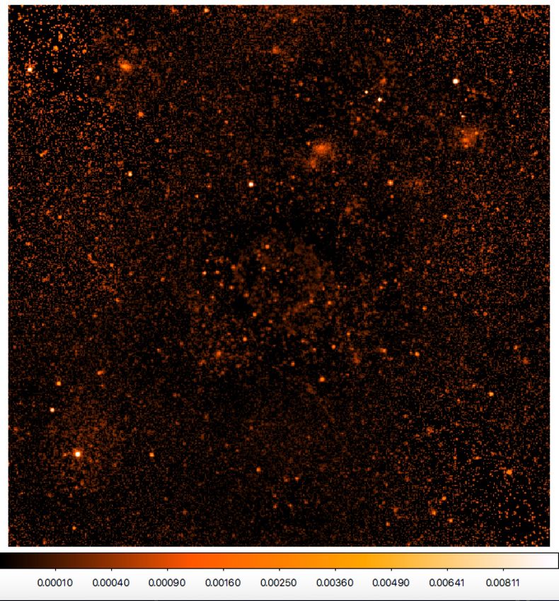
G. Hasinger et al.: ROSAT NEP Raster survey

Fig. 1. Raw hard-band (0.5−2 keV) image of the NEP raster scan (upper left, scale in raw counts); exposure map (upper right, scale in seconds);
exposure-corrected image (lower left, scale in counts s−1 ); count rate sensitivity map (lower right, scale in counts s−1 ). The image size is 6.4◦ ×6.4◦ ,
centred on the NEP. The pixel size is 4500 .

All the individual detections are consistent with the average sur-             varies from NH = 2.5 × 10²⁰ to 8.3 × 1020 cm−2 with a median of
vey image and the Gaia reference frame, so that we did not need                4.1 × 1020 cm−2 (Elvis et al. 1994). In the hard band this leads to
to apply an astrometric correction to the survey data.                         negligible absorption differences, while in the soft (0.1−0.4 keV)
                                                                               band the variation in transmission would be a factor of 7 across
3. X-ray analysis                                                              the field.
                                                                                    We accumulated an image in the 0.5−2 keV band centred on
3.1. Source detection
                                                                               the NEP with 512 × 512 pixels of 4500 each. Figure 1 (upper left)
We have restricted the basic source detection to the standard                  shows the resulting raw counts image, where the different expo-
hard ROSAT PSPC energy band (0.5−2 keV), corresponding                         sure times are clearly visible. The image in the upper right of
to PSPC PHA channels 52−201. For extragalactic work this is                    the figure shows the exposure map, calculated from the ROSAT
the most sensitive band, least affected by interstellar absorption             attitude files and the PSPC modified instrument map (MOIMP)
and also with the best PSPC angular resolution. The interstel-                 representing the detailed geometry of the PSPC support window
lar neutral hydrogen column density in our region of interest                  and the telescope vignetting. Some of the deeper pointings have

                                                                                                                                       A95, page 3 of 22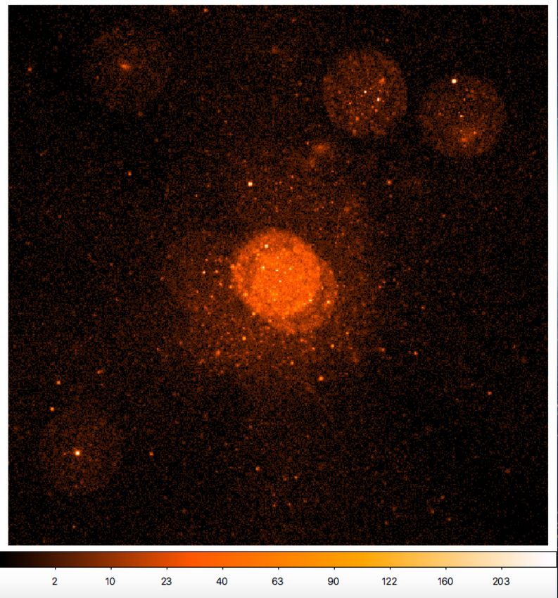
A&A 645, A95 (2021)

been carried out in a static (i.e. non-wobbled) observing mode.     of interest that were missed by the algorithms, which are flagged
For these, the structure of the PSPC support window is clearly      in the final catalogue.
visible in the exposure map, while it is partly smeared out in
the wobbled exposures. The detailed effect of the PSPC support      3.2. The ROSAT NEP Raster Catalogue
structure and the Wobble-Mode on the ROSAT deep surveys has
been discussed in Hasinger & Zamorani (2000). The image on          The third and last detection step uses a ML algorithm
the lower left is the exposure-corrected count rate map. Apart      (Cruddace et al. 1988; Boese & Doebereiner 2001) applied to
from some enhanced noise artefacts due to the relatively low        unbinned individual photons to both detect the sources and mea-
exposure in the upper left and lower right corners, the image       sure their final parameters. X-ray events in a circle of 30 radius
appears quite homogeneous, despite the large variations in expo-    around every entry in the regions of interest list were selected.
sure time, confirming the quality of the exposure map. Some         For a subset of 34 significantly extended sources (flagged in
bright diffuse X-ray sources can be readily identified.             the final catalogue) we increased the event selection radius to
    For the source detection we followed the RASS procedure         60 . The ML fit takes into account each photon with the appro-
described in Voges et al. (1999) and H06. However, we apply         priate PSF corresponding to the off-axis angle and energy at
the detection only to the hard-band image, and use the SEx-         which it was detected. An effectively smaller extraction radius
tractor (Bertin & Arnouts 1996) detection technique instead of      and therefore higher weight is given to photons detected near
the standard map detection method MDETECT before the final          the centre of the field, compared to those at the outskirts with a
maximum likelihood (ML) source characterization. The first step     worse PSF. The ML analysis yields a number of parameters for
is the local detection algorithm LDETECT, using a 3 × 3 pixel       each source. Most important is the source existence likelihood
detect cell, and a local measurement of the background in the       Lexi = − ln(P0 ), where P0 is the probability that the source count
surrounding 16 pixels. After a first pass at full resolution, the   rate is zero (see Boese & Doebereiner 2001). The threshold for
detect cell and corresponding background area are successively      this parameter has been set to Lexi ≥ 11 to define the final content
doubled in several more passes in order to also detect larger       of our survey. The likelihood analysis also determines the best
extended sources. The LDETECT step is applied to the raw            parameters for the source position and a corresponding position
image (see Fig. 1, upper left panel) uncorrected for exposure       error, the net detected counts of the source and its error, and an
time.                                                               estimate of the angular extent of the source and the likelihood
    A more elaborate background map is used for the next detec-     that it is extended. To estimate this extent the ML algorithm fits
tion step. Around every X-ray source detected by LDETECT            a Gaussian model added in quadrature to the PSF.
(using a higher likelihood threshold of L ≥ 10) a circular region        Table 1 gives the final catalogue of 805 detected X-ray
with a radius about the size of the detect cell is cut out from     sources in an abbreviated form; the complete catalogue is avail-
the raw image (the ‘swiss cheese map’). The remaining image is      able at the CDS. For all sources the parameters of the ML
then divided by the exposure map and binned into coarser pix-       analysis are quoted. A threshold of Lexi ≥ 11 has been applied
els. This cleaned, exposure-corrected image is fit by a smooth      throughout (see below). For a true estimate of source extent, a
two-dimensional spline. After the spline fit, a 4σ cut is applied   combination of existence likelihood and extent likelihood have
to pixels with count rates above the determined background in       to be considered (see discussion below). In order to convert the
order to remove artefacts from large diffuse sources and bright     source count rates to fluxes, following previous work, we assume
source haloes. This procedure is repeated until no more excess      an extragalactic point source with a photon index of −2 and
coarse pixels are found. Finally, a background map is produced      an interstellar column density of NH = 4.1 × 1020 cm−2 , folded
by applying the spline parameters to all pixels in the original     through the PSPC response matrix. A source with a 0.5−2 keV
image and multiplying by the exposure map. Figure 1 (lower          flux of 10−11 erg cm−2 s−1 yields a PSPC count rate of 0.815 cts s−1
right) shows the count rate sensitivity map, which is a combina-    in the 0.5−2 keV band. Because we restrict the source detection to
tion of the background map and the exposure map (see below).        the hard band, variations of NH across the field can be neglected.
    The standard second stage of the source detection using the     Therefore, the extragalactic point source fluxes can be readily con-
map detection algorithm MDETECT on the raw image with               verted into other spectral model fluxes. For 34 sources signifi-
the same detection cells as LDETECT, but taking the back-           cantly extended in the first ML analysis or by visual inspection, the
ground map estimate instead of the local background, turned out     extent characterization of the ML algorithm may be insufficient
not to be appropriate for our complex set of observations. The      because of the limited photon extraction radius, among other rea-
standard LDETECT and MDETECT algorithms are not able to             sons, and therefore the detected count rate could be significantly
accurately model the high-sensitivity confusion-limited areas in    underestimated. For these sources we determined the ML param-
the image, and the large exposure gradients and diffuse emis-       eters by doubling the event extraction radius; they are flagged
sion features produce a number of artefacts creating difficulties   with (1) in Col. (11) of the catalogue. Another ten non-extended
for the standard detection procedures. We therefore decided to      sources, which were originally not included in the source region
apply the SExtractor algorithm, well known in optical astronomy     of interest list, were manually fed through the normal ML detec-
(Bertin & Arnouts 1996), as the interim detection step offering     tion procedure and are also flagged in Col. (11).
possible regions of interest to the final ML source detection and        As a final quality check of the source detection we compared
characterization. This procedure works reasonably well for iso-     our catalogue to previous X-ray information in the HEROES
lated point sources, and even moderately confused sources, and      field, predominantly with the second ROSAT all-sky survey
for bright diffuse sources. However, it breaks down at the low-     (2RXS) source catalogue (Boller et al. 2016) and the second
exposure regions; in this case Gaussian statistics are no longer    XMM-Newton Slew Survey2 (XMMSL2) (see also Salvato et al.
appropriate and have to be replaced by Poissonian estimates.        2018), and with the fourth-generation XMM-Newton serendipi-
This is the reason, why we performed a detailed visual inspec-      tous source catalogue (4XMM-DR9, Webb et al. 2020). A total
tion and screening of the SExtractor source list selecting 1200     of 477 of our 805 X-ray sources have counterparts in the
regions of interest to be finally offered to the ML procedure. In
                                                                    2
this step we also manually inserted a number of source regions          https://www.cosmos.esa.int/web/xmm-newton/xmmsl2-ug

A95, page 4 of 22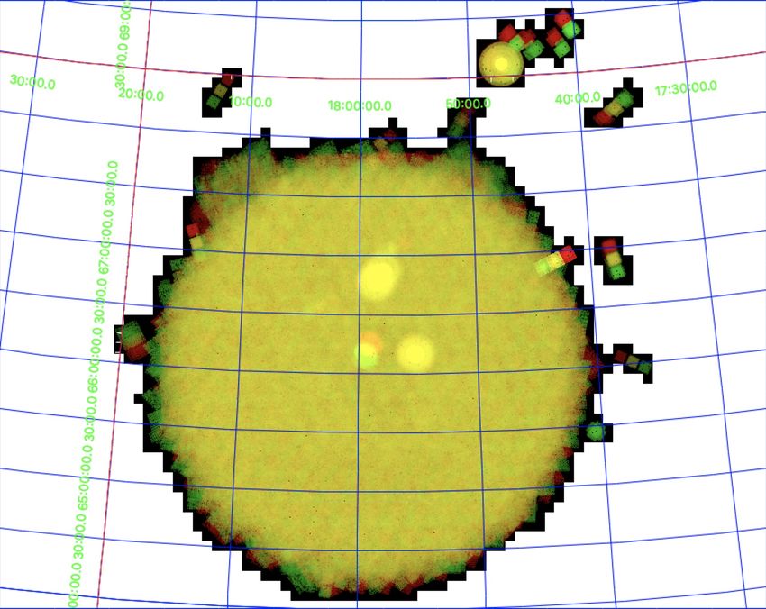
G. Hasinger et al.: ROSAT NEP Raster survey

Table 1. ROSAT NEP Raster X-ray Catalogue.

           (1)      (2)                (3)                 (4)        (5)      (6)       (7)       (8)         (9)             (10)      (11)
           XID      RAX                DecX                Err       Lexi     CTS      eCTS       Lext    Exposure      FX (0.5−2)        m
                    J2000              J2000               [00 ]                                               [s]      [10−14 cgs]
           1        261.4722856        68.15910084         9.9      13.3       8.2        3.1      0.0         1803             5.42
           2        261.7538598        69.44866306        11.0      30.5      12.3        3.6      0.0         1341            11.00
           3        261.9778949        67.81116425        14.1      29.1      16.9        4.3      9.0         2261             8.92
           4        262.1400312        67.54254828         9.8      21.1      14.4        4.2      0.7         2270             7.60
           5        262.4181202        68.79506796         9.2      26.9      14.4        4.0      0.0         1448            11.91
           6        262.4862510        66.86526820        11.5      12.2       8.9        3.4      0.0         1741             6.10
           7        262.5572915        65.73547731         9.5      17.4      10.8        3.6      0.0         3546             3.65
           8        262.5800581        68.16710175         8.5      17.3       8.6        3.1      0.0         1839             5.62
           9        262.9844661        65.37719281        13.5      19.3      14.0        4.1      0.0         3379             4.95
           10       263.0151617        67.80792566         9.7      13.6       9.8        3.5      0.1         2370             4.95
           ...
           796      277.4381113        67.81986356         5.4      68.4      25.3       5.3      0.0          1637           18.49        1
           797      277.4522820        64.58551610         8.4      24.8      18.5       4.8      0.2          4657            4.75
           798      277.5094136        66.75661056         6.0      53.0      22.9       5.0      0.0          2095           13.04
           799      278.0683716        68.54311384         9.8      21.1      10.5       3.5      0.1          1091           11.55        1
           800      278.1405809        68.61500503         8.1      42.7      17.1       4.2      0.1          1044           19.62
           801      278.1552805        68.80281717         6.9     364.3     127.9      11.5     58.1           783          195.44        1
           802      278.1773278        69.07251242        13.6      14.7       6.3       2.7      0.0           438           17.22
           803      278.4506109        69.36011661        13.7      18.7       9.8       3.3      0.0           323           36.12
           804      278.6549948        69.52945061        11.7     155.2      14.9       3.8     10.9           320           55.50
           805      278.6965904        69.41463855        23.1      46.9       5.0       2.2      0.9           306           19.50
Notes. Columns: (1) internal XID identification; (2) and (3) X-ray source coordinates in J2000.0; (4) position error (including systematics); (5)
existence likelihood Lexi ; (6) and (7) detected number of net counts and statistical error; (8) extent likelihood Lext (see text for discussion of actual
extent determination); (9) exposure time; (10) 0.5−2 keV source fluxes in units of 10−14 erg cm−2 s−1 ; (11) flag for manual ML input. The full table
is available at the CDS.

literature. In particular there are 431 matches with 2RXS,                    than one spurious source in the overall survey. This threshold is
83 with 4XMM-DR9, and 40 with XMMSL2. About half of                           more conservative than the limits of Lexi ≥ 6.5 or Lexi ≥ 9, for
these matches (228) are also present in the H06 catalogue. As                 example, selected for the 2RXS source catalogue (Boller et al.
expected, the 2RXS analysis has a greater difficulty in deter-                2016), which lead to a much larger spurious source fraction
mining source extents and resolving confusion, but yields bet-                of about 30% and 5%, respectively. The treatment is, however,
ter accuracy for isolated sources in the outskirts of our survey.             rather simplified. In reality, systematic effects can increase the
As we discuss below, the literature data (in particular the bet-              number of spurious sources (e.g., the high diffuse surface bright-
ter XMM-Newton positions) confirmed almost all of our optical                 ness around bright extended and point sources discussed above)
counterparts in the overlapping areas, except for 17 cases iden-              and the effects of confusion. Using the likelihood threshold of
tified as high-quality optical counterparts that would have been              Lexi ≥ 11, we can thus expect a handful of spurious sources,
missed in our analysis.                                                       consistent with the optical identifications discussed in Sect. 4.4.
                                                                              Together with a careful manual screening of spurious sources
                                                                              and merging of split source components, we arrive at a cata-
3.3. Sensitivity limits
                                                                              logue of 805 X-ray sources (see Table 1). A total of 254 of our
An important consideration is the setting of the source detec-                sources match entries in the H06 catalogue within 2.5σ error cir-
tion threshold Lexi and thus the corresponding sensitivity func-              cles. These matches are indicated with black solid circles in the
tion for the survey. It has to be chosen to maximize the number               relevant figures throughout this paper. The classical confusion
of true sources in the survey, and to minimize the number of                  limit in radio astronomy is defined as 40 beams (i.e. statistically
spurious sources. The expected number of spurious sources is                  independent detection cells) per source (Condon 1974). With the
the above probability P0 multiplied with the number of statisti-              number of independent trials estimated above, this corresponds
cally independent trials ntrial across the field. Given the rather            to 1145 sources in the whole survey, or about 28 sources deg−2 .
complex setup of our survey, and the intricacies of the ML                    Our average source density is below this number, but in the deep-
source detection algorithm, it is not possible to determine ntrial            est pointed areas around the NEP the source density is higher
analytically. A rough estimate is the number of statistically                 than this classical confusion limit.
independent detection cells in the LDETECT process, which is                       In order to use the survey for quantitative statistics, it is
(512 × 512)/(3 × 3) = 29127. Below, in the context of calculating             important to calculate a survey selection function. This is equiv-
the survey sensitivity function, we derive the average effective              alent to the sky coverage solid angle, within which sources of
extraction radius for our ML analysis, which is 1.35 pixels, or               a particular brightness would have been detected in the sur-
60.800 . Using this number for the size of the detection cell, we             vey. For the ML algorithm described above, with its intricacy
arrive at 45785 independent trials. Therefore, an existence like-             of different effective detection cell radii for individual photons,
lihood threshold of Lexi ≥ 11 is applied to statistically obtain less         it is not possible to calculate a sensitivity limit analytically.

                                                                                                                                       A95, page 5 of 22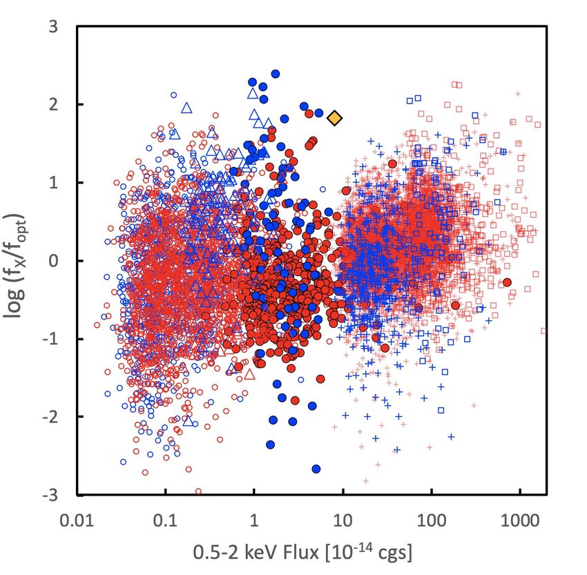
A&A 645, A95 (2021)

Fig. 2. Left: ROSAT NEP Raster Survey sensitivity function (red) compared with the RASS NEP survey of H06 (blue). Right: characterization
of extended sources in the diagram of existence vs. extent likelihood. Red circles correspond to AGN1, blue circles to AGN2, pink circles to
normal galaxies, green squares to clusters of galaxies, and yellow asterisks to stars. Black circles around the symbols indicate sources from the
H06 catalogue. This figure, and the corresponding following figures, are only shown for the unique optical counterparts (see Sect. 4.4). Bright
point sources (AGN, stars) appear to be extended because of the imperfect description of the PSF in the ML algorithm. The dashed line shows an
empirical separation between true and spurious extension.

Therefore, some publications resort to extensive Monte Carlo              at the count rate sensitivity map shown in Fig. 1 in the lower right
simulations for the determination of the sky coverage func-               panel.
tion (see e.g., Cappelluti et al. 2009). For the statistical appli-            To convert this map into proper source fluxes we have to
cations in this paper it is appropriate to approximate the                sum the count rate sensitivity distribution over all pixels in the
sensitivity map by a simple signal-to-noise ratio calculation,            512 × 512 pixel images to obtain the corresponding cumulative
following the procedure described in H06. In the case of sig-             area in units of deg2 , and to divide the count rates by the PSF
nificant background in the detection cell the likelihood can be           correction factor of 0.77 and by the above count rate to flux con-
approximated by a Gaussian probability distribution. A detec-             version factor of 8.15 × 10¹⁰ cts erg−1 cm2 . This way we arrive at
tion likelihood of Lexi ≥ 11 almost exactly corresponds to a              the final survey selection function shown in red in Fig. 2 (left) in
Gaussian probability of 3σ, so we base our sensitivity calcula-           comparison to the corresponding curve of H06 (using their tabu-
tion on this limit. In the background limited case, √ the signal-         lated values for extragalactic point sources). The total solid angle
to-noise ratio can be calculated as S /N = S / S + B, where               covered in our survey at high fluxes is 40.9 deg2 , about half that
S is the net detected counts of a source, and B is the number             of H06; however, our survey is about 0.5 dex deeper than H06.
of background counts in the source detection cell. For a given
background brightness per pixel of b, the background counts in            3.4. Extended source analysis
a circular detect cell of radius rb is simply B = bπrb2 . For the pur-
pose of this analysis b is assumed error-free because it has been         The ML algorithm is very useful for the separation between point
determined from a large background map with high statistical              sources and clusters. It weights different photons according to
accuracy.                                                                 the size of their individual PSF model, and therefore is arguably
    Compared to the original extraction radius of 30 for the ML           the most sensitive method for detecting extended sources in a
algorithm, the effective extraction radius applicable for the back-       photon-starved situation, where the extent is not much larger
ground calculation is smaller, because every photon is treated            than the PSF. However, because of the necessary approxima-
with its own PSF. The task at hand is now to determine the effec-         tions in the description of the actual PSF, which depends on
tive background cell radius rb , which is equivalent to the ML            the off-axis angle and energy and also has extended scattering
treatment in our survey. For this purpose, we chose 71 X-ray              wings, the method tends to detect spurious extents in bright
sources detected with likelihoods of 10 ≤ Lexi ≤ 12 and varied            X-ray point sources. This is shown in Fig. 2 (right), where the
the background cell radius rb until the distribution of signal-to-        extent likelihood is compared to the existence likelihood for the
noise ratios determined by the ML procedure agreed with that of           whole X-ray catalogue. Most clusters from the H06 catalogue
the Gaussian calculation. This calibration results in an effective        are clearly segregated from the rest of the sample, with extent
background cell radius of rb = 1.35 pixels = 60.800 . The survey-         likelihoods Lext ≥ 4−5. However, above existence likelihoods of
integrated PSF determined above contains 77% of the flux within           Lexi ≥ 50 the bright point sources (yellow stars and red AGN1
this radius. Multiplying the background cell area with this radius        from H06) are creeping into the significantly extended area. We
to the background map derived above, applying the above S/N               therefore empirically determined the dashed line to discriminate
calculation formula, and dividing by the exposure map, we arrive          truly extended sources. There is one star from H06 (#3970),

A95, page 6 of 22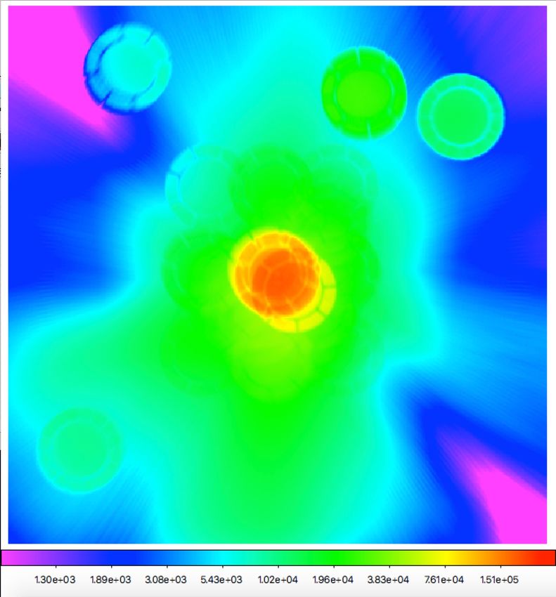
G. Hasinger et al.: ROSAT NEP Raster survey
which appears significantly extended with an extent likelihood
Lext = 12.4. There are actually two bright stars in the same error
circle, so that the extent could be due to the double star nature.
An additional complexity occurs in the case of AGN residing in
clusters of galaxies, which may show X-ray extent despite being
identified with a point source. The most interesting case is the
AGN1 #5340 in the H06 catalogue, the object in the top right
corner of Fig. 2 (right). This is the well-known bright HEAO-1
catalogue source H1821+643 (Pravdo & Marshall 1984) inside
the massive cluster ClG 1821+64 (Schneider et al. 1992), later
also detected by Planck through its Sunyaev-Zeldovich effect
(Planck Collaboration XXIX 2014). An extended X-ray source
superposed on the AGN point source extent has been indepen-
dently measured for this object with the ROSAT HRI (Hall et al.
1997); therefore, the extent measured in our analysis is approx-
imately correct and thus the dashed line maybe a bit too
conservative.
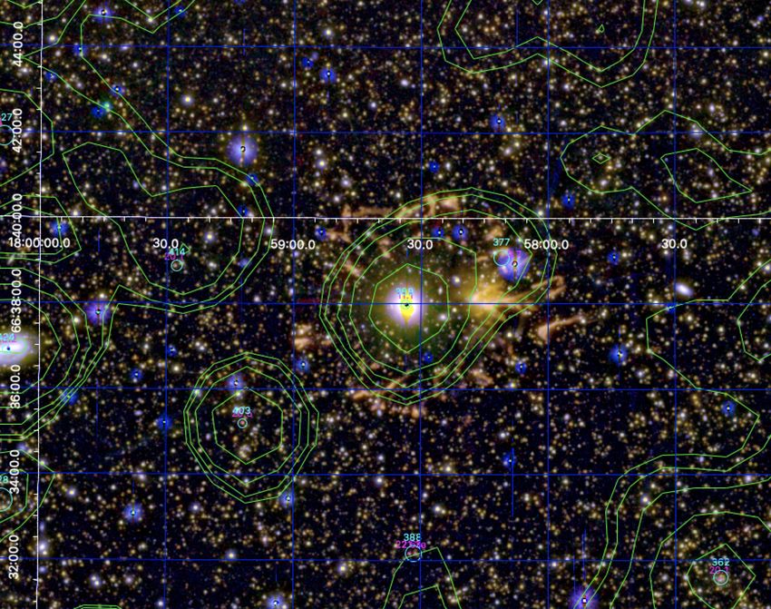
4. Multi-band observations Fig. 3. False colour HEROES image of the shell around the planetary
nebula NGC 6543 (Cat’s Eye Nebula) close to the NEP. Blue repre-
4.1. HEROES optical/NIR wide-field imaging sents the HSC g-band image and predominantly shows the green [OIII]
line. Green represents the HSC r-band and predominantly shows Hα.
The ultimate goal of HEROES (see e.g., Songaila et al. 2018) Red corresponds to the 4.5 µm Spitzer image and mainly shows dust
is to cover an area of 120 deg2 around the NEP, where emission.
the eROSITA X-ray all-sky survey (Merloni et al. 2012;
Predehl et al. 2021) will have some of its deepest coverage.
This survey utilizes the wide-field capability of the Hyper from the median. Co-adding the images to a certain degree also
Suprime-Cam instrument (HSC; Miyazaki et al. 2012) on the reduces non-astronomical artefacts like the reflection ‘ghosts’
Subaru 8.2 m telescope, as well as the MegaPrime/MegaCam from bright stars outside the FOV. Faint sources are detected
and WIRCam instruments on the 3.6 m CFHT to map this large by forced photometry running simultaneously across all filters
area. HEROES comprises grizy broad-band images with limit- (Magnier et al. 2020b). If a source is detected with more than
ing magnitudes around 26.5−24.5 and NB816 & NB921 narrow- 5σ in any particular band, photometry is forced on all other
band images with limiting magnitudes around 24 from Subaru, bands. This allows us to calculate photometric redshifts for a
as well as U- and J-band images with limiting magnitudes 25.5 large fraction of all sources. Whenever available, we used Kron
and 22.1, respectively, from CFHT. So far an area of approx- magnitudes for this purpose. For each band we also obtain a
imately 40 deg2 has been covered with HSC during 2016 July star–galaxy separation parameter. The original HSC catalogue of
1−10 and 2017 June 21−28 while the CFHT data were taken objects detected significantly in at least one band contains 23.9
from 2016 March 18 to 2016 August 20. The HSC observations million objects. However, caution is required to avoid false posi-
were acquired in a closely packed set of dithered observations tive detections because a single artefact in any band will produce
described in detail in Songaila et al. (2018). an entry in the catalogue. Therefore, we have selected objects
A formal publication of the HEROES catalogue is in prepa- detected in at least two bands for the photometric redshift deter-
ration. Here we give some basic information about our data mination described below.
reduction process. Rather than using the HSC standard pipeline, The CFHT WIRCAM J-band data was reduced and stacked
which at the time of the massive data reduction task was not with a custom version of the AstrOmatic image analysis system
yet available to us, we analysed all HSC images with the Pan- (Bertin et al. 2012), in particular using the packages SCAMP,
STARRS Image Processing Pipeline (IPP; Magnier et al. 2020a), SWarp, MissFITS, and SExtractor (Bertin & Arnouts 1996).
which was well tested and available on a dedicated computer The CFHT MegaCam U-band data were reduced and stacked
cluster allowing fast processing of the large data volume. The with the excellent MegaPipe imaging pipeline at the Canadian
IPP pipeline can be adapted to any wide-field imaging dataset, Astronomy Data Center (courtesy Stephen Gwyn). The astro-
as long as the instrument calibration characteristics are incor- metric calibration was done with Gaia, and the photometric
porated. For HSC this required mainly the accurate description calibration with a combination of SDSS data and a nightly
of the significant differential image distortion across the large zero-point calibration from MegaCam on photometric nights.
FOV. The details of the Pan-STARRS Pixel Processing (i.e. the This photometric calibration was bootstrapped to the few non-
detrending, warping, and stacking of the images) are described photometric nights so that the zero-point calibration is self-
in Waters et al. (2020). Each exposure is cleaned from instru- consistent to 0.015 mag. Again, we used the Kron magnitudes
mental effects, and photometry and astrometry are performed by for the subsequent analysis.
comparing the objects detected on the individual images with An example of the excellent HEROES image quality, and
the Pan-STARRS reference catalogue. This process also yields also the various artefacts produced by bright objects in the field,
the individual image quality in terms of seeing and photomet- is given in Fig. 3 showing the shell around the planetary neb-
ric transmission. The seeing was typically very good during ula NGC 6543 (Cat’s Eye Nebula) that was ejected by its pre-
the observations, with a median around 0.700 and a large frac- decessor red giant star. The actual PN in the centre of the
tion of photometric transparency. For stacking the images into image is completely over-exposed. The high density of faint
a common pixel grid we selected exposures with seeing better background objects shows the excellent sensitivity of the data.
than 1.3600 and photometric zero points not fainter than 0.3 mag The NEP lies at relatively low Galactic latitudes, and therefore
A95, page 7 of 22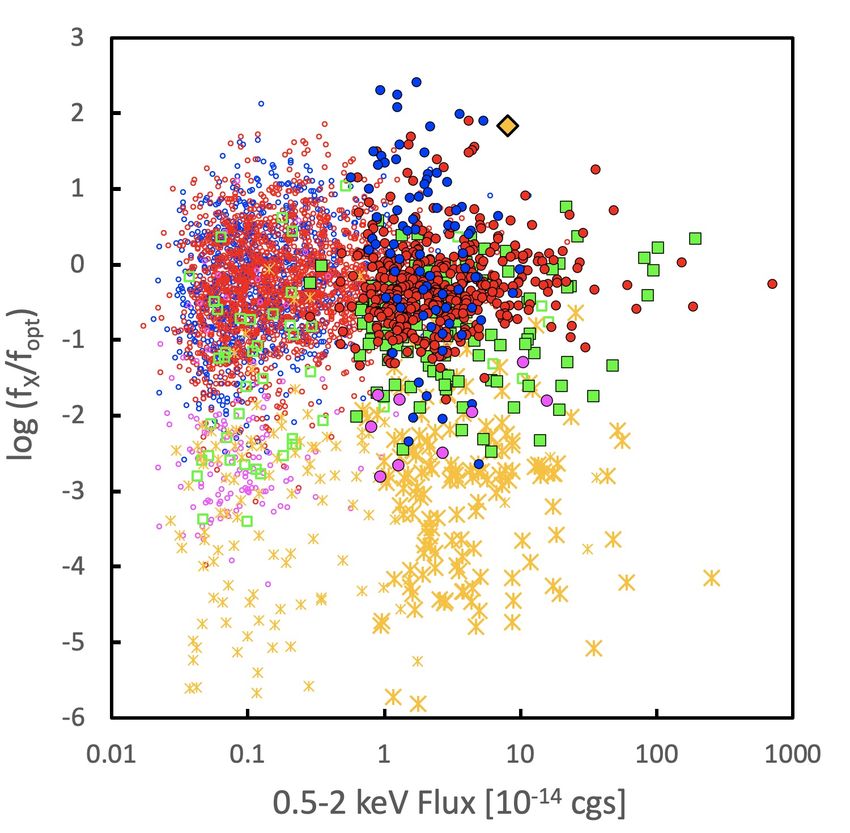
A&A 645, A95 (2021)

Fig. 4. Left: map of the Spitzer IRAC 3.6 µm (green) and 4.5 µm (red) coverage in the Spitzer Cosmic Dawn Survey around the NEP (Moneti
et al., in prep.). Right: comparison between spectroscopic and photometric redshifts in our sample. Green circles are 541 ‘clean’ galaxies with
spectroscopic redshifts in the HEROES field. Black dots are a sample of 263 AGN with spectroscopic redshifts in the field. The dashed and dotted
lines refer to a redshift error of ∆z/(1 + z) = ±0.15.

contains a rather large number of overexposed foreground stars           areas of the sky, covering a total of 40 deg2 . These three fields
showing up in this image (in cyan). In order to obtain reli-             were carefully selected to contain a minimum of bright stars,
able optical photometry for brighter objects, which are satu-            and low dust emission and zodiacal light. In addition, these
rated in the HEROES HSC images, we also made use of the                  fields already have substantial multi-wavelength coverage, and
SDSS DR16 (Ahumada et al. 2020), the Pan-STARRS DR1 &                    will be observed with other space observatories, enabling us to
DR2 (Chambers et al. 2016), and Gaia DR2 (Gaia Collaboration             perform a large amount of ancillary science. One of these fields
2018) catalogues. We also cross-correlated our samples with              encompasses an area of 10 deg2 around the NEP, in the middle of
the far-UV and near-UV photometry from the GALEX surveys                 the HEROES field. The NASA Spitzer telescope has performed
(Martin et al. 2005).                                                    a large survey (P.I. P. Capak) of two Euclid Deep Fields, the
                                                                         Euclid/WFIRST Spitzer Legacy Survey (Capak et al. 2016). A
                                                                         total of 5286 h of Spitzer observing time are distributed over
4.2. Mid-infrared observations of the HEROES field
                                                                         20 deg2 split between the Chandra Deep Field South and the
For photometric information in the 3−25 µm band across the               NEP, with an exposure time of 2 h per pixel. The primary goal
whole HEROES field we used the WISE all-sky survey cat-                  is to enable definitive studies of reionization, z > 7 galaxy for-
alogues. For the shorter wavelength W1 (3.4 µm) and W2                   mation, and the first massive black holes. The data will also
(4.6 µm) bands we used the CatWISE2020 all-sky catalogue                 enhance the cosmological constraints provided by Euclid and
(Eisenhardt et al. 2020) (see also Marocco et al., in prep.),            Nancy Grace Roman Space Telescope (WFIRST). We are using
containing about 1.89 billion objects observed by the Wide-              a preliminary Spitzer data product. The final survey is being pre-
field Infrared Survey Explorer (WISE and NEOWISE), both of               pared for publication as part of the Spitzer Cosmic Dawn Sur-
which have higher sensitivity and higher angular resolution than         vey (Moneti et al., in prep.), covering the three Euclid deep
the original ALLWISE catalogue (Cutri et al. 2013). The Cat-             fields and several other Euclid calibration fields. These authors
WISE2020 catalogue in the HEROES field contains 2.4 million              developed a new IRAC data processing pipeline and used the
objects and gives fluxes in the W1 and W2 band, which we                 availability of highly precise astrometry available from Gaia to
converted to the AB magnitude system. For the longer wave-               reprocess nearly all available Spitzer data in this field (exclud-
length W3 (12 µm) and W4 (22 µm) bands we used the original              ing short observations like calibrations on bright stars), which
ALLWISE catalogue (Cutri et al. 2013), again converting to AB            will be essential for the Euclid calibration and for high-redshift
magnitudes. At the faintest magnitudes the CatWISE2020 and               legacy science. Figure 4 (left) shows the sky coverage of the two
ALLWISE catalogues are, however, severely confusion limited.             channels 3.6 µm (I1) and 4.5 µm (I2) with the widest deep cover-
In the centre of the HEROES field, we therefore also made use of         age of the NEP. We used SExtractor (Bertin & Arnouts 1996) to
the Spitzer Observations of the Euclid Deep Field North (Moneti          extract source positions and magnitudes from the IRAC images
et al., in prep.).                                                       in these two bands, yielding a catalogue of almost one million
     The ESA Euclid mission is making great progress towards             sources.
its launch, scheduled in 2022. Euclid’s main goal is to survey
a large fraction of the sky and image billions of galaxies to            4.3. Photometric redshifts
investigate dark energy and dark matter over the history of the
Universe. Roughly 10% of the observing time will be dedicated            Based on the grizy HSC detections, we joined the GALEX,
to the Euclid Deep Fields, repeatedly observing three specific           MegaCam, HSC, WIRCAM, SDSS, Pan-STARRS (partially),

A95, page 8 of 22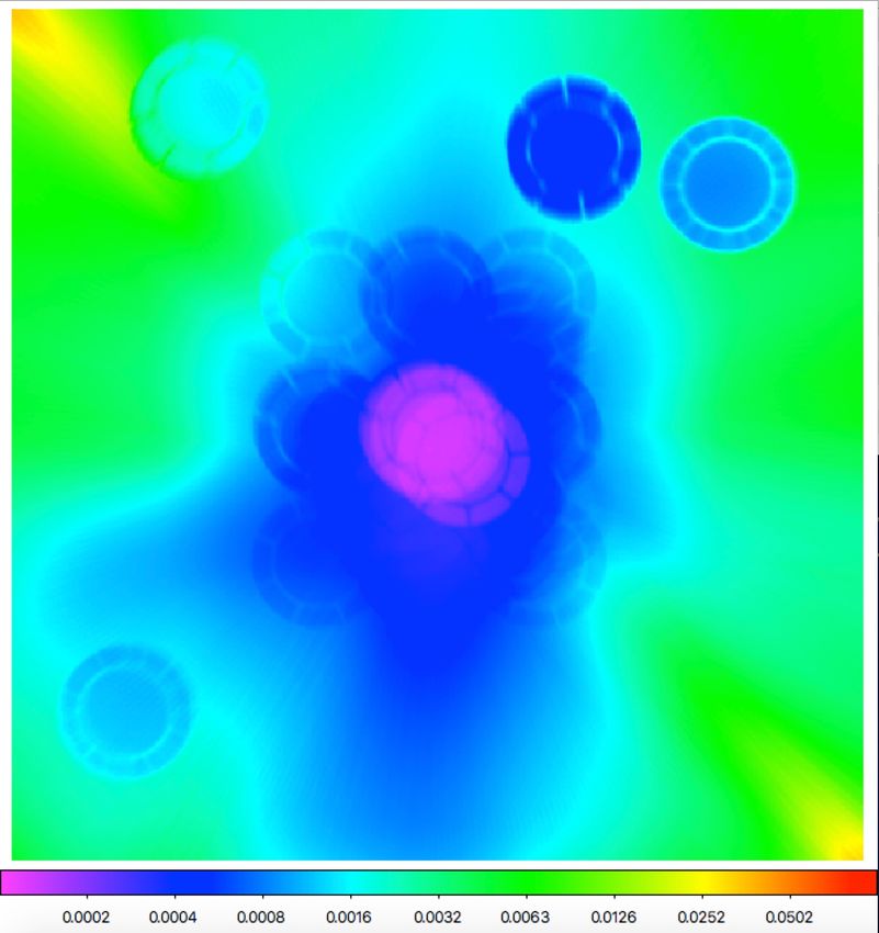
G. Hasinger et al.: ROSAT NEP Raster survey

Fig. 5. Some high-quality examples of photometric redshift fits to X-ray counterparts, illustrating different AGN SED models. The MRK231 and
TORUS spectra have the largest mid-IR fraction of all chosen models.

CatWISE2020, ALLWISE, and Spitzer IRAC catalogues into a               W3 & W4 mid-IR bands, we had to extrapolate some of the
single source list by association through positional matching. For     Ananna et al. (2017) hybrid galaxy and QSO SEDs to longer
the UV, optical, and NIR images and for the IRAC catalogue we          wavelengths. Our AGN photometry also required us to include
allowed a maximum distance of 100 , while for GALEX and WISE           the heavily absorbed TORUS model SED from Polletta et al.
we allowed a maximum of 300 . This way we obtained a combi-            (2007). We adopted the Small Magellanic Cloud extinction law
nation of a maximum of 22 photometric bands (GALEX FUV                 from Prevot et al. (1984) (see Salvato et al. 2009) to allow for
& NUV, HEROES UgrizyJ plus NB816 & NB921, SDSS ugriz,                  intrinsic reddening of the sources, exploring E(B − V) values
as well as CatWISE2020 W1 & W2, ALLWISE W3 & W4, and                   from 0 to 0.35 in steps of 0.05. Before the final fit we made slight
IRAC I1 & I2 bands). Ideally, for the highest accuracy of photo-       adjustments to the zero points for each band, using the LePhare
metric redshifts, the forced aperture photometry should be used        self-calibration procedure with 541 spectroscopic redshifts for
in all bands. However, this is not possible in the case of a com-      clean galaxies (i.e. no AGN contribution, not confused, inter-
bination with catalogues from the literature. In some cases of         mediate magnitudes) and 263 AGN with spectroscopic redshifts
very faint optical counterparts or objects confused with brighter      observed by HEROES in the field.
nearby sources, we determined the correct magnitudes through               Figure 5 shows four high-quality examples of photomet-
manual aperture photometry.                                            ric redshift fits for X-ray detected AGN candidates, illustrating
    A nice review of the application of photometric redshift tech-     different spectral energy distributions. The MRK231 and TORUS
niques in modern wide-field surveys is given by Salvato et al.         SEDs have the largest relative mid-IR contributions, and sizeable
(2019). We determined photometric redshifts using the LeP-             number of X-ray counterparts (16 and 5, respectively), and even
hare code (Arnouts et al. 1999; Ilbert et al. 2006). We followed       more mid-IR selected AGN (54 and 26, respectively) require
the procedure described in Ilbert et al. (2009), basically fitting     these models. They are reminiscent of the Spitzer power law
three different model families (galaxies, AGN, and stars) to the       AGN SEDs detected in the Chandra deep fields (Donley et al.
spectral energy distribution. For the galaxy SED templates we          2007). The TORUS SED model from Polletta et al. (2007) is
used the models from Laigle et al. (2016), including emission          an addition compared to the work of Salvato et al. (2009) and
lines. For AGN we applied the specific modifications described         Ananna et al. (2017).
in Salvato et al. (2009), wherever possible correcting for time            We checked the quality of the photometric redshifts using
variability between the SDSS and HEROES data, and taking               the 541 reference galaxies (see the green circles in Fig. 4, right).
the different SED templates used for point-like and extended           The fraction of catastrophic outliers with |∆z|/(1 + z) ≥ 0.15
AGN in Ananna et al. (2017). Because we include the WISE               is only 4.6%, and the rms error of all galaxy photometric

                                                                                                                          A95, page 9 of 22
A&A 645, A95 (2021)

redshifts is h|∆z|/(1 + z)i = 0.033. The accuracy of the galaxy
photometric redshifts is thus quite comparable to other sur-
veys using broad-band photometry, but somewhat worse than
e.g., those in the COSMOS field (Ilbert et al. 2009; Salvato et al.
2009; Laigle et al. 2016), mainly because COSMOS has a large
number of intermediate band filters and much deeper imaging.
We also compared the photometric and spectroscopic redshifts
for the reference sample of 263 AGN in the field (black dots in
Fig. 4, right panel). The fraction of catastrophic outliers is about
22%, and these are dominated by relatively bright AGN1. The
rms error of all AGN photometric redshifts is h|∆z|/(1 + z)i =
0.06. In about 4% of all cases there is a secondary maximum
in the photometric redshift probability distribution fitting bet-
ter to the spectroscopic redshift. This quality is very similar
to the results obtained by Ananna et al. (2017) for a sample of
similar quality. Broad-band photometric redshifts for AGN1 are
notoriously difficult for several reasons: their SEDs are prac-
tically power laws with superposed emission lines, which are
not prominent in broad photometric bands. Time variability or
photometric errors can cause spurious spectral features, which
the SED fit clings to. However, despite the potentially erro-
neous photometric redshifts, the classification as AGN is unique.
Therefore, our photometric redshifts are more than sufficient
for a crude optical identification and source classification of the    Fig. 6. Separation between X-ray and optical–NIR counterparts in arc-
X-ray counterparts.                                                    seconds of right ascension and declination. The symbols are the same
                                                                       as in Fig. 2 (right).
4.4. Optical identifications
The first step towards the optical identification of X-ray sources     15% of the stellar identifications may be incorrectly associated,
is the astrometric correction, which was already applied as part       likely due to the large density of stars in the field. Clusters,
of the data preparation in Sect. 2. Therefore, the final output        groups, and individual galaxies have an even wider distribution.
catalogue does not need further astrometric corrections. Opti-         This may be due to the fact that the X-ray emission is not always
cal identification is an iterative procedure, which in the case        centred on the brightest galaxy. We therefore use only AGN to
of relatively large error circles with multiple possible counter-      calibrate the identification procedure. The first step is the deter-
parts has a significant statistical uncertainty. The results there-    mination of possible systematic position errors in the dataset.
fore contain a probabilistic element, which is addressed below.        The ML X-ray detection algorithm gives the statistical position
The availability of the optical identification catalogue of H06,       error (see Table 1), which can be compared to the distribution
as well as the existence of a number of additional spectroscopic       of counterpart offsets. For this purpose, we selected a reference
redshifts from the literature, are important prerequisites for the     sample of 231 high-quality AGN identifications, consisting of
identification procedure. The NEP field is at a comparatively low      141 AGN from H06, 10 other AGN with spectroscopic redshifts
Galactic latitude (b ≈ 28◦ ), and therefore contains a large num-      from the literature, and 80 high-quality AGN identifications
ber of stars, many of which may also be faint X-ray sources.           selected from their mid-IR colours (with WISE W1−W2 > 0.8;
The optical position accuracy for bright stars is reduced, par-        see Assef et al. 2013). First, we calculate the cumulative distri-
tially because they are often saturated in the deep CCD images.        bution of position offsets in units of the 1σ statistical position
Wherever possible, therefore, we make use of the Gaia DR2 cat-         errors, which is shown as a grey line in Fig. 7 (right). This is
alogue (Gaia Collaboration 2018).                                      significantly wider than the Gaussian model expectation, shown
     Arguably the most important element of reliable identifica-       as black dashed curve. We then iteratively applied a system-
tions is the existence of the mid-IR catalogues from WISE and          atic position error in quadrature to the statistical errors, until we
Spitzer. As we show below, the identification procedure for the        found a reasonable match with the Gaussian expectation at a sys-
805 X-ray catalogue sources yields 766 high-likelihood optical         tematic error value of 300 . The corresponding cumulative distri-
candidates (identification quality IQ = 2), while in 39 cases          bution for our reference AGN sample is shown as the red curve.
there is an ambiguity with several possible counterparts (IQ =         We then applied the same systematic error to the remaining 301
1). There are 74 additional and possibly interesting objects in        AGN identifications in the sample. Their cumulative position
the error circles of high-likelihood counterparts, which are noted     offsets are shown as the blue line in Fig. 7 (right). We also tested
in the optical ID catalogue with IQ = 0. The following figures         the normalized offset distributions separately for AGN1 and type
only show the 766 high-likelihood (IQ = 2) counterparts.               2 AGN (AGN2) for both the reference sample and the remain-
     Figure 6 shows the offsets in right ascension and declination     ing AGN and did not find significant differences. The fact that
between the position of the X-ray source and that of the high-         all normalized offset distributions almost perfectly match the
likelihood optical counterpart. Figure 7 (left) shows the cumu-        Gaussian expectation for the reference sample, which is typically
lative distributions of position offsets (in arcseconds) for AGN       from brighter X-ray objects, and for the fainter remaining AGN,
(red); stars (yellow); and galaxies, clusters, and groups (green),     confirms the accuracy of the ML errors as well as the systematic
identified below. AGN show the narrowest distribution, with a          errors.
half-radius of 8.500 . Stars, on the other hand, have a somewhat           We now can correlate the whole sample both with the opti-
wider distribution (half-radius 9.800 ). This indicates that about     cal (HEROES) and the mid-IR (WISE, Spitzer) catalogues to
A95, page 10 of 22
G. Hasinger et al.: ROSAT NEP Raster survey
Fig. 7. Left: cumulative distribution of position offsets (in arcseconds) for different classes of sources. AGN have a narrow distribution with a
half-radius of 8.500 , while stars have a slightly wider distribution (9.800 ), indicating some possible misidentification among ∼15% of the stars.
Clusters and groups have an even wider distribution because the X-ray emission is not always centred on the brightest galaxy. Right: cumulative
distribution of position offsets in units of the 1σ position errors compared to a Gaussian model (black dashes). The grey line shows the distribution
for 231 high-quality reference AGN (see text) before the application of a systematic position error. The red line shows the same 231 reference
AGN after a systematic position error of 300 has been applied to each statistical error. The blue line shows the offset distribution for the remaining
301 AGN applying the same 300 systematic position error.
look at the number and magnitude distribution of the expected association becomes meaningless. We therefore have to intro-
counterparts in the X-ray error circles, both the real counterparts duce additional information and prior expectations into the iden-
and random field associations. We use a correlation radius of tification process. As discussed above, this is naturally a proba-
2.5σ around each of the 805 X-ray sources to obtain the cumula- bilistic approach and no longer yields unique identifications. In
tive iAB and W1 magnitude distributions of objects, respectively, principle there is the elaborate Bayesian multi-catalogue match-
shown by the green lines in Fig. 8. The blue lines show the mag- ing tool NWAY3 (Salvato et al. 2018), where several input cat-
nitude distribution of field objects within 805 randomly chosen alogues can be cross-matched and a number of priors can be
circles of the same 2.5σ radius. The dashed red lines show the introduced, which also calculates the likelihood for every pos-
difference between X-ray error circles and field circles (i.e. the sible positional coincidence. However, in the case of incomplete
expected cumulative magnitude distribution for all counterparts catalogue information, and in the presence of significant system-
associated with the X-ray sources). This gives the possibility of atic errors (e.g., non-astronomical false positive detections in the
having more than one physical association per error circle (e.g., optical catalogue) or the presence of source confusion both in the
pairs, groups or clusters of galaxies, merging AGN, or star clus- X-ray catalogue and in the CatWISE2020 catalogue it is very
ters). In making this subtraction one has to take care of the effect cumbersome to construct the appropriate prior for this method.
discussed in Brusa et al. (2007) and Naylor et al. (2013), namely Figure 9 gives a visual impression of the difficulty of optical
that the magnitude distribution of field galaxies around bright identification in the complicated situation of faint optical coun-
objects is significantly shallower than around faint objects, lead- terparts with relatively large error circles and possibly confused
ing to negative values in the subtraction. The dashed red lines settings. ROSAT X-ray contours are superimposed in a loga-
have therefore been calculated piece-wise in different magni- rithmic scale on a false-colour image with the Spitzer bands I2
tude intervals before constructing the cumulative distribution. (red) and I1 (green) and the HEROES i-band image (blue). This
The solid red lines show the actual magnitude distribution of 180 × 150 image is centred on the planetary nebula NGC 6543
the selected best optical counterparts in Table 3. For magnitudes close to the centre of the HEROES field (see also Fig. 3). The
19.5 the expected number centre of the image has two credible AGN counterparts. Given
of field objects per error circle increases above one, reaching these difficulties, we had to resort to the tedious task of visually
values of ∼20 and ∼6 at iAB = 25 and W1 = 22, respectively.
In this situation the optical identification purely by positional 3
https://github.com/JohannesBuchner/nway
A95, page 11 of 22A&A 645, A95 (2021)
Fig. 8. Cumulative magnitude distributions in circles with 2.5σ error radii around the 805 X-ray sources (green line), and the same number of
randomly chosen positions (blue line). The dashed red line shows the difference between source and random circles, while the thick red line shows
the actual magnitude distribution of the X-ray counterparts. Left: Subaru HSC i band. Right: CatWISE2020 W1 band. The dotted black line shows
the cumulative distribution of random mid-IR selected AGN candidates with W1−W2 > 0.8.
inspecting every individual error circle and manually selecting can be readily identified through their peculiar mid-IR colours
and characterizing the most likely optical counterpart, consider- (see e.g., Stern et al. 2012; Assef et al. 2013). We used the clas-
ing a number of prior expectations. Previously published deep sical criterion W1−W2 > 0.8 to identify mid-IR AGN candi-
X-ray surveys (e.g., Brandt & Hasinger 2005) show that the dates. The dotted black line in Fig. 8 (right) shows the randomly
largest fraction of X-ray sources at our flux limit are AGN, fol- expected number of mid-IR selected AGN per X-ray error cir-
lowed by stars, and clusters of galaxies. This is also the case cle, which is below 1 for the relevant magnitude range, thus con-
for the H06 catalogue. Stars can usually be discriminated rather firming the reliability of this selection. Assef et al. (2013) show
easily; at the same X-ray flux they are about 5 mag brighter that this selection contains some interlopers from normal galax-
than both AGN and cluster galaxies (see e.g., Fig. 10). How- ies with redshifts z > 1.5, which could in principle be discrimi-
ever, given the rather large density of stars in our field, there is nated using the Spitzer [5.8]−[8.0] colours. Since we do not have
the possibility for misidentification. Brighter and lower-redshift longer wavelength Spitzer photometry of the HEROES field and
clusters of galaxies can often be readily identified through their the WISE W3 & W4 bands get confusion limited at faint magni-
extended X-ray emission or the concentration of bright galax- tudes, we resorted to looking at the spectral energy distribution
ies associated with the X-ray source. However, there are also of the photometric redshift fits and gave priority to candidates
fainter and higher-redshift cluster candidates without significant containing a significant AGN contribution in their model SED.
X-ray extent. For the objects with unclear identifications we first Finally, at faint magnitudes (e.g., W1 > 20) even the mid-IR
searched for a possible cluster or group by looking for photo- colour selection runs into problems, first because the statistical
metric redshift concentrations in a circle with radius of 30−12000 errors in the detection hamper the proper colour determination,
around the X-ray source, and indeed could identify a number of and secondly, because the WISE data become significantly con-
photometric cluster candidates this way. Higher-redshift (z > 0.8) fusion limited. For the central 10 deg2 of our survey covered
clusters, where the optical magnitudes of even the brighter clus- by Spitzer we could, however, go a step further because these
ter members are very faint and thus do not stand out against the images resolve the WISE source confusion and also go about a
field galaxies, are easier to identify in the mid-IR images. magnitude deeper. In a handful of cases we even found Spitzer
Active galactic nuclei with optical counterpart magnitudes sources in the centre of otherwise empty X-ray error circles,
iAB < 19−20 are typically the brightest and often point-like which we termed as ‘infrared dropouts’. We manually deter-
objects in their X-ray error circle, and thus easy to identify. mined limiting optical magnitudes and detections at the corre-
Problems arise, when the optical counterparts are fainter than sponding positions and could determine photometric redshifts in
iAB > 20. Then the likelihood to have an un-associated field the range 1 < z < 6 for these objects.
object with a magnitude brighter than the actual X-ray counter- For each of the potential X-ray counterparts we determined
part in the error circle increases substantially. Also, at fainter photometric redshifts as described in Sect. 4.3. We visually
X-ray fluxes and optical magnitudes the fraction of unobscured inspected each photometric redshift fit and manually clipped out-
AGN1 decreases, and absorbed or obscured AGN2, which are liers. For missing bands, we manually determined the magni-
harder to discriminate from normal galaxies, become more abun- tude values or upper limits. For AGN, in addition to the pho-
dant. In this situation mid-IR imaging becomes crucial. In gen- tometric redshift, we also determined a coarse characterization
eral, both AGN1 and AGN2 are brighter in the mid-IR channels based on the best-fit model SED. Models with a clear type 1
than normal galaxies, and very often the X-ray counterpart is the broad line contribution to the SED (>10% in case of hybrid
brightest WISE or Spitzer source in the error circle. Most AGN galaxy or AGN models) with intrinsic extinction E(B − V) < 0.2
A95, page 12 of 22You can also read