Applying Clustered KNN Algorithm for Short-Term Travel Speed Prediction and Reduced Speed Detection on Urban Arterial Road Work Zones

Hindawi
Journal of Advanced Transportation
Volume 2022, Article ID 1107048, 11 pages
https://doi.org/10.1155/2022/1107048

Research Article
Applying Clustered KNN Algorithm for Short-Term Travel Speed
Prediction and Reduced Speed Detection on Urban Arterial Road
Work Zones

 Hyun Su Park ,1 Yong Woo Park ,2 Oh Hoon Kwon ,2 and Shin Hyoung Park 3

 1
 The Institute of Urban Science, University of Seoul, Seoul 02504, Republic of Korea
 2
 Department of Transportation Engineering, Keimyung University, Daegu 42601, Republic of Korea
 3
 Department of Transportation Engineering, University of Seoul, Seoul 02504, Republic of Korea

 Correspondence should be addressed to Shin Hyoung Park; shinhpark@uos.ac.kr

 Received 18 June 2021; Revised 20 December 2021; Accepted 5 January 2022; Published 4 February 2022

 Academic Editor: Inhi Kim

 Copyright © 2022 Hyun Su Park et al. This is an open access article distributed under the Creative Commons Attribution License,
 which permits unrestricted use, distribution, and reproduction in any medium, provided the original work is properly cited.

 This study developed and verified a travel speed prediction model based on the travel speed and work zone statistics collected from
 the advanced traffic management system (ATMS) real-time data in Daegu, South Korea. A clustered K-nearest neighbors (CKNN)
 algorithm was used to predict travel speed, resulting in a 6.9% average mean absolute percentage error (MAPE) using the data
 from 1,815 work zones. Furthermore, road network impact due to road work was calculated by comparing the travel speed
 prediction results obtained from the historical speed data. The predicted travel speed data in a work zone generated from this study
 is expected to allow drivers to select optimized paths and use them for traffic management strategies to operate in a work
 zone efficiently.

1. Introduction for predicting the speed of neighboring road links after road
 work and a method for understanding the effect of road
A downside involved in road works is the reduction in the construction on the network should be developed.
capacity of a road, leading to traffic congestion and in- Daegu Metropolitan City operates the advanced traffic
conveniencing drivers. In Daegu Metropolitan City, South management system (ATMS) to provide traffic condition
Korea, an average of 20 road works are carried out per day information on urban roads. However, the data generated by
with limited information provided in advance, such as the system does not reflect real-time traffic information, so
construction schedules. Other essential details, including inconsistencies in the actual road conditions arise. It is
expected traffic congestion and estimated travel time based necessary to provide the system’s users with estimated travel
on road works, are not disclosed. Therefore, drivers navi- speed or time to change their travel plans appropriately
gating or near the work zone may experience significantly based on the provided traffic information. Meanwhile,
longer travel times than expected due to the restricted numerous studies have been conducted to predict traffic
notices. Predicting the network impact of road constructions conditions in urban networks [3], but studies on predicting
can provide drivers with opportunities to choose detours traffic conditions, particularly in urban construction sec-
[1, 2] and allow road managers to use it as data for estab- tions, are relatively insufficient [4]. This study aims to de-
lishing traffic operation strategies in case of traffic conges- velop an algorithm to predict traffic speed after road work in
tion. It is necessary to have a system that predicts the impact an urban area and present a method for determining
of work on traffic flow to reduce congestion caused by whether the road network is affected. The travel speed
frequent road works while providing information to drivers prediction model for the work area was developed through
or road managers ahead of time. In addition, an algorithm the clustered K-nearest neighbors (CKNN) algorithm using

2 Journal of Advanced Transportation

traffic statistics collected from Daegu ATMS and work data network models since they use numerous neurons, complex
gathered from the urban traffic information system (UTIS). structures, and nonlinear functions [29–31]. Therefore, a
Furthermore, road network impact due to road construction KNN model implemented in a real-time traffic system that
was calculated by comparing the driving speed prediction traffic managers can easily understand would be more
results obtained from the historical speed data. appropriate.
 This study is composed of five sections. Section 2 reviews KNN algorithms could perform relatively accurate
previous studies related to this study, while Section 3 de- predictions as the data increases, but computation time
scribes data used for this study and its preprocessing. becomes longer. Liu et al. [32] recognized this problem and
Moreover, Section 4 describes how to design and verify a used a clustering method to improve it. Clustering is a
CKNN model, and Section 5 discusses the research result procedure for grouping data with similar characteristics, and
and the follow-up study. when used in the KNN algorithm, it shortens prediction
 times and maintains good performance [33]. Hence, a
 clustering method was applied to the KNN algorithm to
1.1. Literature Review. Predicting travel speed or travel time compress prediction times and improve the accuracy.
has been an active research topic for decades, and as a result, Most previous studies on travel speed prediction in work
various predictive models have been developed [5]. In early zones were conducted on highways [34–38]. Prior studies
studies, parametric methods such as autoregressive moving focused on work zones of urban arterial roads, but these
average (ARMA), Kalman filter [6], autoregressive inte- were limited to specific links or routes [4, 39]. Based on the
grated moving average (ARIMA) [7, 8], and seasonal cited studies emphasizing the efficacy and potential of the
autoregressive integrated moving average (SARIMA) [9] KNN algorithm, this study aims to develop an algorithm that
were utilized [10, 11]. However, parametric methods were predicts traffic speeds based on changing traffic conditions
difficult to implement in real-time traffic systems due to caused by work zones on urban roads. It also aims to present
some problems such as model calibration, validation, and a method to understand its effect on the road network. This
computational challenges [5]. In addition, they have been study is not limited to a specific link or route but conducts a
proven to encounter poor performance compared to non- travel speed prediction targeting all arterial roads in Daegu
parametric methods in unstable traffic conditions and Metropolitan City. In addition, this study presents a dif-
complex road settings [12, 13]. Neural network (NN), ference in that few studies suggest a method for judging the
K-nearest neighbors (KNN) [14], Bayesian network (BN) effect on networks due to construction on urban arterial
[15], and support vector machine (SVM) [10, 16] are the roads.
representatives of nonparametric algorithms [17]. Such
approaches were advantageous as they are free of assump- 2. Data Description and Preparation
tions regarding the underlying model formulation and the
uncertainty in estimating the model parameters [18]. Re- 2.1. Standard Node Link Data. Standard node link is Korea’s
cently, studies using deep learning techniques have been standard transportation network database with a unified
conducted to improve the prediction accuracy of traffic identification (ID) system. Among them, link data includes
conditions [17, 19]. These include long short-term memory various road information (link ID, number of lanes, road
(LSTM) [20, 21], deep belief network (DBN) [22], stacked name, speed limit, etc.), as shown in Table 1. In Daegu, the
autoencoder (SAE) [23, 24], and convolutional neural two major systems that collect, process, and provide traffic
network (CNN) [25], which were widely used and had information are UTIS and ATMS, which efficiently use
achieved good results in predicting traffic conditions [26]. standard node link-based link IDs to match data between
Nevertheless, a large amount of traffic data was required to systems. The calculation time of the travel speed prediction
utilize nonparametric methods and deep learning strategies, algorithm in a work zone was shortened, and the accuracy of
which increased algorithm execution times, making it dif- the prediction result was improved by clustering 1,672 links
ficult to present prediction results in real-time [27, 28]. according to their attributes’ similarities.
 This study considered two factors when selecting the
travel speed prediction algorithm. First, the travel speed
prediction algorithm must be implemented in the traffic 2.2. ATMS Data. Daegu Metropolitan City provides real-
information and management systems. Second, the algo- time traffic information to road users by building ATMS, a
rithm should be easily understandable through a traffic part of intelligent transportation systems (ITS). ATMS
manager’s level of knowledge and experience. The para- collects individual vehicle travel information such as vehicle
metric process was unsuitable for this study because of its IDs and detection time through dedicated short-range
complications in implementing it in the system based on communication (DSRC) when a vehicle equipped with an
these two points. Conversely, a nonparametric method was onboard unit (OBU) passes through roadside equipment
easier to apply and provided superior prediction perfor- (RSE) installation points. The collected traffic speed data was
mance than a parametric method in unstable traffic con- generated using the vehicle detection times. Meanwhile, the
ditions. In particular, due to their excellent prediction distance between the roadside devices was then processed
results, neural networks and KNN algorithms have been into traffic speed data in units of five minutes for each road
used in related studies for a long time. However, it was link. As shown in Table 2, ATMS data fields include standard
difficult for analysts and managers to understand neural node link-based ID (STD_LINK_ID), aggregated time

Journal of Advanced Transportation 3

 Table 1: Field items of standard link data.
Field name Description Field name Description
LINK_ID Link ID ROAD_NAME Road name
F_NODE Start node ID ROAD_TYPE Road type
T_NODE End node ID MAX_SPD Max. speed limit
LANES Number of lanes REST_VEH Restricted vehicle
ROAD_RANK Road grade REST_W Restricted width
ROAD_NO Road number REST_H Restricted height

 Table 2: Field items of advanced traffic management system (ATMS) data.
Field name Description
STD_LINK_ID Link ID
GENERATEDDATE Collected time
SPEED Speed

(GENERATEDDATE), and speed (SPEED) calculated by of the time series data with outliers removed, as shown in
aggregating data collected over five minutes. In this study, Figure 1.
the traffic speed of the work zone was predicted using ATMS
data collected for a total of eight months, from November 1 i�2 h
 Vt � V , for all samples. (1)
2018 to June 2019. 5 i�−2 t+i

 In equation (1), Vt is the speed in time t at which the
2.3. UTIS Data. UTIS contains event information such as smoothing operation was performed, and Vh is the historical
traffic accidents, road construction, events, and weather speed data.
conditions that happened on the road. Table 3 shows the
UTIS data, including various information such as event ID, 3. Methodology
link ID based on standard node link, event start and end
date, event information, and location of occurrence. After 3.1. Cluster Analysis. Cluster analysis refers to grouping data
collecting the UTIS data from November 2018 to June 2019, having a similar pattern [33]. In this study, cluster analysis
the results were used to extract (1,815 cases) ATMS data at was performed to improve the accuracy of prediction results
the time of road work through link ID matching. and the computation time required for prediction. Travel
 speed, which is affected by various factors such as road
 environment (e.g., speed limit, number of lanes, etc.), can be
2.4. Data Preprocessing. This study applied travel speed data predicted more accurately because the noise from incon-
on arterial roads (1,672 links) collected through ATMS and sistent data can be removed when clustered by links with
road works statistics (1,815 cases) for eight months (No- similar road environments [33]. Moreover, it is possible to
vember 2018 to June 2019). For the same links, ATMS speed improve the prediction speed of the KNN algorithm by
data was classified into days with or without road works, and grouping data, which deteriorates as the number of samples
some links showed that road work was performed twice or increases [32, 41].
more within eight months. Since the day of the week was one As a partitional clustering method, the k-means clus-
of the many factors that affect the travel speed, details were tering algorithm was applied because the concept is rela-
constructed by classifying the days from Sunday to Saturday tively simple, making it easier for traffic managers to
so that the characteristics of the day can be reflected in the understand. The calculation time is short, making it ef-
travel speed prediction model for the work zones. The fortless to use in a real-time information system [42]. The
network statistics with road works in progress were number of lanes and speed limit were used as input variables
extracted and used as training data, and the statistics on the for k-means clustering. As seen in Table 1, the link contains
networks under the normal condition without road works numerous pieces of information, but the input variables used
were utilized to analyze the network impact caused by these for k-means clustering analysis are limited. For example,
construction or maintenance activities. since the road grade or road type means the hierarchy of
 Because the traffic data generates random noise of roads (expressway/general road, highway/urban road/rural
measured values from its stochastic characteristics, it is road, etc.) rather than link information, it is challenging to
required to remove the noise in historical speed data through use them to cluster similar links. Conversely, the number of
smoothing [40]. Thus, moving average, which is considered lanes and speed limit affect the capacity of the construction
a smoothing method, was implemented using five-minute section network [43, 44] since network capacity is related to
time intervals (travel speed for ten minutes before and after the traffic speed [45]. Therefore, similar links were classified
including the speed of the i-th time) as in equation (1). The as k-means clustering input variables using the number of
historical speed data was transformed into a smoother form lanes and speed limit.

4 Journal of Advanced Transportation

 Table 3: Field items of urban traffic information system (UTIS) data.
Field name Description Field name Description
INCIDENTID Event ID TROUBLEGRADE Event grade
LINKID Link ID INCIDENTTITLE Event title
STARTDATE Start date INCIDENTINFO Event information
ENDDATE End date INCIDENTCODE Event type
COORDX Longitude INCIDENTSUBCODE Event subtype
COORDY Latitude LOCATION Address

 Smoothed Speed
 Raw Speed
 60
 70 50
 Speed (km/h)

 Speed (km/h)
 60
 50 40
 40 30
 30 20
 20
 10 10
 0 0
 0:00
 1:15
 2:25
 3:35
 4:45
 5:55
 7:05
 8:15
 9:25
 10:35
 11:45
 12:55
 14:05
 15:15
 16:25
 17:35
 18:45
 19:55
 20:05
 21:15
 23:25

 0:00
 1:15
 2:25
 3:35
 4:45
 5:55
 7:05
 8:15
 9:25
 10:35
 11:45
 12:55
 14:05
 15:15
 16:25
 17:35
 18:45
 19:55
 20:05
 21:15
 23:25
 Time (hour) Time (hour)
 Figure 1: Smoothed historical speed data. (a) Raw data. (b) Smoothed data.

 Next, the optimal number of clusters (k) was determined. 3.2. CKNN Algorithm. The KNN algorithm is a nonpara-
Various methods for determining k include elbow method, metric method used for classification or regression. It
gap statistic, silhouette coefficient, and canopy [42]. The predicts situations by referring to the K training data, which
elbow method is utilized in this study, which is the most is most similar to the input data [33]. The measure of
frequently used k determination method. It is used to select k similarity usually uses the Euclidean distance, which is
as the point at which cluster variability (within-cluster sum preferred in predicting a short-term traffic condition be-
of squares) becomes smooth with an increase in the number cause its basic model and calculation time are short, with
of clusters [46]. For that reason, it was appropriate when the data matching based on simple similarity. In particular, its
value of k is 3, which is the inflection point of the graph, as prediction is excellent for complex nonlinear problems and
illustrated in Figure 2. The three clusters classified through can reflect traffic conditions with incidents or traffic jams.
this can be characterized as follows: Cluster 1 is a road with a Moreover, the KNN algorithm used in this study pre-
speed limit of 50 km/h or slower and three lanes or less. dicted the speed up to the forecast duration by referring to
Meanwhile, Cluster 2 is a road with a speed limit of 60 km/h the training data of K numbers. This was most similar to the
or higher and four lanes or more, and Cluster 3 is a road with travel speed pattern data during the lag duration before the
a speed limit of 60 km/h or higher and three lanes or less. The road work’s starting time (t). The detailed analysis procedure
cluster analysis result was used to find the travel speed of the KNN algorithm is presented in Figure 3. When de-
pattern most similar to the past when predicting the travel signing the KNN algorithm, 1,453 out of 1,815 units of data
speed of the work zone through the KNN algorithm. were used as training data for predictive model design, and
 362 units of data were utilized as test data for finding the K
 and algorithm verification.

 �����������������������������������������������������
 c h 2c h 2 c h 2 c h 2
 d� Vt − Vt + Vt−1 − Vt−1 + Vt−2 − Vt−2 + · · · + Vt−l − Vt−l . (2)

 Data with the same day of the week and link cluster Here, d is Euclidean distance, Vt is speed data at the road
number as the input data is filtered from historical travel work start time t, Vc is real-time speed data, Vh is historical
speed statistics to find the most similar travel speed pattern speed data, and l is lag duration.
to the past. This study referred to the CKNN algorithm Finally, the travel speed for each period (in five-minute
because the cluster results were used to find similar travel intervals) since the start of road work of the most similar K
speed patterns [33]. Then, equation (2) was used to calculate training data was reflected in equation (3) to predict travel
the Euclidean distance between travel speeds of lag duration, speed after the current road work commenced. The method
and K training data was selected in order of the smallest for pattern matching using Euclidean distance is shown in
Euclidean distance. Figure 4.

Journal of Advanced Transportation 5

 150000

 Within cluster sum of squares
 100000

 50000

 0
 2 4 6 8 10 12 14
 Number of Clusters
 Figure 2: Determination of k using the elbow method.

 K-NN Algorithm

 Output

 Historical Similarity
 Prediction
 Data Measure

 Real Data

 Input

 Historical Data Prediction

 K=1
 Travel Speed
 t_–6
 t_–5
 t_–4
 t_–3
 t_–2
 t_–1
 t

 Travel Speed

 Time
 ••
 •
 K=n Lag duration
 Travel Speed

 Forecast duration
 t-12
 t-11
 t-10
 t-9
 t-8
 t-7
 t-6
 t-5
 t-4
 t-3
 t-2
 t-1
 t
 t+1
 t+2
 t+3
 t+4
 t+5
 t+6
 t+7
 t+8
 t+9
 t+10
 t+11
 t+12
 t_–6
 t_–5
 t_–4
 t_–3
 t_–2
 t_–1
 t

 Real speed
 Prediction speed
 Time

 Figure 3: Framework of clustered K-nearest neighbors (CKNN) algorithm.

6 Journal of Advanced Transportation

 Historical Data
 Prediction
 K=1 K=1
 Travel Travel Time Travel Speed
 Real-time Data Time Time
 Speed Speed
 t-m 50
 t-m 45 t-m 47
 Travel .. .. .. .. .. ..
 Time . .
 Speed . . . .
 t-4 45
 t-m 50 t-4 46 t-4 47
 .. .. t-3 46
 . . t-3 47 t-3 48
 t-2 57 t-2 53 t-2 56
 t-4 45 ...
 t-3 46 t-1 55 t-1 53 t-1 54

 t-2 56 t 63 t 61 t 65
 i=k
 t-1 54 t+1 67 t+1 68 1
 t+1 V h (t + 1)
 t 65 t+2 64 t+2 65 k i=1 i
 .. .. .. .. i=k
 . . . . 1
 t+2 V h (t + 1)
 t+j 64 t+j 62 k i=1 i
 .. ..
 . .
 i=k
 1
 t+j V h (t + j)
 k i=1 i

 Figure 4: Speed prediction method based on Euclidean distance.

 ����������������������������
 p 1 i�K h 
 j�m
 Vt+j � V (i). (3) 1 1 i�n ⎛ p
 K i�1 t+j RMSE � ⎝ Vat+j (i) − Vt+j (i)2 ⎞
 ⎠. (6)
 n m i�1 j�1
 In equation (3), Vp is the predicted travel speed, Vh is the
historical speed data, V(i) is i-th nearest neighbor speed, K is Here, Va is actual speed data, Vp is the predicted travel
the number of nearest neighbors, and j is the prediction speed, V(i) is i-th work zone link speed, n is the number of
horizon (every five minutes). data on the road works, and m is the number of time in-
 tervals for forecast duration.

3.3. Selection of Optimal K and Appropriate Lag Duration (in
CKNN Algorithm). When designing the CKNN algorithm, 3.4. Determination of the Impact of Road Work on the Network
it is imperative to determine the lag duration required for and Travel Speed Degradation. Road work in an urban area
Euclidean distance calculation and the optimal K and may or may not reduce the network traffic speed depending
forecast duration. The lag duration and K can be selected on the scale or type of work. Thus, a probability distribution
using mean absolute percentage error (MAPE), mean model was applied to determine whether the actual road
absolute error (MAE), and root mean square error (RMSE), work causes the decrease in the travel speed under road
which are methods for evaluating the predictive power of a work. The impact of road work on the network was de-
model. In this study, predictions were performed by termined by comparing the speed under normal network
varying the lag duration and K value using test data, and the conditions with speed predicted through the CKNN algo-
results were compared to select the most suitable lag du- rithm by checking if the confidence level at 95% is met.
ration and K for the model. The lag duration and the Assuming that speeds under normal conditions were the
optimal K were chosen based on the prediction accuracy of standard normal distribution when the predicted value
the CKNN algorithm using equations (4)–(6) or the three satisfied the 95% confidence level of the average speed under
error criteria. normal conditions, the road work had no impact on the
 network.
 j�m a p
 1 1 i�n ⎛
 ⎝ Vt+j (i) − Vt+j (i) ⎞ p 
 V − vh 
MAPE(%) � ⎠ × 100, (4) i 
 n m i�1 j�1 Vat+j (i) z � i
 . (7)
 σ 
 j�m p
 1 1 i�n ⎛ In equation (7), Vi is the predicted travel speed in time i,
 ⎝ Vat+j (i) − Vt+j (i) ⎞
 p ⎠,
 MAE � (5) vhiis the average speed in time i, and σ is the standard
 n m i�1 j�1
 deviation in normal speed in time i.

Journal of Advanced Transportation 7

 MAPE MAE RMSE

 30 11 11.5 12 12.5 13 30 3.8 4 4.2 30 4 4.2 4.4
 3.6 3.8
 29 29 29
 28 10.5 28 28
 27 27 3.4 27 3.6
 26 10 26 26
 25 25 25
 24 24 3.2 24 3.4
 23 9.5 23 23
 22 22 3 22
 21 21 21 3.2
 9
 20 MAPE 20 MAE 20 RMSE

 No. of candidates (K)

 No. of candidates (K)
 No. of candidates (K)

 19 13 19 2.8 19 4.5
 18 8.5 18 18 3
 12 4.0
 17 17 17 4.0
 16 8 11 16 2.6 3.5 16
 15 10 15 15 2.8 3.5
 14 14 3.0 14
 13 9 13 13
 7.5 3.0
 12 8 12 2.5 12
 11 7 11 2.4 11 2.5
 10 10 10 2.6
 9 9 9
 8 7 8 8
 7 7 7
 6 6 6
 5 5 5
 4 4 4
 3 3 3
 2 2 2.2 2
 1 1 1

 20
 30
 40
 50
 60
 70
 80
 90
 100
 110
 120
 130
 140
 150
 160
 170
 180

 20
 30
 40
 50
 60
 70
 80
 90
 100
 110
 120
 130
 140
 150
 160
 170
 180
 20
 30
 40
 50
 60
 70
 80
 90
 100
 110
 120
 130
 140
 150
 160
 170
 180

 Lag duration (min) Lag duration (min) Lag duration (min)

 (a)
 MAPE MAE RMSE

 30 12 12.5 13 13.5 30 3.8 4 4.2 4.4 30 4.2 4.4 4.6
 29 29 29 4
 28 11.5 28 28
 3.6
 27 27 27
 26 26 26 3.8
 11
 25 25 3.4 25
 24 24 24
 23 10.5 23 23 3.6
 22 22 3.2 22
 21 10 21 21
 20 MAPE 20 MAE 20 3.4 RMSE
 No. of candidates (K)

 No. of candidates (K)

 No. of candidates (K)
 19 19 3 19
 18 9.5 18 18 4.5
 17 17 4.0 17 3.2
 16 12 16 16 4.0
 9 2.8
 15 15 3.5 15
 14 14 14 3.5
 13 10 13 13
 3.0
 12 12 12 3
 8.5 3.0
 11 8 11 2.5 11
 10 10 2.6 10
 9 9 9
 8 8 8
 7 7 7
 6 8 6 6
 5 5 5 2.8
 4 4 4
 3 3 3
 2 2 2
 1 1 1
 20
 30
 40
 50
 60
 70
 80
 90
 100
 110
 120
 130
 140
 150
 160
 170
 180

 20
 30
 40
 50
 60
 70
 80
 90
 100
 110
 120
 130
 140
 150
 160
 170
 180

 20
 30
 40
 50
 60
 70
 80
 90
 100
 110
 120
 130
 140
 150
 160
 170
 180
 Lag duration (min) Lag duration (min) Lag duration (min)

 (b)
 MAPE MAE RMSE

 30 13 13.5 14 14.5 30 4 4.2 4.4 4.6 30 4.4 4.6 4.8
 29 12.5 29 29 4.2
 28 28 3.8 28
 27 12 27 27
 26 26 26 4
 25 25 25
 24 24 3.6 24
 11.5
 23 23 23
 22 22 22 3.8
 21 11 21 3.4 21
 20 MAPE 20 MAE 20 RMSE
 No. of candidates (K)
 No. of candidates (K)

 No. of candidates (K)

 19 10.5 19 19 3.6
 18 14 18 3.2 4.5 18
 17 13 17 17 4.5
 16 10 16 4.0 16
 15 12 15 15 3.4
 3 4.0
 14 11 14 3.5 14
 13 13 13
 12 9.5 10 12 3.0 12 3.5
 11 9 11 11
 10 10 10 3.2
 9 9 2.8 9
 8 8 8
 7 7 7
 6 9 6 6
 5 5 5
 4 4 4
 3 3 3
 2 2 2
 1 1 1
 20
 30
 40
 50
 60
 70
 80
 90
 100
 110
 120
 130
 140
 150
 160
 170
 180

 20
 30
 40
 50
 60
 70
 80
 90
 100
 110
 120
 130
 140
 150
 160
 170
 180

 20
 30
 40
 50
 60
 70
 80
 90
 100
 110
 120
 130
 140
 150
 160
 170
 180

 Lag duration (min) Lag duration (min) Lag duration (min)

 (c)

Figure 5: Impact of lag duration and number of candidates on prediction error. (a) Forecast duration: 1 hour. (b) Forecast duration: 2 hours.
(c) Forecast duration: 3 hours.

8 Journal of Advanced Transportation

 MAPE MAE RMSE
 11.00 4.0 4.0

 10.00 3.5 3.5
 MAPE (%)

 9.00

 RMSE
 MAE
 3.0 3.0
 8.00
 2.5 2.5
 7.00

 6.00 2.0 2.0
 1 4 7 10 13 16 19 22 25 28 1 4 7 10 13 16 19 22 25 28 1 4 7 10 13 16 19 22 25 28
 No. of Candidates (K) No. of Candidates (K) No. of Candidates (K)
 Figure 6: Optimal K given the lag duration is 20 min.

 If the z-score calculated through equation (7) is higher Table 4: Mean absolute percentage error (MAPE), mean absolute
than z0.025 , or the critical value of the 95% confidence in- error (MAE), and root mean square error (RMSE) according to K
terval of the average travel speed at normal conditions, the values when lag duration is 20 minutes.
road work affected the network. When calculating the
predicted network degradation caused by road work, K MAPE (%) MAE RMSE
equation (8) must be applied to determine the speed deg- 1 7.54 2.35 2.66
radation against the average speed. 2 7.02 2.20 2.48
 3 7.02 2.21 2.49
 p
 Vi − vhi 4 6.97 2.23 2.50
 speed degradation(%) � × 100. (8) 5 6.90 2.22 2.48
 vhi 6 6.97 2.26 2.52
 7 6.98 2.28 2.53
 8 7.05 2.29 2.54
 9 7.12 2.32 2.57
3.5. Case Study. In this section, the forecast accuracy of the 10 7.26 2.37 2.61
prediction algorithm was evaluated by selecting the
optimal K and lag duration when predicting the travel speed
of the work zone. The predicted speed during road work and scale-dependent errors, the K value was then identified as 5,
the normal speed without road work were determined, which minimized MAPE.
including the work zone’s impact on network and travel The test details were used as the input data to verify the
speed degradation. model for predicting travel speed in a work zone and the
 First, the CKNN algorithm and 362 test data were used to travel speed for an hour after the road work was predicted.
select the optimal K and lag duration. Based on the three The result is presented in Figure 7.
error criteria presented above (equations (4)–(6)), the ac- As a result of predicting the test set using the CKNN
curacy of the CKNN algorithm was analyzed according to algorithm, the average MAPE, 6.9%, exhibited excellent
the increase in K and lag duration for each prediction time predictive power, as indicated in Table 5. In some cases, the
(one hour, two hours, three hours), as illustrated in Figure 5. MAPE for the predicted value exceeded 15%, but most of
 Second, the prediction accuracy based on the three error them were predictable within 10%. Thus, the model accuracy
criteria was most appropriate when the lag duration was 20 was considered high [47].
minutes. Thus, the speed pattern for the previous 20 minutes Table 6 specifies the results of analyzing the network
should be used when designing the CKNN algorithm. impact due to the road work carried out at 10:25 am on
Forecast duration was less accurate when forecasting for a Friday, February 15, 2019. The network was classified as
long time, so one hour was identified as the most suitable. Cluster 1. Using the CKNN algorithm, the travel speed one
Lastly, to find the optimal K, a predictive power evaluation hour after road work was predicted and compared with the
was performed according to the change of the K value when network under normal conditions.
the lag duration was 20 minutes and the forecast duration Consequently, there was no difference between the speed
was 1 hour (Figure 6). predicted by CKNN and the normal speed at the beginning
 Table 4 shows the values of MAPE, MAE, and RMSE of the road work. It was found that the network effect oc-
when K has values from 1 to 10. Figure 6 shows that when curred from about 25 minutes after the start of the work, and
the K value is ten or more, the value of each criterion the speed decreased by about 11%–17% compared to normal
continues to increase upward; hence it is unable to find the conditions, suggesting that road or traffic managers need to
minimum value. As a result, MAPE obtained the minimum establish a strategy to reduce congestion about 30 minutes
value when K was 5, MAE reached the minimum value after starting. Predicting the speed and judging the network
when K was 2, and RMSE acquired the minimum value impact can also forecast congestion intensity by time, en-
when K was 2 and 5. Since the difference between the MAE abling more active and preemptive traffic and congestion
values when K was 2 and 5 was detected as small and with management.

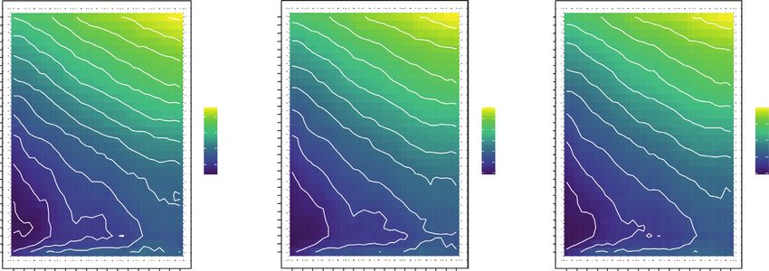
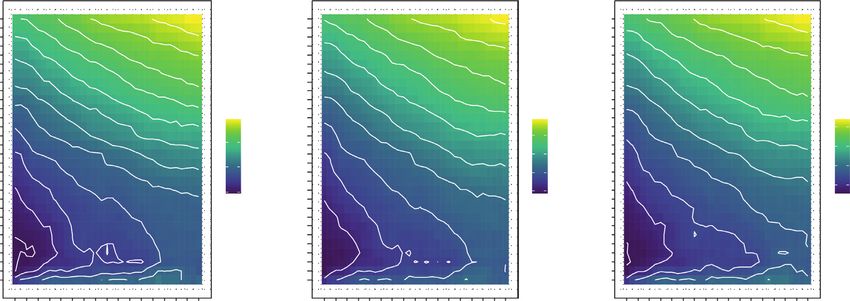
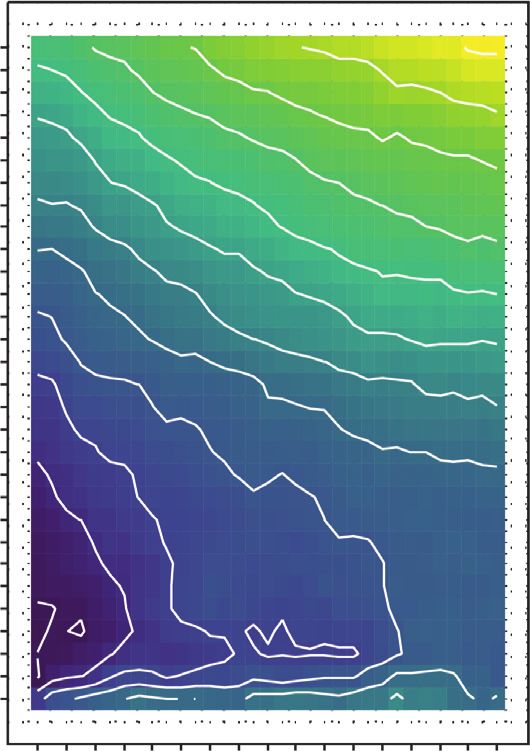
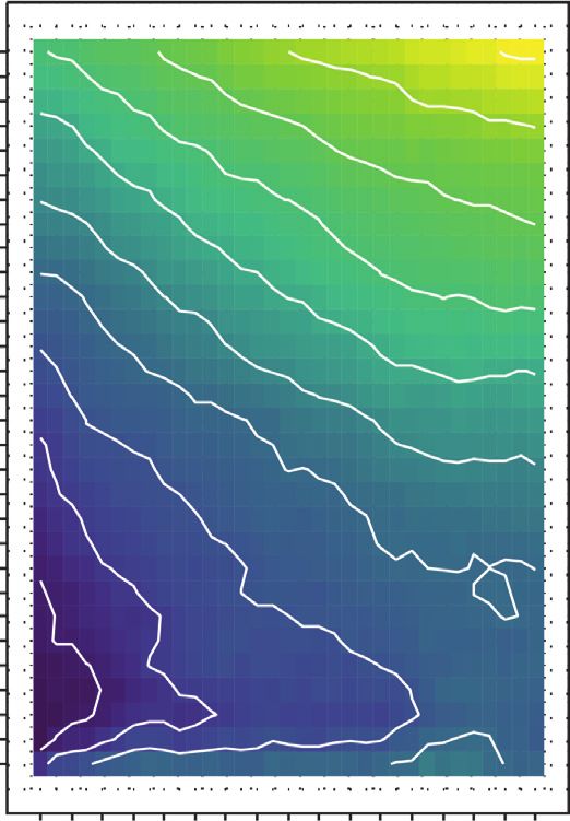
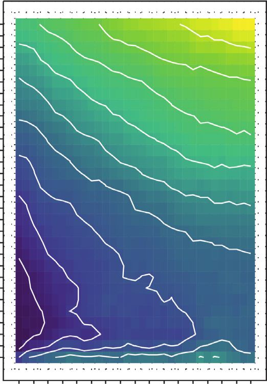
Journal of Advanced Transportation 9

 category
 0 5 10 15 20 25
 MAPE (%)
 Figure 7: Mean absolute percentage error (MAPE) results at 1-hour prediction (k � 5, lag duration � 20 min).

 Table 5: Prediction reliability based on mean absolute percentage error (MAPE).
MAPE Prediction reliability
0% ≤ MAPE < 10% Very accurate prediction
10% ≤ MAPE < 20% Accurate prediction
20% ≤ MAPE < 50% Reasonable prediction
50% > MAPE Not accurate prediction

 Table 6: Impact analysis result of road work based on actual data.
 Average travel speed at Standard deviation of Whether the
 Predicted travel Speed
Time normal conditions travel speed at normal z-score construction affects
 speed (km/h) degradation (%)
 (km/h) conditions (km/h) the speed
t+1 10:30 19.36 21.29 1.51 1.28 No —
t+2 10:35 19.48 21.65 1.50 1.45 No —
t+3 10:40 19.52 21.65 1.45 1.47 No —
t+4 10:45 19.48 21.77 0.92 2.49 No —
t+5 10:50 19.44 21.97 1.35 1.87 Yes −11
t+6 10:55 19.28 21.58 1.12 2.06 No —
t+7 11:00 18.84 21.84 1.21 2.47 Yes −11
t+8 11:05 18.64 22.35 1.60 2.32 Yes −14
t+9 11:10 18.60 22.39 1.60 2.36 Yes −17
t + 10 11:15 18.56 22.45 1.43 2.71 Yes −17
t + 11 11:20 18.72 21.94 0.89 3.60 Yes −15
t + 12 11:25 19.04 22.10 0.79 3.87 Yes −14

4. Conclusion However, this study had limitations that need im-
 provement through future studies. First, the established
It is crucial to prepare an appropriate traffic management model for predicting travel speeds in a work zone filtered the
strategy for the expected congestion level by predicting the data using the day of the week and link clusters classified
travel speed after road work to prevent congestion caused by according to road characteristics. Still, it is necessary to use
road works. This study developed a model that predicts the work type as a filter. For example, road works that block or
travel speed of the work zone using the CKNN algorithm. occupy roads largely affect traffic conditions. However, work
Furthermore, a method to grasp how much the traffic speed conducted on drains or sidewalks will only slightly influence
decreases due to road work was compared with the normal traffic conditions. Therefore, better results can be achieved if
speed pattern. the travel speed of the work zone can be predicted by
 Most proposed methodologies for short-term speed pre- considering the work type.
diction presented by several existing studies were methods for Second, a prediction model was developed using eight-
predicting speed in normal road conditions. Since roads in the month data for major arterial roads installed with traffic
work zone were entirely or partially blocked, a speed pattern information collection devices. Although the amount of data
differed from normal road conditions. Applying the proposed was not small, it was still insufficient for securing details
methodology through a case study can accurately predict the similar to the input data.
speed from the start of road construction up to an hour later. Third and last, this study used only the CKNN algorithm
Furthermore, it was likewise feasible to provide useful infor- for speed prediction. However, evaluating the appropriateness
mation for preemptive traffic congestion management by of the methodology proposed in this study compared to results
detecting the timing of link speed degradation caused by ca- predicted by other clustering methods such as support vector
pacity reduction due to road work. machines, random forests, and neural networks is required.

10 Journal of Advanced Transportation

Data Availability temporal feature extraction,” Journal of Advanced Trans-
 portation, vol. 2020, Article ID 3247847, 16 pages, 2020.
The data used to support the findings of this study are not [12] E. I. Vlahogianni, M. G. Karlaftis, and J. C. Golias, “Short-
publicly made available according to the data security policy term traffic forecasting: where we are and where we’re going,”
of Daegu Metropolitan City. Transportation Research Part C: Emerging Technologies,
 vol. 43, pp. 3–19, 2014.
 [13] L. Li, S. He, J. Zhang, and B. Ran, “Short-term highway traffic
Conflicts of Interest flow prediction based on a hybrid strategy considering
The authors declare that there are no conflicts of interest temporal-spatial information,” Journal of Advanced Trans-
regarding the publication of this paper. portation, vol. 50, no. 8, pp. 2029–2040, 2016.
 [14] B. Sun, W. Cheng, P. Goswami, and G. Bai, “Short-term traffic
 forecasting using self-adjusting k-nearest neighbours,” IET
Acknowledgments Intelligent Transport Systems, vol. 12, no. 1, pp. 41–48, 2017.
 [15] H.-C. Park, D.-K. Kim, and S.-Y. Kho, “Bayesian network for
This work was supported by the 2021 Research Fund of the freeway traffic state prediction,” Transportation Research
University of Seoul. Record: Journal of the Transportation Research Board,
 vol. 2672, no. 45, pp. 124–135, 2018.
References [16] Y. Cong, J. Wang, and X. Li, “Traffic flow forecasting by a least
 squares support vector machine with a fruit fly optimization
 [1] N. G. Polson and V. O. Sokolov, “Deep learning for short- algorithm,” Procedia Engineering, vol. 137, pp. 59–68, 2016.
 term traffic flow prediction,” Transportation Research Part C: [17] P. Wu, Z. Huang, Y. Pian, L. Xu, J. Li, and K. Chen, “A
 Emerging Technologies, vol. 79, pp. 1–17, 2017. combined deep learning method with attention-based LSTM
 [2] E. J. Kim, H. C. Park, S. Y. Kho, and D. K. Kim, “A hybrid model for short-term traffic speed forecasting,” Journal of
 approach based on variational mode decomposition for an- Advanced Transportation, vol. 2020, Article ID 8863724,
 alyzing and predicting urban travel speed,” Journal of Ad-
 15 pages, 2020.
 vanced Transportation, vol. 2019, Article ID 3958127,
 [18] F. G. Habtemichael and M. Cetin, “Short-term traffic flow rate
 12 pages, 2019.
 forecasting based on identifying similar traffic patterns,”
 [3] H. C. Park, S. Kang, S. Y. Kho, and D. K. Kim, “Investigation
 Transportation Research Part C: Emerging Technologies,
 of effects of inherent variation and spatiotemporal depen-
 dency on urban travel-speed prediction,” Journal of Trans- vol. 66, pp. 61–78, 2016.
 portation Engineering, Part A: Systems, vol. 146, no. 5, 2020. [19] H. F. Yang, T. S. Dillon, and Y. P. P. Chen, “Optimized
 [4] Y. Hou, P. Edara, and C. Sun, “Traffic flow forecasting for structure of the traffic flow forecasting model with a deep
 urban work zones,” IEEE Transactions on Intelligent Trans- learning approach,” IEEE Transactions on Neural Networks
 portation Systems, vol. 16, no. 4, pp. 1761–1770, 2014. and Learning Systems, vol. 28, no. 10, pp. 2371–2381, 2016.
 [5] Z. Zheng and D. Su, “Short-term traffic volume forecasting: a [20] Y. J. Lee and O. Min, “Long short-term memory recurrent
 K-Nearest neighbor approach enhanced by constrained lin- neural network for urban traffic prediction: a case study of
 early sewing principle component algorithm,” Transportation Seoul,” in Proceedings of the 2018 21st International Confer-
 Research Part C: Emerging Technologies, vol. 43, pp. 143–157, ence on Intelligent Transportation Systems (ITSC), pp. 1279–
 2014. 1284, Maui, HA, USA, November, 2018.
 [6] J. Guo, W. Huang, and B. M. Williams, “Adaptive Kalman [21] Z. Zhao, W. Chen, X. Wu, P. C. Y. Chen, and J. Liu, “LSTM
 filter approach for stochastic short-term traffic flow rate network: a deep learning approach for short-term traffic
 prediction and uncertainty quantification,” Transportation forecast,” IET Intelligent Transport Systems, vol. 11, no. 2,
 Research Part C: Emerging Technologies, vol. 43, pp. 50–64, pp. 68–75, 2017.
 2014. [22] W. Huang, G. Song, H. Hong, and K. Xie, “Deep architecture
 [7] S. Lee and D. B. Fambro, “Application of subset autoregressive for traffic flow prediction: deep belief networks with multitask
 integrated moving average model for short-term freeway learning,” IEEE Transactions on Intelligent Transportation
 traffic volume forecasting,” Transportation Research Record: Systems, vol. 15, no. 5, pp. 2191–2201, 2014.
 Journal of the Transportation Research Board, vol. 1678, no. 1, [23] Y. Jia, J. Wu, and Y. Du, “Traffic speed prediction using deep
 pp. 179–188, 1999. learning method,” in Proceedings of the 2016 IEEE 19th In-
 [8] D. Billings and J. S. Yang, “Application of the ARIMA models
 ternational Conference on Intelligent Transportation Systems
 to urban roadway travel time prediction-a case study,” In 2006
 (ITSC), pp. 1217–1222, Rio de Janeiro, Brazil, December, 2016.
 IEEE International Conference on Systems, Man and Cyber-
 [24] Y. Lv, Y. Duan, and W. Kang, “Traffic flow prediction with big
 netics, vol. 3, pp. 2529–2534, 2006.
 data: a deep learning approach,” IEEE Transactions on In-
 [9] A. M. Khoei, A. Bhaskar, and E. Chung, “Travel time pre-
 diction on signalised urban arterials by applying SARIMA telligent Transportation Systems, vol. 16, no. 2, pp. 865–873,
 modelling on Bluetooth data,” in Proceedings of the 36th 2014.
 Australasian Transport Research Forum (ATRF), Brisbane, [25] C. Song, H. Lee, C. Kang, and W. Lee, “Traffic speed pre-
 Australia, 2013. diction under weekday using convolutional neural networks
[10] M. Castro-Neto, Y.-S. Jeong, M.-K. Jeong, and L. D. Han, concepts,” in Proceedings of the 2017 IEEE Intelligent Vehicles
 “Online-SVR for short-term traffic flow prediction under Symposium (IV), pp. 1293–1298, Los Angeles, CA, USA, June,
 typical and atypical traffic conditions,” Expert Systems with 2017.
 Applications, vol. 36, no. 3, pp. 6164–6173, 2009. [26] C. Zhang, J. J. Q. Yu, and Y. Liu, “Spatial-temporal graph
[11] L. Kang, G. Hu, H. Huang, W. Lu, and L. Liu, “Urban traffic attention networks: a deep learning approach for traffic
 travel time short-term prediction model based on spatio- forecasting,” IEEE Access, vol. 7, pp. 166246–166256, 2019.

Journal of Advanced Transportation 11

[27] X. Luo, D. Li, Y. Yang, and S. Zhang, “Spatiotemporal traffic [42] C. Yuan and H. Yang, “Research on K-value selection method
 flow prediction with KNN and LSTM,” Journal of Advanced of K-means clustering algorithm,” D-J Series, vol. 2, no. 2,
 Transportation, vol. 2019, Article ID 4145353, 10 pages, 2019. pp. 226–235, 2019.
[28] X. Yin, G. Wu, J. Wei, Y. Shen, H. Qi, and B. Yin, “Deep [43] Transportation Research Board, Highway Capacity Manual
 learning on traffic prediction: methods, analysis and future 2010, TRB National Research Council, Washington, DC, USA,
 directions,” IEEE Transactions on Intelligent Transportation 2010.
 Systems, vol. 4, 2021. [44] A. H. Mashhadi, M. Farhadmanesh, A. Rashidi, and
[29] M. Lippi, M. Bertini, and P. Frasconi, “Short-term traffic flow N. Marković, “Review of Methods for Estimating Construc-
 forecasting: an experimental comparison of time-series tion Work Zone Capacity,” Transportation Research Record,
 analysis and supervised learning,” IEEE Transactions on In- vol. 2675, 2021.
 telligent Transportation Systems, vol. 14, no. 2, pp. 871–882, [45] A. Dhamaniya and S. Chandra, “Influence of operating speed
 2013. on capacity of urban arterial midblock sections,” International
[30] Y. Zhang, Y. Zhang, and A. Haghani, “A hybrid short-term Journal of Civil Engineering, vol. 15, no. 7, pp. 1053–1062,
 traffic flow forecasting method based on spectral analysis and 2017.
 statistical volatility model,” Transportation Research Part C: [46] T. M. Kodinariya and P. R. Makwana, “Review on deter-
 Emerging Technologies, vol. 43, pp. 65–78, 2014. mining number of cluster in K-means clustering,” Interna-
[31] Y. Wu, H. Tan, L. Qin, B. Ran, and Z. Jiang, “A hybrid deep tional Journal, vol. 1, no. 6, pp. 90–95, 2013.
 learning based traffic flow prediction method and its un- [47] C. D. Lewis, Industrial and Business Forecasting Methods: A
 Practical Guide to Exponential Smoothing and Curve Fitting,
 derstanding,” Transportation Research Part C: Emerging
 Butterworth Scientific, London, UK, 1982.
 Technologies, vol. 90, pp. 166–180, 2018.
[32] T. Liu, J. Ma, W. Guan, Y. Song, and H. Niu, “Bus arrival time
 prediction based on the K-Nearest neighbor method,” in
 Proceedings of the 2012 Fifth International Joint Conference on
 Computational Sciences and Optimization, pp. 480–483,
 Heilongjiang, China, June, 2012.
[33] M. Akbari, P. J. v. Overloop, and A. Afshar, “Clustered K
 nearest neighbor algorithm for daily inflow forecasting,”
 Water Resources Management, vol. 25, no. 5, pp. 1341–1357,
 2011.
[34] M. Kamyab, S. Remias, E. Najmi, S. Rabinia, and
 J. M. Waddell, “Machine learning approach to forecast work
 zone mobility using probe vehicle data,” Transportation Re-
 search Record: Journal of the Transportation Research Board,
 vol. 2674, no. 9, pp. 157–167, 2020.
[35] H. Wang, L. Liu, S. Dong, Z. Qian, and H. Wei, “A novel work
 zone short-term vehicle-type specific traffic speed prediction
 model through the hybrid EMD-ARIMA framework,”
 Transportation Business: Transport Dynamics, vol. 4, no. 3,
 pp. 159–186, 2016.
[36] D. R. Taylor, S. Muthiah, B. T. Kulakowski, K. M. Mahoney,
 and R. J. Porter, “Artificial neural network speed profile model
 for construction work zones on high-speed highways,”
 Journal of Transportation Engineering, vol. 133, no. 3,
 pp. 198–204, 2007.
[37] X. Jiang and H. Adeli, “Dynamic wavelet neural network
 model for traffic flow forecasting,” Journal of Transportation
 Engineering, vol. 131, no. 10, pp. 771–779, 2005.
[38] H. T. Zwahlen and A. Russ, “Evaluation of the accuracy of a
 real-time travel time prediction system in a freeway con-
 struction work zone,” Transportation Research Record,
 vol. 1803, no. 1, pp. 87–93, 2002.
[39] Q. Meng and J. Weng, “Cellular automata model for work
 zone traffic,” Transportation Research Record: Journal of the
 Transportation Research Board, vol. 2188, no. 1, pp. 131–139,
 2010.
[40] P. Cai, Y. Wang, G. Lu, P. Chen, C. Ding, and J. Sun, “A
 spatiotemporal correlative K-Nearest neighbor model for
 short-term traffic multistep forecasting,” Transportation Re-
 search Part C: Emerging Technologies, vol. 62, pp. 21–34, 2016.
[41] H. Xiaoyu, W. Yisheng, and H. Siyu, “Short-term traffic flow
 forecasting based on two-tier K-Nearest neighbor algorithm,”
 Procedia - Social and Behavioral Sciences, vol. 96, pp. 2529–
 2536, 2013.