Argos: Practical Many-Antenna Base Stations
←
→
Page content transcription
If your browser does not render page correctly, please read the page content below
Argos: Practical Many-Antenna Base Stations
                               Clayton Shepard1 , Hang Yu1 , Narendra Anand1 , Li Erran Li2 ,
                                   Thomas Marzetta2 , Richard Yang3 , and Lin Zhong1
              1                                                          2                                  3
             Rice University, Houston, TX                               Bell Labs, Murray Hill, NJ              Yale University, New Haven, CT
      {cws, hang.yu, nanand, lzhong}@rice.edu                    {erranlli, tlm}@research.bell-labs.com               yry@cs.yale.edu

ABSTRACT                                                                            resource block (i.e., time slot, spectrum channel, or code
Multi-user multiple-input multiple-output theory predicts                           sequence). Information theory shows that this limit can be
manyfold capacity gains by leveraging many antennas on                              overcome through multi-user multiple-input multiple-output
wireless base stations to serve multiple clients simultane-                         (MU-MIMO) [9]; one promising form of MU-MIMO is called
ously through multi-user beamforming (MUBF). However,                               multi-user beamforming (MUBF). With MUBF, a base sta-
realizing a base station with a large number antennas is non-                       tion employs multiple antennas to send independent data
trivial, and has yet to be achieved in the real-world.                              streams to multiple terminals in the same resource block,
   We present the design, realization, and evaluation of Ar-                        effectively improving spatial reuse. As theory shows, the
gos, the first reported base station architecture that is ca-                        more antennas a base station has, the more terminals it
pable of serving many terminals simultaneously through                              can serve simultaneously, resulting in higher spectral capac-
MUBF with a large number of antennas (M  10). De-                                  ity. Not surprisingly, the theory community is envisioning
signed for extreme flexibility and scalability, Argos exploits                       MUBF base stations with hundreds of antennas.
hierarchical and modular design principles, properly parti-                            However, building a MUBF base station with many an-
tions baseband processing, and holistically considers real-                         tennas is non-trivial. Scaling up baseband processing, clock
time requirements of MUBF. Argos employs a novel, com-                              distribution, transmission synchronization, and channel es-
pletely distributed, beamforming technique, as well as an                           timation raises serious system challenges. As a result, only
internal calibration procedure to enable implicit beamform-                         testbeds with a few antennas have been reported in the liter-
ing with channel estimation cost independent of the number                          ature, e.g., [5, 14]. Emerging wireless standards are similarly
of base station antennas. We report an Argos prototype with                         restricted to a small number of antennas and terminals. The
64 antennas and capable of serving 15 clients simultaneously.                       key question to the proposal of MUBF base stations with
We experimentally demonstrate that by scaling from 1 to 64                          many antennas remains: is it practical at all?
antennas the prototype can achieve up to 6.7 fold capacity                             In this work, we answer this question affirmatively with
gains while using a mere 1/64th of the transmission power.                          Argos 1 , a flexible base station architecture that is scalable
                                                                                    up to thousands of antennas and able to serve tens of termi-
                                                                                    nals simultaneously through MUBF. Using commercial off-
Categories and Subject Descriptors                                                  the-self radio modules, i.e., the WARP platform [4], we have
C.2.1 [Computer-Communication Networks]: Network                                    realized an Argos prototype with 64 antennas that is capable
Architecture and Design—Wireless Communication                                      of serving 15 terminals through zero-forcing and conjugate
                                                                                    MUBF. Extensive experimental characterization using this
                                                                                    prototype shows that the spectral capacity increases from
Keywords                                                                            12.7 bps/Hz when using a single-antenna to 85 bps/Hz for
Large-scale Antenna Systems (LSAS), Many-Antenna, Mas-                              Argos employing zero-forcing MUBF, and to 38 bps/Hz for
sive MIMO, Multi-User MIMO, Beamforming, Conjugate,                                 Argos employing the less computationally intensive conju-
MRT, Zero-forcing                                                                   gate MUBF, while using a mere 1/64th of the single-antenna
                                                                                    transmission power. We show that the spectral capacity
1. INTRODUCTION                                                                     grows nearly linearly with the number of base station anten-
                                                                                    nas and the number of simultaneously served terminals, as
   Due to the popularization of smartphones, tablets and
                                                                                    suggested by theory. The scale of our prototype and experi-
data-hungry applications, mobile data traffic is growing ex-
                                                                                    mentation are only limited by the number of WARP boards
ponentially, with the expectation that it will increase 18-
                                                                                    that are available to us. To the best of our knowledge, Ar-
fold within 5 years [7]. In response, wireless operators are
                                                                                    gos is the first publicly reported many-antenna MUBF base
scrambling to acquire more spectrum resources and deploy
                                                                                    station design and realization (M  10). Our work demon-
more base stations to increase spatial reuse. However, there
                                                                                    strates the feasibility of the MUBF theory community’s pro-
is a fundamental spectrum efficiency limit to existing cel-
                                                                                    posal, and presents key design principles for a scalable, flex-
lular network architectures: they are single-user systems.
                                                                                    ible, and cost-effective realization.
That is, a base station serves only one terminal in a given
                                                                                       Argos achieves its scalability and flexibility with four novel
Permission to make digital or hard copies of all or part of this work for           design principles. (i) First, Argos adopts a hierarchical
personal or classroom use is granted without fee provided that copies are           and modular design. This allows it to scale up easily by
not made or distributed for profit or commercial advantage and that copies           incrementally adding modules, e.g., WARP boards in the
bear this notice and the full citation on the first page. To copy otherwise, to
republish, to post on servers or to redistribute to lists, requires prior specific   1
permission and/or a fee.                                                             Argos is a giant with 100 eyes in Greek mythology. The
MobiCom’12, August 22–26, 2012, Istanbul, Turkey.                                   great vision of Argos is analogous to the improved capacity
Copyright 2012 ACM 978-1-4503-1159-5/12/08 ...$15.00.                               of our many-antenna base station.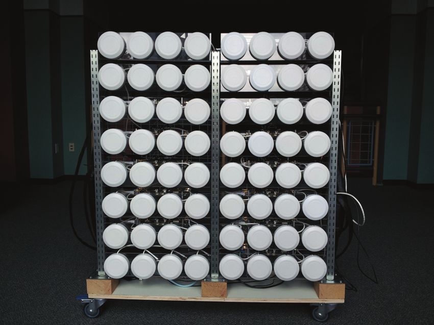
y

      Destructive

                                                                                          ĂƚĂϮ
      interference

                 =
                                     Constructive interference

                                 =
                                                       x

Figure 1: Aerial view of two antennas, represented               Figure 2: Multi-user beamforming employs base-
by two dark dots, emitting identical sine waves at               band precoding and multiple antennas to send inde-
the same frequency. The two waves perfectly rein-                pendent data streams to multiple terminals at the
force each other along the x axis (constructive inter-           same time.
ference) but completely cancel each other out along
the y axis (destructive interference). Between the                     niques to address key challenges toward realizing base
two axes the interference gradually varies, produc-                    stations with a large number of antennas, including
ing conical radiation know as a beam pattern.                          clock distribution, transmission synchronization, local-
                                                                       ized weight computation, and channel calibration.
reported prototype. As Argos scales up it can select the
                                                                   In the rest of this paper, we provide the background in
optimal beamforming algorithm by thoroughly analyzing
                                                                 Section 2. We present the design and implementation of
the performance factors and data dependencies of various
                                                                 Argos in Sections 3 and 4, respectively. In Section 5 we
MUBF techniques. (ii) Second, Argos intelligently parti-
                                                                 evaluate the real-world performance of Argos. In Sections 6
tions computation tasks among the different modules in the
                                                                 and 7 we discuss related and future work, respectively, and
hierarchy. In the downlink, data to multiple terminals is
                                                                 then conclude in Section 8.
broadcast to all antennas. Each antenna locally applies its
beamforming weights and transmits the combined signal to
all terminals simultaneously. In the uplink, I and Q sam-        2.    BACKGROUND
ples from each antenna are combined in upstream modules            We first provide some background on multi-user beam-
along the hierarchy. (iii) For very large scale operation,       forming (MUBF) and highlight the key benefits and chal-
Argos leverages a modified version of conjugate beamform-         lenges of using a large number of antennas on base stations.
ing that allows localized weight computation at each an-
tenna. Specifically, traditional conjugate beamforming re-        2.1    Beamforming Basics
quires centralized transmission power normalization, while          Beamforming utilizes multiple antennas transmitting at
Argos conducts the normalization locally at each antenna.        the same frequency to realize directional transmission. Due
This modification allows Argos to scale almost indefinitely        to constructive and destructive interference of signals from
with regard to baseband complexity. (iv) Finally, Argos          multiple transmission antennas, the signal strength received
employs a novel internal calibration procedure that allows       at different directions varies spatially, leading to a beam pat-
implicit beamforming across a large number of base station       tern, as shown in Figure 1. This beam pattern can be al-
antennas without explicit channel state information (CSI)        tered by changing the beamforming weights applied to each
estimation, enabling the real-time CSI estimation overhead       antenna, effectively altering the amplitude and phase of the
to become independent of the number of base station anten-       signal sent from that antenna. Closed-loop beamforming em-
nas. Notably, implicit beamforming requires time division        ploys CSI to calculate the beamforming weights that maxi-
duplex (TDD) operation, which is a substantial modification       mize the signal strength at intended receivers and minimize
to the frequency division duplex (FDD) systems primarily         the interference at unintended ones.
used in cellular networks currently.
   In summary, we make the following contributions to ad-        2.2    Single and Multi-user Beamforming
vance the state of the art of MUBF with many antennas:             There are two major categories of closed-loop beamform-
                                                                 ing: Single-user beamforming (SUBF) and Multi-user beam-
   • We design and realize Argos, a first-of-its-kind base        forming (MUBF). SUBF maximizes the signal strength at
     station architecture that can scale up to thousands of      a single intended receiver by using beamforming weights
     antennas serving tens of terminals with either conju-       that are the complex conjugate of the CSI, which is also
     gate or zero-forcing MUBF. We report an Argos pro-          known as maximum ratio transmission [15]. MUBF concur-
     totype with 64 antennas simultaneously serving 15 ter-      rently transmits multiple data streams, each to a different
     minals;                                                     intended receiver as shown in Figure 2. Not surprisingly,
   • Using the Argos prototype, we experimentally demon-         information theoretical studies have shown that MUBF can
     strate the real-world feasibility of base stations em-      improve spectral capacity manyfold due to its spatial multi-
     ploying many-antenna MUBF and their capability to           plexing gain.
     significantly improve capacity;                                There are many baseband techniques to realize MUBF.
                                                                 We focus on linear precoding since other methods are com-
   • The design of Argos contributes multiple novel tech-        putationally infeasible for practical systems. Let s denote
a K × 1 vector representing the data-bearing symbols to K 2.4 Challenges to Many-Antenna MUBF
users. Linear precoding creates a transmission vector s for Realizing the key benefits outlined above is, however, non-
M antennas, by multiplying the original data vector s by a trivial. Any implementation of MUBF with many antennas
M × K matrix W: s = W · s. Where W consists of the faces fundamental timing constraints imposed by the coher-
beamforming weights. ence time of the physical wireless channel. MUBF must
In this work, we study two important forms of linear- collect CSI for each terminal then use it to calculate the
precoding for MUBF: conjugate and zero-forcing. Let H beamforming weights within a small fraction of the coher-
denote the M × K channel matrix between the M base sta- ence time. Additionally, the computational complexity of
tion antennas and K concurrent terminals. Let c denote a MUBF weight calculation grows with the number of anten-
constant chosen to satisfy a transmission power constraint. nas, M , and the number of simultaneously served terminals,
Conjugate: W = Wconj = c · H∗ , where H∗ is the K. The Argos design has to address both challenges.
complex conjugate of H. In other words, conjugate beam-
forming simply takes the complex conjugate of each channel 2.4.1 CSI Estimation
coefficient in H as the beamforming weight, normalized by c. Acquisition of CSI fundamentally limits the capacity of
Indeed, it can be viewed as simultaneous single-user beam- MUBF with many antennas. MUBF with M antennas to
forming to K terminals by aggregating the signals intended serve K terminals requires CSI between every base station
for these terminals. Conjugate MUBF is sub-optimal and antenna and terminal, or M ·K channels. Importantly, all
may not perform well with a small M due to inter-terminal M ·K physical channels must be assessed within a period
interference. This method has only been recently proposed much shorter than the channel coherence time in order to be
for MUBF with a large number of antennas in [17].
−1 useful. The coherence time of a wireless channel depends on
Zero-forcing: W = c · Wzf = H∗ HT H∗ . Zero- how quickly the terminal and environment move. In cellular
forcing beamforming employs the CSI to precode the data- systems this is typically on the order of a few milliseconds,
bearing symbols so that they sum to zero, or a ‘null’, at but can drop below 500 μs [1] with vehicular mobility at or
unintended receivers. The effectiveness of zero-forcing has near the terminal. This results in a fundamental tradeoff
been experimentally demonstrated recently [5] with a small between the time spent collecting CSI, which dictates how
number of antennas (four) and terminals (four). Zero- many users can be served simultaneously, and the time al-
forcing MUBF can keep inter-terminal interference to zero located to sending beamformed data to those users. This
if K ≤ M . However, due to the required matrix inversion tradeoff is explored theoretically in [16].
the computational overhead quickly becomes infeasible for Traditionally, CSI is estimated explicitly. That is, each
real-time applications, as will be discussed in Section 2.4.2. base station antenna broadcasts a pilot to the terminal,
where the latter then uses this pilot to estimate its chan-
nel to each of the base station antennas. In order for this
2.3 Benefits of Many-Antenna MUBF channel estimation to be useful, it has to be fed back to
It is well known in information theory that MUBF with the base station in order to perform downlink beamforming.
many antennas provide the following key benefits: The reverse of this procedure is then used to find uplink CSI,
First, MUBF can greatly improve spectral capacity though feedback is unnecessary for maximum ratio combin-
through spatial reuse. Roughly speaking, the spectral ca- ing at the base station. This method thus requires O(M +K)
pacity gain from MUBF is min(M, K) [9]. A large M allows time to send pilots (one pilot from each base station antenna
the base station to serve more terminals concurrently and and terminal) and O(M ·K) estimates that need to be sent
therefore achieve higher spectral capacity. back over-the-air (M estimates from K terminals). This
Second, a very large M allows a more power-efficient and overhead is unavoidable in frequency division duplex (FDD)
cost-effective base station. The directional gain from using systems, since the physical channel is not reciprocal at dif-
a large M can be used to compensate for reduced trans- ferent frequencies.
mission power; that is, a base station can achieve the same In time division duplex (TDD) systems the physical chan-
capacity with a much lower total transmission power. Under nel is reciprocal, and thus, theoretically, CSI could be esti-
all conceivable propagation conditions doubling the number mated implicitly. That is, uplink pilots could be used to
of base station antennas permits the total radiated power perform downlink beamforming, reducing channel estima-
to be reduced by a factor-of-two with no degradation of tion overhead to O(K) and eliminating the required feed-
performance. Only when the number of antennas grows so back. This is often called implicit beamforming. However,
large that it begins to envelope the terminals or intervening in practice, the uplink and downlink channels consist of not
scatterers will this effect cease. Moreover, multi-user beam- only the physical channel, but also the channels introduced
forming distributes the total transmission power across M by the active RF components in the transmit and receive
antennas, leading to a much lower transmission power per hardware, as will be further discussed in Section 3.3.
antenna. The base station can therefore leverage cheaper
power amplifiers and simpler RF filters. This eliminates the 2.4.2 Real-time Beamforming Weight Calculation
need for active cooling, further reducing power consumption The computational complexity of MUBF weight calcula-
and total cost. tion also grows with the number of base station antennas,
Finally, since power gains are reciprocal, the preceding M , and the number of terminals, K. For conjugate MUBF,
benefit also applies to terminals. Specifically, it allows the beam weight computation is trivial. In hardware, tak-
battery-constrained terminals to use much lower transmis- ing the complex conjugate of a signal only needs a bit-flip
sion power to achieve higher capacity. and an adder. Therefore, the delay introduced by weight
In Section 5, we will experimentally demonstrate these calculation is negligible. However, zero-forcing requires the
benefits using the Argos design. computation of a matrix inverse, a calculation with the com-plexity of O(M ·K 2 ). Moreover, the inverse algorithm has estimates to be fed back to the base station. This is clearly
internal data-dependencies that limit its ability to be par- an unacceptable overhead for large-scale systems, and sug-
allelized. While the incurred latency is acceptable at small gests that Argos must employ TDD reciprocity and implicit
scales, the polynomial time nature of the inverse makes it beamforming to reduce this overhead to K pilots and elim-
very challenging for MUBF systems with a large number inate the feedback. In order to enable this, however, we
of antennas. For example, we estimate that a single 15 by must first overcome the asymmetries introduced by the RF
15 matrix inverse would require approximately 150 μs us- hardware. To accomplish this we devise a novel internal
ing a specialized high performance FPGA implementation calibration scheme, which we present in Section 3.3.
reported in [8]. 150 μs is already 30% of the 500 μs coher-
ence time specified by the LTE channel model. Moreover,
in a wideband system such as LTE, this inversion has to be
3.1.2 Beamforming Methods
performed for every 14 subcarriers [17]. Thus, while these Unfortunately, existing beamforming methods are dis-
computations may be pipelined, the true overall inversion tinctly unscalable, as they all have centralized data require-
time incurred will be far greater than 150 μs. ments and typically have polynomial time complexity, as
Additionally, existing beamforming techniques incur a discussed in Section 2.4.2.
high data transmission overhead because the channel esti- In light of this, we propose a novel beamforming method
mates and beam weights have to be exchanged between a that allows weights to be computed completely locally, at
central controller and each of the antennas. Even using each base station radio, as described in Section 3.4. Lever-
state-of-the art hardware, e.g., InfiniBand, such exchange aging this method allows additional radios to be added with-
incurs a sizable latency cost. The fastest InfiniBand bus has out requiring additional bandwidth, enabling Argos to easily
1 μs overhead per hop and 40 Gbps transfer rate [3]; it will scale up to an unprecedented number of base station anten-
incur approximately 5 μs delay per subcarrier group in a 15 nas, e.g., 1000s.
by 15 system. For a 20 MHz bandwidth this amounts to over However, while this beamforming method performs well
a 700 μs delay. Zero-forcing cannot avoid this data exchange with a very large number, e.g., 100s, of base station an-
because the inverse calculation requires the full CSI matrix, tennas serving 10s of terminals simultaneously, it is well
H. More subtly, even the simplest beamforming algorithm, known to be sub-optimal for smaller scale systems, e.g.,
conjugate, requires full knowledge of H in order to appropri- M = 30, K = 10. We demonstrate this empirically in our
ately scale the power of the steering weights. In Section 3.4, results, Section 5, where we find that zero-forcing results in
we present a novel localized conjugate beamforming method up to a 4 fold capacity increase over our method. However,
that eliminates the overhead due to data transfer between this does not account for the data transport and computa-
the central controller and antennas. tional overhead of zero-forcing, which becomes prohibitive
with a large number of users or high mobility, as described
in Section 2.4.2. Thus we conclude that in order to scale op-
3. DESIGN timally Argos must support traditional, centralized beam-
The key question we ask in this section is: how do we forming techniques for smaller scale deployments.
design a MUBF base station that can flexibly optimize its
architecture over a wide range of M and K? Before pro-
ceeding to answer it, we want to highlight its practical in- 3.1.3 Linear Precoding
terest: realistic wireless networks often have large variations Linear precoding requires each antenna to transmit a data
in many of their properties, including the financial budget stream that is the linear combination of K data streams
for the base stations, the terminal population within the with K beamforming weights. One design option is to ap-
coverage, and the data traffic volume from terminals. Tra- ply these weights centrally. Since each antenna transmits
ditional base stations can only scale their transmission power a distinct data stream, this would require the central con-
or, equivalently, their cell size, to cope with such variations. troller to deliver M I and Q sample streams to each of the
In contrast, Argos base stations can also scale the number individual radios. This approach, obviously, does not scale
of antennas to accommodate various deployment needs. well, since it requires the central controller to have an output
We argue that in order to meet these demands our many- bandwidth proportional to M . As M increases to hundreds
antenna base station must: (i) be economically affordable or even thousands, this becomes exorbitantly expensive and
with cost proportional with M , (ii) scale as both M and K eventually intractable. Thus we conclude that in any effi-
become very large, and (iii) select the optimal beamforming cient scalable design, the beamforming weights should be
technique given deployment requirements. We next present applied at the radio. This design choice conveniently allows
how our design of Argos accomplishes these attributes. all of the radios to share a common databus for downlink
transmission. In contrast, for uplink transmission, the radio
3.1 Scalability leverages the same linear precoding to apply K beamform-
The first question is: can MUBF scale up with M , the ing weights to the incoming I and Q samples. Since each
number of base station antennas? MUBF entails three dis- radio has unique weights, this again results in M unique
tinct phases: channel estimation, weight calculation, and data streams (that are K wide)! Fortunately, linear pre-
linear precoding. We explore the feasibility and design im- coding requires these streams to simply be added together;
plications of these as M scales up. conveniently, this can be done anytime two streams merge in
the architecture, thus, again, enabling a constant bandwidth
3.1.1 Channel Estimation databus. Indeed, we see that with careful design decisions
Explicit channel estimation does not scale well with M or linear precoding can scale up with constant data rate re-
K. As discussed in Section 2.4.1, explicit channel estima- quirements. Notably, there is still a need for some form of
tion typically requires M + K pilots to be sent, and M · K central controller to demodulate the data once it has beenĞŶƚƌĂů ĂƚĂĂĐŬŚĂƵů Downlink Channel: hˆi→ j
ŽŶƚƌŽůůĞƌ
ti hi → j rj
ƌŐŽƐ
,Ƶď
ƌŐŽƐ
,Ƶď
͙ ƌŐŽƐ
,Ƶď
ZĂĚŝŽŝ ZĂĚŝŽũ
ĂƐĞďĂŶĚ ĂƐĞďĂŶĚ
DŽĚƵůĞ DŽĚƵůĞ ͙ DŽĚƵůĞ
DŽĚƵůĞ ri h j →i tj
DŽĚƵůĞ
͙
͙
hˆj→i
ZĂĚŝŽ ZĂĚŝŽ ZĂĚŝŽ
DŽĚƵůĞ Uplink Channel:
Figure 3: Argos architecture: fat tree structure with Figure 4: Real channels are not reciprocal due to the
daisy-chained leaf nodes. differences in transmit and receive hardware. Note
that channel reciprocity indicates that within the
completely recombined; however this operation is latency channel coherence time the physical channel is re-
insensitive, and computationally trivial. ciprocal: hi→j = hj→i .
Thus we find that, yes, MUBF can scale up with M , but
meet latency requirements, Argos hub can simply be added
only with careful design choices and new methods for weight
to parallelize connections and reduce latency.
calculation and channel estimation.
3.3 Channel Calibration
3.2 Architecture and Topology We devise a novel, completely internal, calibration proce-
The design choices to enable scalability presented above dure to enable implicit beamforming on many-antenna base
result in two distinct components: (i) a central controller, stations through TDD channel reciprocity in order to collect
which handles modulation and demodulation, and (ii) the CSI data in constant time with respect to M .
M radio front-ends that locally calculate beam weights and For an M antenna base station to multi-user beamform
apply linear precoding. The immediate question we need to to K terminals, the base station must acquire the downlink
answer is: how do we interconnect the controller and the channel state information, ĥm→k , for all m = 1, 2, ..., M and
radios? On one hand, we can connect all the radios directly k = 1, 2, ..., K. The key challenge is to estimate the effective
to the controller. This requires the controller to have at downlink CSI ĥm→k from the uplink CSI, ĥk→m , acquired
least M ports. Since M can be dynamic and very large, this from the uplink pilot signals. However, as shown by Fig-
would be a unscalable and inefficient design choice. On the ure 4, the uplink and downlink channels are not reciprocal
other hand, we can daisy-chain all the radios serially. While due to the random phase and amplitude differences in the
scalability seems to be maximized, reliability and delay of RF hardware. This is caused by a combination of dynamic
the system are severely compromised. effects from internal clocking structures, such as dividers,
Our solution is to add hierarchies to the base station to multipliers, and PLLs, as well as static effects from manu-
improve flexibility, and simultaneously achieve a balance be- facturing deviations. Indeed, we verify that simply resetting
tween scalability, reliability, and delay. But, what type of hi- a given radio i, or even tuning to a different frequency, ran-
erarchical structure should we adopt? First we note that de- domizes the phase effects of ti and ri .
ploying M separate radios and antennas would be unwieldy, The uplink and downlink channels between any two trans-
and cost ineffective to manufacture; thus we create our first ceivers is a product of (i) the frequency response of the
level hierarchy: a module that contains one or more radio transmit hardware, (ii) the physical wireless channel, and
front-ends. Next, in order to achieve flexible, cost-effective, (iii) the frequency response of the receive hardware:
scaling we allow these modules to be connected serially; en-
abling additional modules to be added atomically with low ĥi→j = ti · hi→j · rj (1)
overhead. Finally, in order to increase reliability and reduce In order to estimate the reciprocal channel, ĥj→i , we define
end-to-end latency, we introduce the Argos hub, which al- a calibration coefficient, bi→j , between radios i and j as:
lows multiple modules to be connected in parallel. Figure 3
depicts the Argos architecture. ĥi→j ti · hi→j · rj ti · rj 1
The Argos base station enables unprecedented scalability bi→j = = = = (2)
ĥj→i ri · hj→i · tj ri · tj bj→i
and deployability, while fulfilling performance and cost con-
straints. This architecture enables the Argos base station to Notably, if both channels are measured within the coherence
scale in three directions: by adding more Argos hubs, by in- time then hj→i = hi→j due to physical channel reciprocity.
creasing the length of the module chains, and by increasing Clearly, if we know the calibration coefficient between two
the number of antennas on a module. The hierarchal archi- radios and one channel estimate, we can find the reciprocal
tecture facilitates deployments of base stations with many channel:
antennas to be flexibly distributed geographically by using ĥi→j
a single link to an Argos hub, as well as deployments of base ĥi→j = bi→j · ĥj→i or ĥj→i = (3)
bi→j
stations with a small number of antennas where the hub can
be omitted completely, and modules are simply chained to- Now let’s apply this to our scenario where we would like to
gether in series. Additionally, if chains become too long to estimate the downlink CSI from base station antenna m toterminal k (ĥm→k ) from the uplink CSI (ĥk→m ). To do this by sending pilots to and from every base station an-
we must know the M calibration coefficients between each tenna m and reference antenna 1.
base station antenna and the terminal, that is, all bm→k .
These would be impractical to find in a real-system, as esti- 2. Send K orthogonal pilots from each terminal and de-
mating bm→k requires pilots to be sent between every base termine ĥk→m .
station antenna and terminal pair, as well as feedback from
each terminal. Moreover, unless the terminal and base sta-
3. Derive all ĥm→k from 6.
tion share clocks, which is impossible in a wireless system,
their hardware transmit and receive channels drift relatively
over time, thus requiring this calibration to happen fre- 4. Use ĥm→k to calculate the beam weights, then send
quently. This approach would be counter-productive, since the beamformed data.
estimating bm→k requires downlink pilots, which could be
used to directly estimate ĥm→k . Using this process we can efficiently collect full channel state
information at the base station by sending only K termi-
3.3.1 Internal Calibration nal pilots, without any feedback from the terminals. This
We find that it is possible to internally calibrate the enables us to scale M up without any additional channel
base station relative to one of it’s antennas, e.g., antenna estimation overhead, which is a critical feature in order to
1. That is, we find all calibration coefficients bm→1 (for realize a MUBF system with many antennas.
m = 2, 3, ... M ) using Equation 2. Note that these coef- Note that the measurements of downlink and uplink have
ficients are in fact stable over long periods of time, as we to be done within the channel coherence time in order for
show in Section 5.4, since all base station antennas share hm→1 = h1→m . Since base station antennas do not move,
clocks. We also find that if we know the calibration coeffi- the channel coherence time is much larger than typical base
cient between any two radios and a reference radio, then we station to terminal coherence times. However, as we show in
can derive the direct calibration coefficient between them: Section 4.5, this calibration can easily be done well within
even highly mobile timing constraints; our prototype com-
ti ·rj
bi→j ri ·tj ty · r j pletes a single antenna pair calibration within 300 μs.
= ti ·ry = = by→j (4)
bi→y r y · tj
ri ·ty 3.4 Decentralized Beamforming
Thus if we know the calibration coefficient between our refer- In order to achieve scalable real-time beamforming weight
ence antenna and terminal k, b1→k , we can find the downlink calculation, Argos employs a novel method that allows
CSI: weights to be calculated locally at each antenna, and there-
b1→k fore avoid the unscalable data-transport overhead required
ĥk→m · = ĥk→m · bm→k = ĥm→k (5) by existing beamforming techniques. As discussed in Sec-
b1→m
tion 2.4.2, to perform traditional conjugate beamforming,
This suggests that full CSI can be found by simply send- the weights must be globally normalized so that no base
ing one pilot from each of the terminals, then just one pilot station radio exceeds its maximum power output. For ex-
from the base station’s reference antenna! Unfortunately, ample, assuming a maximum radio transmit amplitude of
however, to find b1→k we must feedback the reference an- 1, and in order to ensure at least one radio transmits at
tenna’s downlink channel estimate, ĥ1→k , from each of the maximum power:
k terminals. This significantly reduces the channel capacity,
−1
and quickly becomes infeasible for even a moderate K.
K
c= max ĥm→k (m = 1, 2, ...M ) (7)
3.3.2 Key Idea: Relative Calibration k=1
Our key idea in solving the calibration problem is that
where c is the scaling factor used in the beamforming weight
an absolutely accurate estimation of downlink CSI, ĥm→k ,
calculation (W = c · H∗ ). Global power scaling is charac-
is unnecessary. For all multi-user beamforming techniques
terized by using a single constant to scale all of the weights.
using linear precoding, it is sufficient for beamforming an-
This global scaling is necessary to maintain the ratio be-
tennas to have a relatively accurate estimation. That is, as
tween each base station antenna’s weight for a given ter-
long as each base station antenna’s CSI estimation deviates
minal, which ensures per-terminal transmission energy opti-
from the real CSI by the same multiplicative factor, multi-
mality, as proven in [15]. However, each base station antenna
user beamforming will still result in the same beam pattern.
must know either c (or H) to properly scale its own beam-
To visualize this, refer back to Figure 1; if both antennas
forming weights. This requires full CSI to be transferred
were to experience the same phase offset, the resulting spa-
from each module to the central controller, nullifying the
tial beam pattern would remain the same. Thus, we can
benefit from the aforementioned decentralization. To tackle
assume b1→k = 1:
this, we propose a local power scaling approach that closely
b1→k ĥk→m approximates global normalization.
ĥm→k = ĥk→m · ⇒ ĥm→k = = ĥk→m ·bm→1 Argos leverages a key observation that for the different ter-
b1→m b1→m
(6) minals in multi-user beamforming, the channels correspond-
This means that we estimate relative downlink CSI, ĥm→k , ing to different terminals are uncorrelated and experience
by using only uplink pilots, without any feedback! To reca- independent fading. Therefore, statistically speaking, when
pitulate, the entire CSI collection process involves 4 steps: the number of terminals is large, the actual transmission
power at each antenna is very similar. Our solution simply
1. Find all internal calibration coefficients, b1→m , offline normalizes the total transmission power locally at each baseĞŶƚƌĂů tZWDŽĚƵůĞ
boards with 64 antennas that are compactly placed on a cus-
ŽŶƚƌŽůůĞƌ tZWDŽĚƵůĞ
;,ŽƐƚWǁͬDd>Ϳ tom rack-mount platform. We note that the number of ter-
tZWDŽĚƵůĞ
ƚŚĞƌŶĞƚ
minals supported by each module is fundamentally limited
&W' ZĂĚŝŽ
;ŽŶƚƌŽůůĞĚďLJyW^Ϳ ŽĂƌĚƐ by its hardware capabilities. In the WARP boards we are us-
ƌŐŽƐ,Ƶď WŽǁĞƌW ZĂĚŝŽϭ ing, this bottleneck is the number of multipliers (328 on the
;ĐŽĚĞdĂƌŐĞƚͿ
ĂƚĂ^ǁŝƚĐŚ Virtex 2 Pro xc2vp70) [26]. We are able to use 240 of these
;
ƚŚĞƌŶĞƚͿ &W'&ĂďƌŝĐ ZĂĚŝŽϮ
ƌŐŽƐ
/ŶƚĞƌĐŽŶŶĞĐƚ multipliers to provide linear precoding for 15 terminals on
^LJŶĐWƵůƐĞ WĞƌŝƉŚĞƌĂůƐĂŶĚ ,ĂƌĚǁĂƌĞDŽĚĞů
;tZWďŽĂƌĚͿ KƚŚĞƌ/ͬK ;^ŝŵƵ>ŝŶŬͿ
ZĂĚŝŽϯ
the 4 antennas, which requires 60 complex multipliers. The
ůŽĐŬ
remaining multipliers are used by other functions, and 4 are
ŝƐƚƌŝďƵƚŝŽŶ ůŽĐŬŽĂƌĚ ZĂĚŝŽϰ unusable due to routing constraints. However, the recently
;ϵϱϮϯͿ ϭϲ
released Virtex 7 supports up to 3600 multipliers clocked
at a rate of 741 MHz; with multiplexing this would enable
Figure 5: The implementation of Argos using
16,672 complex multiplies per 40 MHz sample (neglecting
WARP boards, a laptop, an ethernet switch, and
routing overhead and other functions that require multipli-
an AD9523 based clock distribution board.
ers), which would, obviously, alleviate this bottleneck [25].
station antenna using only the CSI it measures: To the best of our knowledge, our Argos prototype is the
K −1 first publicly reported many-antenna MUBF system with
real-world feasibility. We next elaborate on our implemen-
cm = ĥm→k (m = 1, 2, ...M ) (8)
k=1
tation.
The conjugate beamforming weights are then scaled via: 4.1 Hardware and Software Platform
W = H∗ · diag(C) (9) WARP is a scalable and programmable wireless platform
for prototyping advanced wireless systems. Each WARP
Where C is the scaling vector given by Clocal = [c1 , c2 , ...cM ], board allows up to four radio daughter cards to be connected
from Equation 8; notably the globally scaled conjugate can and therefore can contribute up to four active antennas si-
also be found in this form, using Cglobal = [c, c, c, c...], from multaneously to Argos. Each radio board includes a Maxim
Equation 7. 2829 transceiver chip [18], which operates at the 2.4 or 5
We have experimentally verified the effectiveness of such GHz ISM bands with a 20 MHz bandwidth. WARP conve-
local power scaling and observed that its performance is al- niently provides a MATLAB-based framework, WARPLab,
most indistinguishable from the optimal global power scaling which allows MATLAB to control the WARP boards and
method (see Section 5), using equal transmit power for both process the transmit and receive data samples. As shown
methods. Moreover, in real deployments, since local power in Figure 5, WARPLab consists of four layers: (i) The un-
scaling ensures that each radio can utilize its full hardware derlying Simulink model that implements the custom hard-
power capacity, it can always achieve equal or greater SNR ware for controlling the FPGA board and radio boards; (ii)
than global power scaling (since it can send with greater The Xilinx Platform Studio (XPS) project that integrates
total transmit power), as proven in [22, p. 24]. Notably, if and connects all of the hardware components, including the
terminals are not approximately equidistant from the base Simulink model, the I/O cores for the serial port, Ethernet
station, then per-terminal power scaling is required to en- port, clocking, etc.; (iii) The C code that runs on the Pow-
sure fairness (preventing terminals closer to the base station erPC microprocessor, controls the hardware through mem-
from being allocated all of the transmission power), but this ory mapped I/O, and acts as an interface to the Ether-
can be done at a much coarser time scale (i.e., seconds), thus net port; (iv) The MATLAB interface that configures the
not creating additional overhead or affecting performance. boards, generates the transmit samples, and processes the
receive samples.
4. IMPLEMENTATION We have extensively customized the WARPLab frame-
In this section we provide a detailed report of our imple- work to enable hardware MUBF, transmission synchroniza-
mentation of Argos, which leverages WARP [4], commer- tion, clock synchronization, and indirect calibration among
cially available clock distribution boards, a commodity PC, base station antennas. These functionalities are essential to
and an ethernet switch. Figure 5 shows an abstract represen- for Argos to enable MUBF with many antennas.
tation of our implementation. As the first proof-of-concept
prototype, our system includes a central controller, an Ar- 4.2 Hardware MUBF
gos hub and 16 modules, each with 4 radios. The central A straightforward, and much easier approach to realize
controller consists of a single host PC, which uses MATLAB MUBF in WARPLab is to implement it in software within
to send data, weights, and control commands to the radio the MATLAB interface; this, in fact, was our first implemen-
modules. The Argos hub is comprised of a 24-port ether- tation. In this approach the beamformed baseband signal
net switch, a clock distribution board, and a WARP board, can be directly delivered to the WARP boards without the
which uses its GPIO pins to provide transmission synchro- need of linear-precoding in hardware. However, this method
nization splitting/replication. Due to the limited availability introduces major latency between the CSI collection and
of WARP boards, this board also serves as a radio module, data transmission, which increases linearly with the number
however these roles are functionally separate, and in future of base station antennas, and severely degrades performance.
generations of the Argos prototype they will be physically This is a result of the same scaling problem discussed in Sec-
separated as well. Each radio module is a single WARP tion 3.1. Therefore, we modified the WARPLab hardware
board with 4 radio daughter cards and 4 antennas. Figure 6 to enable hardware MUBF.
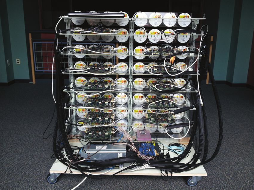
depicts the real system: the base station includes 16 WARP At each base station antenna, applying the beamform-ĞŶƚƌĂů
ŽŶƚƌŽůůĞƌ tZW
ŶƚĞŶŶĂƐ
DŽĚƵůĞƐ
ƌŐŽƐ
/ŶƚĞƌĐŽŶŶĞĐƚƐ
^LJŶĐ
ŝƐƚƌŝďƵƚŝŽŶ ůŽĐŬ
ŝƐƚƌŝďƵƚŝŽŶ
ƌŐŽƐ
ƚŚĞƌŶĞƚ
^ǁŝƚĐŚ
,Ƶď
Figure 6: The prototype of Argos with 16 modules and 64 antennas. Left: front side. Right: back side.
ing weights consists of multiplying the baseband symbol in- 4.4 Clock Synchronization
tended for each terminal, sk , by its corresponding beam- Precise inter-board clock synchronization is critical for Ar-
forming
K weight, wk , and then adding them together: sm = gos, due to its distributed modular architecture. The WARP
k=1 wk · sk where sm is the resultant beamformed signal board requires two reference clocks: a 20 MHz RF clock and
transmitted by antenna m. Multiplying the signal by a com- a 40 MHz logic/sampling clock. Both clocks can be either
plex number is equivalent to rotating the phase and scaling forwarded or driven by an external source. In addition, we
the amplitude. In hardware, this requires K registers and K discovered that the Maxim 2829 transceiver chip on the ra-
parallel complex multipliers (each complex multiplier needs dio board can use a 40 MHz clock. Therefore, we were able
4 multipliers and 2 adders) in series with 2 K input adders. to use a single external source to drive the logic clock, then
We store the beamforming weights, wk (k = 1, 2, ...K), in forward the logic clock to the reference input for the RF
memory mapped registers. This is important since it en- clock. This way, inter-board clock synchronization can be
ables the PowerPC, and in turn, the MATLAB interface to achieved in an easily manageable and scalable way.
directly control them. We leverage a commercial clock distribution evaluation
board designed for LTE, the AD9523/PCBZ, to accomplish
4.3 Transmission Synchronization this. The AD9523 provides 18 clock outputs, which we lever-
WARPLab has a default function to enable transmis- age to drive all of the radio modules. Although we haven’t
sion synchronization between multiple WARP boards. It exceeded the capacity of the AD9523, an additional clock
is achieved by using the built-in API command ”sendsync()” distribution board could be connected (as part of an addi-
in the MATLAB interface. However, due to the jitter in- tional Argos hub), which would provide 17 more outputs.
troduced by the ethernet stack, switch, and cables, such Alternatively, the existing modules can forward their clocks
synchronization can lead to a timing offset on the order to additional modules, through Argos’ multi-hop extension.
of 20 samples, depending on the ethernet switch and ca-
ble lengths, which makes accurate CSI collection and beam-
forming impossible. 4.5 Indirect Calibration
To address this challenge, we employ a WARP board to For indirect calibration, we need to estimate bm→1 =
tm ·r1
distribute the central controller’s transmission synchroniza- rm ·t1
for each antenna m with respect to the “reference
tion signal. As part of the Argos hub, this WARP node antenna,” as described in Section 3.3. Due to buffer con-
leverages directly connected, registered, GPIO to reliably straints, we implement this in a per-module iterative fash-
send the sync pulse to the radio modules. Notably, to en- ion. First, the module containing the reference antenna cali-
sure the modules receive the pulse within 1 clock cycle, the brates internally; that is, the reference antenna sends a pilot
cable lengths should all be within one wavelength, λ. With while other antennas on the module listen, then each of those
a channel bandwidth of 20 MHz, λ is 7.5 meters (40 MHz antennas sends a pilot, in turn, while the reference antenna
sampling clock), which is a very easy constraint to meet. As listens. These channel estimates are then reported to the
stated above, this WARP node serves the dual role of sync central controller so that the reference antenna’s buffer can
distribution and module, thus it “distributes” the sync to it- be overwritten. Next, the reference antenna sends a pilot
self with an effective cable length of 0. This means the other sequence while all the antennas on another module listen,
cables must be less than 7.5 meters, which is not a problem; then each of those antennas transmits a pilot, in turn, while
in our current setup the length is 2 meters. While each board the reference antenna listens. Again, the channel estimates
may have a slightly different clock phase, this phase offset is are reported to the central controller. The process is then
constant (due to the clock synchronization), and explicitly repeated for each module. The calibration procedure is very
compensated for by the beamforming algorithm. latency sensitive, as the physical channel should not change
We have modified the Simulink model, the XPS project, between transmission and reception of pilots for any antenna
and the C code to enable GPIO-based transmission synchro- pair. To address this, we implement the calibration locally
nization. Specifically, we inserted appropriate gateways and on the PowerPC in C code and leverage Argos’ transmission
registers into the Simulink model, re-mapped the GPIO pins synchronization to coordinate the send and receive phases.
to the appropriate signals in the XPS project, and disabled The resulting calibration happens within 300 μs for each an-
the traditional ethernet sync in the C code. tenna pair, which is well within the channel coherence time.90
80
70 Zero−forcing
Total Capacity (bps/hz)
Conjugate
60
Local Conj.
50 SUBF
Single Ant.
40
30
20
10
0
>ŽĐĂƚŝŽŶƐŽĨƚĞƌŵŝŶĂůƐ >ŽĐĂƚŝŽŶƐŽĨƌŐŽƐďĂƐĞƐƚĂƚŝŽŶƐ 20 30 40 50 60
Base Station Antennas
Figure 7: Environments and the locations of the Figure 8: Cell capacity as the number of base sta-
base station and terminals for for the reported ex- tion antennas (M ) increases from 16 to 64, by 4,
periments. Note that the base station leverages di- serving 15 terminals. In order to compensate for
rectional antennas in order to serve one sector. Ter- the beamforming gain, total transmission power is
minals have vertical separation as well, spanning up 1/M , implying average power per-antenna for multi-
to three floors. antenna schemes is 1/M 2 .
Another challenge we encountered while performing our typically collecting over 3000 measurements at each location,
indirect calibration approach is the significant amplitude to reliably average out performance.
variation for the channels between the reference antenna 1 To obtain the cell capacity, we aggregate the Shannon
and other antennas. This is due to the grid-like configura- capacity for each terminal, or CCell = K k=1 log(1+SIN Rk )
tion of our antenna array where different pairs of antennas where SIN Rk is the measured SINR at terminal k. We let
can have very different antenna spacings. According to our the base station transmit dummy QPSK-modulated frames
measurement, the SNR difference can be as high as 40 dB, to the terminals, which is sufficient to validate the real-world
leading to a dilemma for us to properly choose the transmis- feasibility of Argos since MUBF is a physical layer technique
sion power for the reference signal. To address this, we iso- that is orthogonal to the MAC layer and above.
late the reference antenna from the others, and place it in a To accurately measure the terminal SINR, we use the
position so that its horizontal distance to the other antennas RSSI indicator from the Maxim 2829 transceiver on the ra-
are approximately identical. Such placement of the reference dio board to report the received signal strength for each
antenna does not affect the calibration performance due to transmission, as well as the noise floor after the transmission
our calibration procedure’s isolation of the radio hardware completes. Since the radio is unable to distinguish signal
channel from the physical channel. and interference strength, we slightly stagger the transmis-
sion to the intended terminal and that to the unintended
terminals. This way we can separately measure the signal
5. EVALUATION power and interference power, and acquire the SINR accord-
Leveraging our prototype, we experimentally evaluate the ingly. To make sure the channel remains constant during the
feasibility of Argos in realistic environments. We have the transmissions we conduct our experiments in an ultra-stable
following impressive observation: compared to using a sin- environment, i.e., late at night, without moving people and
gle antenna, Argos can improve spectral capacity over 12 wireless traffic.
fold leveraging MUBF with many antennas, using equal to-
tal transmission power. With 64 antennas and 15 terminals, 5.2 Improvement of Cell Capacity
the spectral capacity can be boosted from 12.7 bps/Hz to 85 The primary purpose of our experiments is to determine
bps/Hz (6.7x) for zero-forcing MUBF, and 38 bps/Hz (3x) the capacity improvement of Argos, in order to ultimately
for conjugate MUBF, while using a mere 1/64th of the total answer the practicality of the many-antenna MUBF base
transmission power. We find that Argos easily scales from station proposal from the theory community. We report
1 to 64 base station antennas serving 1 to 15 terminals, and two sets of experiments, which evaluate the scalability with
that, in general, performance scales linearly with M and regards to the number of base station antennas, M , and the
K. Finally, we experimentally validate the performance of number of terminals, K, respectively.
our localized conjugate beamforming method, as well as our
internal calibration procedure. 5.2.1 Scaling up with M
In the first set of experiments, we vary the number of
5.1 Experimental Setup base station antennas, M , assuming a fixed number of ter-
We employ all 64 antennas at the base station to perform minals, K = 15. Figure 8 shows CCell as a function of M
MUBF to 15 concurrent terminals. We use the 2.4 GHz for a base station with a single antenna (Single Ant.), SUBF
band with a 625 kHz carrier width to avoid frequency fading (SUBF ), conjugate MUBF (Conjugate), our modified local-
effects. Since it is relatively easy to move our platform (see ized conjugate MUBF (Local Conj.), and zero-forcing MUBF
Figure 6), we tested various indoor locations (see Figure 7) (Zero-forcing). In order to compensate for the beamforming
in order to collect data from diverse environments. There gain, total transmission power is scaled by a factor of 1/M
are both LOS and NLOS channels between the base station for all five cases. This enables our experiments to separate
and terminals. We repeat our experiments multiple times, the orthogonality gain of scaling up from the well-known,90 45 15
Zero−forcing Zero−forcing Zero−forcing
80 Conjugate 40 Conjugate Conjugate
Local Conj. Local Conj. 12 Local Conj.
70 35
Total Capacity (bps/hz)
Total Capacity (bps/hz)
Total Capacity (bps/hz)
60 30
9
50 25
40 20
6
30 15
20 10 3
10 5
0 0 0
0 2 4 6 8 10 12 14 16 0 2 4 6 8 10 12 14 16 0 2 4 6 8 10 12 14 16
Number of Terminals Number of Terminals Number of Terminals
Figure 9: Cell capacity as the number of terminals K increases. Total transmission power is held constant
within each plot. Left: M = 64; Middle: M = 15; Right: M = 15 with reduced transmission power.
predictable, beamforming gain. We have the following key ditionally, the performance of conjugate flattens, and even
observations: starts to decline, as the additional interference from more
First, when M is much larger than K, both conjugate and terminals causes the average SINR to approach 0 dB.
zero-forcing MUBF increase the cell capacity as M scales up, Finally, when the transmission power is reduced, conju-
despite reducing the total transmission power proportionally gate MUBF performs relatively better than zero-forcing, as
with M . The beamforming gain from the additional anten- shown in Figure 9 Right. This is because the performance
nas compensates for the power reduction, as demonstrated of conjugate is inherently limited by interference from other
by the flat performance of SUBF, while simultaneously in- terminals, while the performance of zero-forcing is instead
creasing the natural orthogonality of the terminals. This limited by noise, since the interference is explicitly canceled.
reduces the inter-terminal interference of conjugate MUBF, It is not until the transmission power is reduced to a point
and reduces the amount of power wasted to create nulls for where interference has the same magnitude as noise that
zero-forcing MUBF. With M = 64 the improvement for con- there is a significant effect on the capacity improvement for
jugate and zero-forcing MUBF over a single antenna are 5.7x conjugate.
and 12.7x for equal power, or 3x and 6.7x for 1/64 power,
respectively. 5.3 Near-optimality of Localized Conjugate
Second, as M drops to K, i.e., M ≈ K = 15, the per-
In order to verify the viability of our localized method for
formance of zero-forcing drops steeply. This is due to the
conjugate MUBF, we implement it in Argos and compare
tightness of the degrees of freedom at the base station; zero-
it to standard conjugate MUBF with global power scaling.
forcing inevitably wastes the majority of transmission power
As shown in Figure 10, we see that our local power scaling
for interference cancelation, leading to a much reduced signal
method (Local Conj.) results in a signal power within 1.2 dB
power at the intended terminals. Later, we will show that
of global power scaling (Conjugate), but quickly approaches
when M = K this inefficiency can even result in conjugate
equivalent power as the number of terminals increases. For a
MUBF out-performing zero-forcing.
fair comparison we ensure that both methods send with the
5.2.2 Scaling up with K same transmission power, however in a practical deployment
our method will always transmit equal or more power. While
We next fix M and vary the number of terminals to see
local power scaling is less efficient for a given transmission
how capacity scales with K. In the experiments reported
power, it ensures that each base station radio is being fully
by Figures 9 Left and Middle, the total transmission power
utilized, thus more intelligently adapting to the constraints
is scaled by 1/M , similar to that in Figure 8, and is held
of real-world hardware. Furthermore, we see in Figures 8
constant regardless of K. Because the total power is split
and 9 that the performance difference between global power
among the terminals, the power per terminal is therefore
scaling (Conjugate) and local power scaling (Local Conj.) is
scaled by 1/K. In the experiment shown by Figure 9 Right,
almost indistinguishable.
we reduce the transmission power to the minimum WARP
setting in order to demonstrate how the capacity of the three
forms of MUBF are affected by power. We have the following 5.4 Stability of Indirect Calibration
observations: As described in the previous section, we implemented a
First, when M K, as shown in Figure 9 Left, capac- novel reciprocal calibration method to enable implicit beam-
ity increases approximately linearly with the number of ter- forming and efficient TDD operation. Figure 11 shows that
minals for both conjugate and zero-forcing MUBF; this is this calibration deviates from the mean angle an average of
attributable to the multiplexing gains from simultaneously less than 2.6% (maximum 6.7%), and from the mean am-
serving K terminals. plitude less than 0.7% (maximum 1.4%), over a period of
Second, conjugate beamforming initially loses capacity as 4 hours. Notably, these measurements were taken during
the number of terminals increases from 1 (SUBF) to 2 due the day with normal movement around the base station,
to the addition of interference from the other terminal, and indicating the calibration procedure is stable in real-world
thus the overwhelming drop in SINR. This loss, however, is environments. Angle deviation is calculated by difference in
quickly compensated for by the multiplexing gains. angle from average angle over π, i.e., 2.6% error is equivalent
Third, as K approaches M , the performance of zero- to 0.08 radians. This indicates that our internal calibration
forcing drops sharply as shown in Figure 9 Middle. This cor- scheme can performed very infrequently, i.e., once a day, and
roborates the second observation made in Section 5.2.1. Ad- thus has negligible performance overhead.You can also read