AUDIO-VISUAL SCENE CLASSIFICATION: ANALYSIS OF DCASE 2021 CHALLENGE SUBMISSIONS
←
→
Page content transcription
If your browser does not render page correctly, please read the page content below
Detection and Classification of Acoustic Scenes and Events 2021                                                     15–19 November 2021, Online

                                                                            AUDIO-VISUAL SCENE CLASSIFICATION:
                                                                       ANALYSIS OF DCASE 2021 CHALLENGE SUBMISSIONS

                                                                    Shanshan Wang, Toni Heittola, Annamaria Mesaros, Tuomas Virtanen

                                                                                          Computing Sciences
                                                                                      Tampere University, Finland
                                                               {shanshan.wang, toni.heittola, annamaria.mesaros, tuomas.virtanen}@tuni.fi
arXiv:2105.13675v2 [eess.AS] 20 Jul 2021

                                                                        ABSTRACT                                     more recently, ResNet [8] and EfficientNet [9] have been proposed
                                                                                                                     to further increase the performance.
                                           This paper presents the details of the Audio-Visual Scene Classi-              Motivated by the fact that we humans perceive the world
                                           fication task in the DCASE 2021 Challenge (Task 1 Subtask B).             through multiple senses (seeing and hearing), and in each individ-
                                           The task is concerned with classification using audio and video           ual domain methods have reached maturity, multimodal analysis
                                           modalities, using a dataset of synchronized recordings. This task         has become a pursued research direction for further improvement.
                                           has attracted 43 submissions from 13 different teams around the           Recent work has shown the joint learning of acoustic features and
                                           world. Among all submissions, more than half of the submitted             visual features could bring additional benefits in various tasks, al-
                                           systems have better performance than the baseline. The common             lowing novel target applications such as visualization of the sources
                                           techniques among the top systems are the usage of large pretrained        of sound in videos [10], audio-visual alignment for lip-reading [11],
                                           models such as ResNet or EfficientNet which are trained for the           or audio-visual source separation [12]. Feature learning from audio-
                                           task-specific problem. Fine-tuning, transfer learning, and data aug-      visual correspondence (AVC) [13], and more recent work that learns
                                           mentation techniques are also employed to boost the performance.          features through audio-visual spatial alignment from 360 video and
                                           More importantly, multi-modal methods using both audio and video          spatial audio [14], have shown significant improvement in perfor-
                                           are employed by all the top 5 teams. The best system among all            mance in various downstream tasks.
                                           achieved a logloss of 0.195 and accuracy of 93.8%, compared to                 Audio-visual scene classification (AVSC) is introduced in
                                           the baseline system with logloss of 0.662 and accuracy of 77.1%.          DCASE 2021 Challenge for the first time, even though research on
                                              Index Terms— Audio-visual scene classification, DCASE                  audio-visual joint analysis has been active already for many years.
                                           Challenge 2021                                                            The novelty of the DCASE task is use of a carefully curated dataset
                                                                                                                     of audio-visual scenes [15], in contrast to the use of audio-visual
                                                                                                                     material from YouTube as in the other studies. Audio-visual data
                                                                  1. INTRODUCTION                                    collected from the Youtube mostly has automatically generated la-
                                                                                                                     bel categories, which makes the data quality irregular. Besides,
                                           Acoustic scene classification (ASC) has been an important task in         most of the datasets based on material from Youtube are task spe-
                                           the DCASE Challenge throughout the years, attracting the largest          cific, e.g., action recognition [16], sport types [17], or emotion [18].
                                           number of participants in each edition. Each challenge included a         In [15], the dataset is carefully planned and recorded using the same
                                           supervised, closed set classification setup, with increasingly large      equipment, which gives it a consistent quality.
                                           training datasets [1], [2], [3], which has allowed the development of          In this paper we introduce the audio-visual scene classifica-
                                           a wide variety of methods. In recent years, the task has focused on       tion task setup of DCASE 2021 Challenge. We shortly present the
                                           robustness to different devices and low-complexity solutions [4].         dataset used in the task and the given baseline system. We then
                                                Scene classification is commonly studied in both audio and           present the challenge participation statistics and analyze the sub-
                                           video domains. For acoustic scene classification the input is typ-        mitted systems in terms of approaches. Since visual data has a large
                                           ically a short audio recording, while for visual scene classification     number of large datasets, e.g. ImageNet [6], CIFAR [19], most
                                           tasks the input can be an image or a short video clip. State-of-the-art   methods employing the visual modality are expected to use pre-
                                           solutions for ASC are based on spectral features, most commonly           trained models or transfer learning based on the pretrained models.
                                           the log-mel spectrogram, and convolutional neural network archi-          A number of resources have been listed and allowed as external data
                                           tectures, often used in large ensembles [3]. In comparison, visual        in the DCASE 2021 website.
                                           scene classification (VSC) from images has a longer history and                The paper is organized as follows: Section 2 introduces the
                                           more types of approaches, e.g. global attribute descriptors, learning     dataset, system setup and baseline system results. Section 3
                                           spatial layout patterns, discriminative region detection, and more        presents the challenge results and Section 4 gives an analysis of
                                           recently hybrid deep models [5]. The classification performance           selected submissions. Finally, Section 5 concludes this paper.
                                           for images has been significantly increased when large-scale im-
                                           age datasets like ImageNet [6] became available. Various network
                                           structures have been explored over these years, e.g. CNN [7], while          2. AUDIO-VISUAL SCENE CLASSIFICATION SETUP

                                               This work was supported in part by the European Research Council      In DCASE 2021 Challenge, an audio-visual scene classification
                                           under the European Unions H2020 Framework Programme through ERC           task is introduced for the first time. The problem is illustrated in
                                           Grant Agreement 637422 EVERYSOUND.                                        Fig.1. The input to the system is both acoustic and visual signals.
Detection and Classification of Acoustic Scenes and Events 2021 15–19 November 2021, Online
Input 2.2. Performance Evaluation
Audio
Evaluation of systems is performed using two metrics: multiclass
cross-entropy (log-loss) and accuracy. Both metrics are calcu-
lated as average of the class-wise performance (macro-average), and
ranking of submissions is performed using the log-loss. Accuracy
Video
is provided for comparison with the ASC evaluations from the chal-
lenge previous editions.
2.3. Baseline system and results
Scene Classification The baseline system is based on OpenL3 [13] and uses both audio
and video branches in the decision. The audio and video embed-
dings are extracted according to the original OpenL3 architecture,
then each branch is trained separately for scene classification based
on a single modality. The trained audio and video sub-networks
are then connected using two fully-connected feed-forward layers
Urban park
of size 128 and 10.
Metro station Audio embeddings are calculated with a window length of 1 s
and a hop length of 0.1 s, 256 mel filters, using the ”environment”
Public square content type, resulting in an audio embedding vector of length 512.
Video embeddings are extracted using the same variables as the au-
dio embedding, excluding the hop length, resulting in a video em-
Output
bedding vector of length 512. Embeddings are further preprocessed
using z-score normalization for bringing them to zero mean and unit
Figure 1: Overview of audio-visual scene classification
variance. For training the joint network, Adam optimizer [20] is
used with a learning rate set to 0.0001 and weight decay of 0.0001.
Approaches are allowed to use a single modality or both in order to Cross-entropy loss is used as the loss function. The models with
take a decision as to what scene the audio and parallel video record- best validation loss are retained. More details on the system are
ings were captured. presented in [15].
The baseline system results are presented in Table 1. In the
test stage, the system predicts an output for each 1 s segment of the
data. The results from Table 1 are different than the ones presented
2.1. Dataset in [15], because in the latter the evaluation is done for the 10 s clip.
In that case, the final decision for a clip is based on the maximum
The dataset for this task is TAU Urban Audio-Visual Scenes 2021. probability over 10 classes after summing up the probabilities that
The dataset was recorded during 2018-2019 and consists of ten the system outputs for the 1 s segments belonging to the same audio
scene classes: airport, shopping mall (indoor), metro station (un- or video clip. In DCASE challenge, the evaluation data contains
derground), pedestrian street, public square, street (traffic), travel- clips with a length of 1 s, therefore the baseline system is evaluated
ing by tram, bus and metro (underground), and urban park, from on segments of length 1 s also in development.
12 European cities: Amsterdam, Barcelona, Helsinki, Lisbon, Lon- The results in Table 1 show that the easiest to recognize was the
don, Lyon, Madrid, Milan, Prague, Paris, Stockholm, and Vienna. ”street with traffic” class, having the lowest log-loss of all classes
The audio content of the dataset is a subset of TAU Urban Acoustic at 0.296, and an accuracy of 89.6%. At the other extreme is the
Scenes 2020, in which data was recorded simultaneously with four ”airport” class, with a log-loss of 0.963 and accuracy 66.8%, and an
different devices [2]. average performance of 0.658 log-loss, with 77.0% accuracy.
The video content of the dataset was recorded using a GoPro
Hero5 Session; the corresponding time-synchronized audio data 3. CHALLENGE RESULTS
was recorded using a Soundman OKM II Klassik/studio A3 elec-
tret binaural in-ear microphone and a Zoom F8 audio recorder There are altogether 13 teams that participated to this task with one
with 48 kHz sampling rate and 24 bit resolution. The camera was to four submission entries from each team, summing up to 43 en-
mounted at chest level on the strap of the backpack, therefore the tries. Of these, systems of 8 teams outperformed the baseline sys-
captured audio and video have a consistent relationship between tem. The top system, Zhang IOA 3 [21], achieved a log loss of
moving objects and sound sources. Faces and licence plates in the 0.195 and accuracy of 93.8%. Among all submissions, 15 sys-
video were blurred during the data postprocessing stage, to meet the tems achieved an accuracy higher than 90% and a log loss under
requirements of the General Data Protection Regulation law by the 0.34. There are 11 systems which use only the audio modality,
European Union. three that use only video, and 27 multimodal systems. The best per-
The development dataset contains 34 hours of data, provided in forming audio-only system, Naranjo-Alcazar UV 3 [22], is ranked
files with a length of 10 seconds. Complete statistics of the dataset 32nd with 1.006 logloss and 66.8% accuracy. The best perform-
content can be found in [15]. The evaluation set contains 20 hours ing video-only system, Okazaki LDSLVision 1 [23], is ranked 12th
of data from 12 cities (2 cities unseen in the development set), in with 0.312 log loss and 91.6% accuracy, while the top 8 systems
files with a length of 1 second. belong to 2 teams, and are all multimodal.Detection and Classification of Acoustic Scenes and Events 2021 15–19 November 2021, Online
Baseline (audio-visual) ImageNet and Places365. Authors also propose to use embeddings
extracted from an audio-visual segment model (AVSM), to repre-
Scene class Log loss Accuracy
sent a scene as a temporal sequence of fundamental units by using
Airport 0.963 66.8% acoustic and visual features simultaneously. The AVSM sequence
Bus 0.396 85.9% is translated into embedding through a text categorization method,
Metro 0.541 80.4% and authors call this a text embedding. The combination of audio,
Metro station 0.565 80.8% video, and text embeddings significantly improves their system’s
Park 0.710 77.2% performance compared to audio-video only.
Public square 0.732 71.1% The team ranked third [23] also used audio, video and text for
Shopping mall 0.839 72.6% solving the given task. Authors use log-mel spectrogram, frame-
Street pedestrian 0.877 72.7% wise image features, and text-guided frame-wise features. For au-
Street traffic 0.296 89.6% dio, the popular pretrained CNN model trained on AudioSet is used,
Tram 0.659 73.1% with log-mel spectrogram; for video, authors select three backbones
ResNeSt, RegNet, and HRNet; finally, for the text modality, au-
Average 0.658 77.0%
thors use CLIP image encoders trained on image and text caption
pairs using contrastive learning, to obtain text-guided frame-wise
Table 1: Baseline system performance on the development dataset image features. The three domain-specific models were ensembled
using the class-wise confidences of the separate outputs, and post-
4. ANALYSIS OF SUBMISSIONS processed using the confidence replacement approach of threshold-
ing the log-loss. In this way, the system can avoid the large log-loss
A general analysis of the submitted systems shows that the most value corresponding to a very small confidence. Authors show that
popular approach is usage of both modalities, with multimodal this approach has significantly improved the log-loss results.
approaches being used by 26 of the 43 systems. Log-mel ener-
gies are the most widely used acoustic features among the submis-
4.2. Systems combinations
sions. Data augmentation techniques, including mixup, SpecAug-
ment, color jitter, and frequency masking, are applied in almost ev- Confidence intervals for the accuracy of the top systems presented
ery submitted system. The usage of large pretrained models such as in Table 2 are mostly not overlapping (small overlap between ranks
ResNet, VGG, EfficientNet trained on ImageNet or Places365 and 6 and 9). Logloss confidence intervals are ±0.02 for all systems.
fine-tuned on the challenge dataset is employed in most systems Because the systems are significantly different, we investigate some
to extract the video embeddings. The combination of information systems combinations. We first calculate the performance when
from the audio and video modalities is implemented as both early combining the outputs of the top three systems with a majority vote
and late fusion. The main characteristics and performance on the rule. The obtained accuracy is 94.9%, with a 95%CI of ±0.2. Even
evaluation set of the systems submitted by the top 5 teams are pre- though modest, this increase is statistically significant, showing that
sented in Table 2. the systems behave differently for some of the test examples.
Looking at the same systems as a best case scenario, we calcu-
4.1. Characteristics of top systems late accuracy by considering a correct item if at least one of the sys-
tems has classified it correctly. In this case, we obtain an accuracy
The top ranked system [21] adopts multimodality to solve the of 97.5% with a 95% CI of ±0.1, showing that the vast majority of
task. In the audio branch, authors employed 1D deep convolu- the test clips are correctly classified by at least one of the three con-
tional neural network and investigated three different acoustic fea- sidered systems, and that if the right rules for fusion can be found,
tures: mel filter bank, scalogram extracted by wavelets, and bark performance can be brought very close to 100%.
filter bank, calculated from the average and difference channels,
instead of left and right channels. In the video branch, authors 4.3. General trends
studied four different pretrained models: ResNet-50, EfficientNet-
b5, EfficientNetV2-small, and swin transformer. Authors use the An analysis over the individual modalities among the submissions
pretrained model trained on ImageNet, and fine-tune it first on reveals that video-based methods have advantages over audio-based
Places365, then on TAU Urban Audio-Visual Scenes 2021 dataset. ones. The best audio-only model achieves a logloss of 1.006 and ac-
RandomResizedCrop, RandomHorizontalFlip, and Mixup data aug- curacy of 66.8%, while the best video-only model has a much lower
mentation techniques are also applied. This approach takes the top logloss of 0.132 and much higher accuracy of 91.6%. This is due to
4 ranks, with the best system being based on the combination of several reasons. Firstly, image classification domain has a relatively
EfficientNet-b5 and log-mel acoustic features, a hybrid fusion com- longer history than the audio scene classification, which allowed
prised of model-level and decision-level fusion. the development of mature and large pretrained models with mil-
The team ranked on second place [24] used an audio-visual lions of parameters, for example, CNNs, ResNet, VGG, Efficient-
system and explored various pretrained models for both audio and Net and so forth. Secondly, the large-scale image datasets and the
video domain. The systems also include data augmentation through variety of the available image data, such as ImageNet, COCO and
SpecAugment, channel confusion, and pitch shifting. Specifically, so forth, help making the model more robust. Thirdly, image do-
for the audio embedding, authors investugated use of the pretrained main has attracted much attention throughout the years, including
VGGish and PANN networks, both trained on AudioSet, with trans- large numbers of participants in various challenges, such as Kaggle
fer learning applied to solve the AVSC task. Authors propose use challenges, therefore promoting the rapid development of this field.
of FCNN and ResNet to extract high-level audio features, to bet- Even though the audio-only models achieve lower performance
ter leverage the acoustic presentations in these models. For the than video-only ones, the best performance was obtained by sys-
video embeddings, authors adopt the pretrained model trained on tems which combined the two modalities. This validates our initialDetection and Classification of Acoustic Scenes and Events 2021 15–19 November 2021, Online
Rank Team Logloss Accuracy (95% CI) Fusion Methods Model Complexity
1 Zhang IOA 3 0.195 93.8% (93.6 - 93.9) early fusion 110M
5 Du USTC 4 0.221 93.2% (93.0 - 93.4) early fusion 373M
9 Okazaki LDSLVision 4 0.257 93.5% (93.3 - 93.7) audio-visual 636M
10 Yang THU 3 0.279 92.1% (91.9 - 92.3) early fusion 121M
16 Hou UGent 4 0.416 85.6% (85.3 - 85.8) late fusion 28M
24 DCASE2021 baseline 0.662 77.1% (76.8 - 77.5) early fusion 711k
Table 2: Performance and general characteristics of top 5 teams (best system of each team). All these systems use both audio and video.
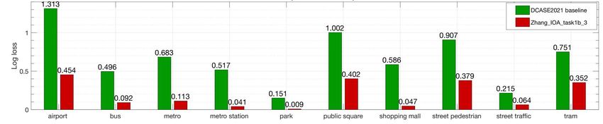
Figure 2: Class-wise performance comparison between the top 1 system and the baseline system on the evaluation set.
airport the systems have consistent behavior and good generalization prop-
bus erties. Most of the system performance shows only a very slight
metro drop in performance on the evaluation dataset, which is explained
metro station by the data from two cities unseen in training.
The confusion matrix of the top system is shown in Fig.3. In
Actual
park
public square general, the top system performs very good in all classes; the mini-
shopping mall mum class performance is 84%, and the highest is 100%. In partic-
street pedestrian ular, the system achieves the best performance in ”park”(100) and
street traffic
excellent in ”metro station”(99), ”metro”(98), ”shopping mall”(98),
tram
”street traffic”(98), ”bus”(97). We observe that ”airport” class is
airport bus metro me_st park pu_sq sh_ma st_pe st_tr tram mostly misclassified as ”shopping mall”(12); ”public square” is of-
Predicted ten misclassified as ”street pedestrian”(10) and ”street traffic”(6);
and ”tram” is mostly misclassified as ”bus” and ”metro”. This be-
Figure 3: Confusion matrix of the top-performing system [21]. havior is rather intuitive, since inside the airport there are many
shops which may resemble ”shopping mall”, and inside the ”tram”
there are mostly seats and people which may also resemble ”bus”
idea that joint modeling of audio and visual modalities can bring
or ”metro”.
significant performance gain compared to state-of-the-art uni-modal
A bar plot comparison of the class-wise performance on the
systems.
evaluation set between the baseline and the top system is shown in
An analysis of the machine learning characteristics of the sub-
Fig.2. It can be seen that the top system has significantly higher per-
mitted systems reveals that there is a direct relationship between the
formance in all classes, especially ”airport” (logloss 0.859 smaller)
performance and the model complexity, that is, in general, the top-
and ”public square” (logloss 0.6 smaller). Some similarities be-
performing systems tend to have more complex models with larger
tween the baseline system and the top system can be observed in the
numbers of trainable parameters. Indeed, Spearman’s rank correla-
bar plot, with ”park” being the easiest to classify among all classes
tion coefficient [25] between the model complexity and system rank
for both systems, and ”airport” being the most difficult one.
is 0.75, indicating that they are highly correlated. Considering both
complexity and the performance, the baseline system is a balanced
choice with a satisfactory performance. 5. CONCLUSIONS AND FUTURE WORK
The choice of evaluation metrics does not affect the ranking
drastically. We found that the top team stays the same position, Audio-visual scene classification task was introduced in the
the system Okazaki LDSLVision 4 would jump to the second in- DCASE2021 challenge for the first time, and had a high number
stead of the third spot, Hou UGent 4 would drop to the seventh participants and submissions. More than half of the submissions
instead of the fifth, and Wang BIT 1 would jump to the tenth from outperformed the baseline system. Multimodal approaches were
the thirteenth. The Spearman’s rank correlation between accuracy widely applied among the submissions, and also achieved the best
and logloss indicates a very strong correlation, at 0.93. performance compared to uni-modal methods. The choice of mod-
In general, no significant changes have been found in terms of els used by the top systems reveals that large and well-trained pre-
the system performance between the development dataset and the trained models are important for this task, while data augmentation
evaluation dataset, which shows that the dataset is well balanced and and fine-tuning techniques help making the system more robust.Detection and Classification of Acoustic Scenes and Events 2021 15–19 November 2021, Online
6. REFERENCES 2021 IEEE International Conference on Acoustics, Speech
and Signal Processing (ICASSP). IEEE, 2021. [Online].
[1] A. Mesaros, T. Heittola, and T. Virtanen, “TUT database Available: https://arxiv.org/abs/2011.00030
for acoustic scene classification and sound event detection,”
[16] K. Soomro, A. Zamir, and M. Shah, “UCF0101: A dataset
in 24th European Signal Processing Conference 2016 (EU-
of 101 human actions classes from videos in the wild,” arXiv
SIPCO 2016), Budapest, Hungary, 2016.
preprint arXiv:1212.0402, 2012.
[2] ——, “A multi-device dataset for urban acoustic scene clas-
[17] R. Gade, M. Abou-Zleikha, M. Graesboll Christensen, and
sification,” in Proc. of the Detection and Classification of
T. B. Moeslund, “Audio-visual classification of sports types,”
Acoustic Scenes and Events 2018 Workshop (DCASE2018),
in Proc. of the IEEE Int.Conf. on Computer Vision (ICCV)
November 2018, pp. 9–13.
Workshops, December 2015.
[3] ——, “Acoustic scene classification in DCASE 2019 chal- [18] S. Zhang, S. Zhang, T. Huang, W. Gao, and Q. Tian, “Learning
lenge: Closed and open set classification and data mismatch affective features with a hybrid deep model for audio–visual
setups,” in Proc. of the Detection and Classification of Acous- emotion recognition,” IEEE Trans. on Circuits and Systems
tic Scenes and Events 2019 Workshop (DCASE2019), New for Video Technology, vol. 28, no. 10, pp. 3030–3043, 2018.
York University, NY, USA, October 2019, pp. 164–168.
[19] A. Krizhevsky, G. Hinton, et al., “Learning multiple layers of
[4] T. Heittola, A. Mesaros, and T. Virtanen, “Acoustic scene features from tiny images,” 2009.
classification in dcase 2020 challenge: generalization across
devices and low complexity solutions,” arXiv preprint [20] J. Kingma, D.and Ba, “Adam: A method for stochastic op-
arXiv:2005.14623, 2020. timization,” in Proc. Int.Conf. on Learning Representations,
2014.
[5] L. Xie, F. Lee, L. Liu, K. Kotani, and Q. Chen, “Scene
recognition: A comprehensive survey,” Pattern Recognition, [21] M. Wang, C. Chen, Y. Xie, H. Chen, Y. Liu, and P. Zhang,
vol. 102, p. 107205, 2020. [Online]. Available: http://www. “Audio-visual scene classification using transfer learning and
sciencedirect.com/science/article/pii/S003132032030011X hybrid fusion strategy,” DCASE2021 Challenge, Tech. Rep.,
June 2021.
[6] J. Deng, W. Dong, R. Socher, L.-J. Li, K. Li, and L. Fei-Fei,
“ImageNet: A Large-Scale Hierarchical Image Database,” in [22] J. Naranjo-Alcazar, S. Perez-Castanos, M. Cobos, F. J. Ferri,
CVPR09, 2009. and P. Zuccarello, “Task 1B DCASE 2021: Audio-visual
scene classification with squeeze-excitation convolutional re-
[7] A. Krizhevsky, I. Sutskever, and G. E. Hinton, “Imagenet clas- current neural networks,” DCASE2021 Challenge, Tech. Rep.,
sification with deep convolutional neural networks,” Advances June 2021.
in neural information processing systems, vol. 25, pp. 1097–
1105, 2012. [23] S. Okazaki, K. Quan, and T. Yoshinaga, “Ldslvision sub-
missions to dcase’21: A multi-modal fusion approach for
[8] K. He, X. Zhang, S. Ren, and J. Sun, “Deep residual learning audio-visual scene classification enhanced by clip variants,”
for image recognition,” in Proceedings of the IEEE conference DCASE2021 Challenge, Tech. Rep., June 2021.
on computer vision and pattern recognition, 2016, pp. 770–
778. [24] Q. Wang, S. Zheng, Y. Li, Y. Wang, Y. Wu, H. Hu, C.-H. H.
Yang, S. M. Siniscalchi, Y. Wang, J. Du, and C.-H. Lee, “A
[9] M. Tan and Q. Le, “Efficientnet: Rethinking model scaling for model ensemble approach for audio-visual scene classifica-
convolutional neural networks,” in International Conference tion,” DCASE2021 Challenge, Tech. Rep., June 2021.
on Machine Learning. PMLR, 2019, pp. 6105–6114.
[25] C. Spearman, “The proof and measurement of association
[10] R. Arandjelovic and A. Zisserman, “Objects that sound,” in between two things,” The American journal of psychology,
Proceedings of the European Conference on Computer Vision vol. 15, no. 1, pp. 72–101, 1904.
(ECCV), September 2018.
[11] J. S. Chung, A. Senior, O. Vinyals, and A. Zisserman, “Lip
reading sentences in the wild,” in 2017 IEEE Conf. on Com-
puter Vision and Pattern Recognition (CVPR), 2017, pp.
3444–3453.
[12] H. Zhao, C. Gan, A. Rouditchenko, C. Vondrick, J. McDer-
mott, and A. Torralba, “The sound of pixels,” in Proc. of
the European Conf. on Computer Vision (ECCV), September
2018.
[13] R. Arandjelovic and A. Zisserman, “Look, listen and learn,”
in 2017 IEEE International Conference on Computer Vision
(ICCV), 2017, pp. 609–617.
[14] P. Morgado, Y. Li, and N. Vasconcelos, “Learning represen-
tations from audio-visual spatial alignment,” arXiv preprint
arXiv:2011.01819, 2020.
[15] S. Wang, A. Mesaros, T. Heittola, and T. Virtanen, “A curated
dataset of urban scenes for audio-visual scene analysis,” inYou can also read