CFD Modelling of Tidal Bores: Development and Validation Challenges - UQ eSpace
←
→
Page content transcription
If your browser does not render page correctly, please read the page content below
LENG, X., SIMON, B., KHEZRI, N., LUBIN, P., and CHANSON, H. (2019). "CFD Modelling of Tidal Bores:
Development and Validation Challenges." Coastal Engineering Journal, Vol. 60, No. 4, pp. 423-436 (DOI:
10.1080/21664250.2018.1498211) (ISSN 0578-5634).
CFD Modelling of Tidal Bores: Development and Validation Challenges
by
Xinqian LENG ( ), Bruno SIMON ( ) ( ) ( ), Nazanin KHEZRI (1) (4), Pierre LUBIN (2) (*),
1 1 2 3
and Hubert CHANSON (1) (2)
(1) The University of Queensland, School of Civil Engineering, Brisbane QLD 4072, Australia
(2) Université de Bordeaux, I2M, Laboratoire TREFLE, 16 avenue Pey-Berland, Pessac, France
(3) Currently: Université Aix-Marseille, France
(4) Currently: GHD, Brisbane QLD 4000, Australia
(*) Corresponding author: E-mail: p.lubin@u-bordeaux.fr
Abstract
A tidal bore is a natural estuarine phenomenon forming a positive surge in a funnel shaped river mouth during the early
flood tide under spring tide conditions and low freshwater levels. The bore propagates upstream into the lower
estuarine zone and its passage may induce some enhanced turbulent mixing, with upstream advection of suspended
material. Herein the flow field and turbulence characteristics of tidal bores were measured using both numerical (CFD)
and physical modelling. This joint modelling approach, combined with some theoretical knowledge, led to some new
understanding of turbulent velocity field, turbulent mixing process, Reynolds stress tensor, and tidal bore
hydrodynamics. The numerical CFD tool Thétis was used herein. Thétis is a CFD model using the volume of fluid
technique (VOF) to model the free-surface and Large Eddy Simulation technique (LES) for the turbulence modelling.
Physical data sets were used to map the velocity and pressure field and resolve some unusual feature of the unsteady
flow motion. A discussion will be provided to explain why a detailed validation process is crucial, involving a physical
knowledge of the flow. Comparison of the numerical model results and experimental data over broad ranges of
conditions for the same flow is mandatory. The validation process from 2D to 3D will be commented and difficulties
will be highlighted.
Keywords: Tidal bores, Computational fluid dynamics (CFD), Numerical modelling, Validation processes, Physical
experiments.
1. INTRODUCTION
A tidal bore is a positive surge occurring naturally during spring tide with large tidal range forming in a funnel-shaped
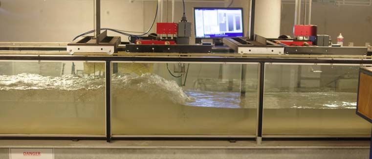
river mouth and propagating upstream (Fig. 1). Figure 1 presents photographs of tidal bores in France and China (Left)
and of tidal bores in a relatively large-size laboratory facility (19 m long, 0.7 m wide) (Left). The tidal bore induces
enhanced turbulent mixing and a large amount of sediment load during its inland propagation. Laboratory observations
and computational fluid dynamics (CFD) calculations highlighted a number of seminal features of tidal bore
investigations. Several common features were observed. First, a tidal bore is a positive surge, a compression wave, and
a hydraulic jump in translation (LIGHTHILL, 1978; LUBIN and CHANSON, 2017). It is a hydrodynamic shock, with
no net mass flux, i.e. it is not a periodic wave. A tidal bore is an unsteady, highly turbulent flow motion. The shape of
1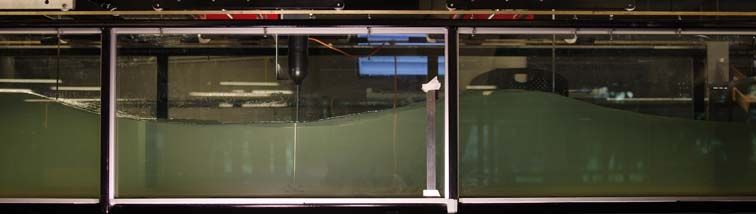
LENG, X., SIMON, B., KHEZRI, N., LUBIN, P., and CHANSON, H. (2019). "CFD Modelling of Tidal Bores:
Development and Validation Challenges." Coastal Engineering Journal, Vol. 60, No. 4, pp. 423-436 (DOI:
10.1080/21664250.2018.1498211) (ISSN 0578-5634).
the tidal bore is governed by its Froude number, defined as Fr = (V1+U)/(gA1/B1)1/2, where V1 is the initial velocity
positive downstream, U is the bore celerity positive upstream, g is the gravity acceleration, A1 is the initial cross-section
area and B1 is the initial free-surface width (CHANSON, 2012). In a rectangular channel, the bore Froude number
equals Fr = (V1+U)/(gd1)1/2 with d1 the initial flow depth. For an undular non-breaking bore, Fr < 1.2 to 1.3
(PEREGRINE, 1966; CHANSON, 2010), while Fr > 1.5 to 1.8 for a breaking bore. An undular bore with some
breaking (also called breaking bore with secondary waves) is observed for an intermediate range of Froude numbers.
For a breaking bore, the bore celerity is not truly constant, rather it constantly fluctuates about a mean value (LENG
and CHANSON, 2015a). The fluctuations in bore celerity are large in both transverse and longitudinal directions, with
ratio of standard deviation to mean value greater than unity. The bore roller toe perimeter constantly fluctuates with
time and space, so it is not a straight line (CHANSON, 2016; WANG et al., 2017).
A breaking tidal bore is a tri-phase flow, with three distinct phases flowing: liquid (water), solid (sediment) and gas
(air) (CHANSON, 2013; LENG and CHANSON, 2015b). The three-phase nature of tidal bore flow was never
accounted for, although it has been reported by numerous photographs and illustrations. In most tidal bore occurrences,
the sediment load is large and turbulent modulation in sediment-laden flows must be significant (Fig. 1B, Left).
Suspended sediment concentrations (SSCs) in excess of 20 kg/m3 were observed in the field (Garonne, Sélune, Sée,
Qiantang Rivers). For such large suspended sediment loads, and together with rheological data (FAAS 1995,
CHANSON et al. 2011; KEEVIL et al. 2015), a non-Newtonian flow behaviour could be expected, i.e. typically a non-
Newtonian thixiotropic flow. To date, the non-Newtonian behaviour of sediment-laden tidal bore flow was never
considered nor modelled, and no study was undertaken in three-phase flows with high sediment and air content despite
the high practical relevance.
(A) Undular bores - (Left) Undular bore of the Dordogne River bore at Saint Pardon (France) on 30 October 2015,
propagating from left to right; (Right) Laboratory undular bore (Fr = 1.2) propagating from left to right
2LENG, X., SIMON, B., KHEZRI, N., LUBIN, P., and CHANSON, H. (2019). "CFD Modelling of Tidal Bores:
Development and Validation Challenges." Coastal Engineering Journal, Vol. 60, No. 4, pp. 423-436 (DOI:
10.1080/21664250.2018.1498211) (ISSN 0578-5634).
(B) Breaking bores - (Left) Qiantang River bore at Meilvba (China) on 22 September 2016, propagating from top right
to bottom left; (Right) Looking downstream at incoming breaking bore (Fr = 2.2) in laboratory
Fig. 1- Photographs of tidal bores in the field (Left) and in laboratory (Right).
A tidal bore is technically a hydraulic jump in translation (CHANSON 2009). There are analogies between stationary
hydraulic jumps, positive surges, compression waves and estuarine bores (tidal bores, tsunami bores) as discussed
recently (WANG et al. ,2017; LUBIN and CHANSON, 2017). In the present contribution, we wish to focus on tidal
bore propagation in natural channel. The literature on positive surges in hydropower canals is relevant, albeit validation
of numerical modelling is restricted by the very limited number of field data sets, mostly free-surface observations (e.g.
CUNGE 1966, PONSY and CARNONNELL 1967).
Historically, numerical modelling of positive surges and tidal bores was based upon one-dimensional and two-
dimensional depth-averaged models (PREISSMANN and CUNGE 1967; MADSEN et al. 2005). Since 2009,
computational fluid dynamics (CFD) modelling of tidal bore flows was conducted at the University of Bordeaux, with
detailed validation data sets obtained at the University of Queensland in large-size flumes. The aim of this paper is to
present the latest CFD developments and validation results, as well as to discuss challenges associated with the
validation process. It will be argued that a detailed validation process is crucial, and requires a solid expert knowledge
of the physical processes.
2. CFD MODELLING DEVELOPMENTS
In the breaking bore simulation, the difficulties with free surface modelling include significant air-water interactions at
the free surface and numerical diffusion caused by large deformations of the air-water interface. LUBIN et al. (2010a,b)
presented two dimensional numerical results, solving the Navier-Stokes equations in air and water, coupled with a
subgrid scale turbulence model (Large Eddy Simulation – LES). The general trends of the flow behaviour were
observed: the bore front passage was shown to be associated with a rapid flow deceleration, coupled with a sudden
increase in water depth. The numerical data were qualitatively in agreement with field and laboratory data. These
encouraging preliminary results demonstrated the need for realistic inflow conditions, to be specified at the inlet
boundary. Numerical simulations of two-dimensional (2D) undular and breaking bores in an open channel were
performed by KHEZRI (2014) to investigate the characteristics of turbulent flow beneath the bores. Some unsteady
two-phase tidal bore motion was simulated for further understanding of the tidal bore. The simulations were performed
3LENG, X., SIMON, B., KHEZRI, N., LUBIN, P., and CHANSON, H. (2019). "CFD Modelling of Tidal Bores:
Development and Validation Challenges." Coastal Engineering Journal, Vol. 60, No. 4, pp. 423-436 (DOI:
10.1080/21664250.2018.1498211) (ISSN 0578-5634).
with flow conditions comparable to the experimental studies of KHEZRI (2014) (Table 1), and these experimental data
were used to validate the CFD modelling. The flow characteristics were chosen to be similar to the experiments: the
bore was generated through the sudden closure of a Tainter gate at the downstream end of the channel, and the bore
travelled against an initially steady flow. The complete closure of the gate resulted in a breaking bore (Fr = 1.32 to 1.4)
and the gate closure with partial opening underneath the gate produced an undular bore (Fr = 1 to 1.30). The pressure
distribution measured beneath the breaking bore was comparable to experimental estimates. The vortical structures
were mapped and visualised using the numerical data. The observation of coherent structures, and their upward motion
beneath the breaking bore in the numerical study, could explain the observed upward particle motion observations
during the breaking bore experiments. On another hand, when considering the free-surface and velocities evolutions,
discrepancies were observed. The numerical modelling was conducted with the same inflow conditions and
downstream/upstream boundary conditions as the physical experiments, in order to generate targeted breaking and
undular bores. That is, the initial flow depth, depth-averaged velocity, and the gate opening after closure (for the
undular case) were identical. With these conditions, the numerical modelling yielded slightly different tidal bore
characteristics. It was acknowledged that the numerical and experimental modelling of undular bore, did not show
exactly similar characteristics; although the numerical simulation was configured based on the experimental modelling.
The Froude number and bore celerity were found to be higher in the numerical simulation compared to the
experimental modelling (Table 1). Table 1 compares some characteristics of undular bore in the experimental and
numerical modelling. It was speculated that the differences could be explained by both experimental and numerical
errors. It was also suggested that other differences between experimental and numerical modelling could be caused by
the bore generation process. Indeed, the undular bore generation in the physical channel needed some mechanical
trigger from downstream, which could have some effects on the bore characteristics. Ultimately, the flow
characteristics were chosen with similar initial condition as experiments, the closest possibly, so the results were still
comparable, as the numerical results showed similar trends as experimental results.
Table 1 - Tidal bore flow conditions modelled by KHEZRI (2014) in a 0.5 m wide rectangular channel with rough bed
Bore type Model Bore celerity U (m.s-1) Fr
Breaking Physical 0.86 1.36
Numerical (CFD) 1.01 1.53
Undular Physical 0.63 1.17
Numerical (CFD) 0.83 1.43
CHANSON et al. (2012) discussed and proved a need for more realistic unsteady inflow conditions (JARRIN et al.,
2006) to be specified at the inlet boundary. The three-dimensional (3D) numerical simulation of a weak breaking bore
generation and propagation was presented for the first time. Some simulation time was first required for the injected
turbulent boundary condition to propagate along the rectangular open-channel. Then, the wall boundary condition was
set at the left side of the numerical domain to mimic the experimental closing gate. In the breaking bore simulation, the
difficulties with free surface modelling include significant air-water interactions at the free surface and numerical
diffusion caused by large deformations of the air-water interface.
SIMON (2014) focused on 2D and 3D numerical simulations of undular bores, to investigate the characteristics of
turbulent flow beneath the bores, considering partial and complete gate opening. The steady flow turbulence was re-
4LENG, X., SIMON, B., KHEZRI, N., LUBIN, P., and CHANSON, H. (2019). "CFD Modelling of Tidal Bores:
Development and Validation Challenges." Coastal Engineering Journal, Vol. 60, No. 4, pp. 423-436 (DOI:
10.1080/21664250.2018.1498211) (ISSN 0578-5634).
created by using a synthetic eddy method (SEM) on the domain inlet. 3D undular bores were generated for the first
time, analysing the effect of an incoming turbulent river flow. The 3D free surface evolution showed some
characteristic bore features with the appearance of cross-waves for the simulation realised with a bore Froude number
of 1.26. The global evolution of bores was similar to experimental observations (CHANSON 2010). Depending on the
bore generation method, the unsteady velocity data showed different evolution patterns. The simulations with a fully
closed gate showed successive flow reversals beneath crests and troughs. The simulations with a partially closed gate
showed velocity reversal zones close to the bed and sidewalls following the bore propagation. Close to the bed, the
intensity of flow reversal reached maximum values of up to 1.7 and 0.9 times the initial steady flow velocity for the
case with a completely and partially closed gate respectively. For the case with a gate partially closed, coherent
structures were observed in the wake of the velocity reversals beneath the bore front close to the bed. In three
dimensions, the flow generated complex structures. The coherent structures were advected downstream following the
flow motion and tended to move upwards in the water column, in agreement with qualitative experimental
observations. The comparison of 2D and 3D simulations showed that the 2D simulations were insufficient to reproduce
all the bores features, such as cross waves and coherent structures, but could give some basic results concerning the
global flow patterns. Nonetheless, the findings stressed the importance of studying the flow in three dimensions. The
comparison of simulations with and without turbulence in the initial steady flow showed that the initial turbulence had a
limited effect on the free surface evolution and the bore celerity, but could have a more significant effect on the
velocity field. SIMON (2014) observed some limitation with the numerical simulation. The case with a partially closed
gate presented some difference with earlier experimental results, as the initial steady flow conditions between
experiment and numerical simulation differed. These deviations were attributed to the mesh size selected upon the
available computing resources. In the initially steady flow, some limitations also appeared with spurious velocities
sometimes appearing next to the downstream boundary, which could sometimes disappear once the bore was generated.
Nevertheless, the numerical work presented a simultaneous characterisation of both the free surface and velocity,
validated for each case with experimental data.
3. CFD MODEL CONFIGURATION FOR TIDAL BORE SIMULATIONS
3.1 Numerical model
New CFD modelling was conducted with a focus on 3D initially steady flow and 2D breaking bore simulations, over a
relatively wide range of flow conditions. The finite volume method is used to discretise the system of equations. The
interface tracking was achieved by applying the volume of fluid technique (VOF). The VOF method is relatively simple
and can be used to describe accurately the flow interface with rupture and reconnection. The basic idea is to locate the
two media by a continuous colour function C indicating the phase rate of presence, C = 0 for the air and C = 1 for the
water. The function C depends on the fluid velocity and its evolution is described by an advection equation. No
boundary condition is used between air and water, it is classically assumed that the free-surface is located at C = 0.5.
The governing equations, i.e. the Navier-Stokes equations and continuity equation, were discretised on a staggered grid
with a finite-volume method. The implicit temporal discretisation was utilised. The non-linear convective terms were
discretised by an upwind-centred scheme, whereas a second-order centred scheme was chosen for the approximation of
the viscous terms. The velocity/pressure coupling was performed with a pressure connection method. The method
5LENG, X., SIMON, B., KHEZRI, N., LUBIN, P., and CHANSON, H. (2019). "CFD Modelling of Tidal Bores:
Development and Validation Challenges." Coastal Engineering Journal, Vol. 60, No. 4, pp. 423-436 (DOI:
10.1080/21664250.2018.1498211) (ISSN 0578-5634).
consists of two stages of velocity prediction and pressure correction in the Navier-Stokes system. The turbulence
modelling was performed using large eddy simulation technique (LES). The free surface tracking was achieved by
volume of fluid method (VOF) to enable achieving the interface reconnections in the modelling of two dimensional two
phase flows.
The code was parallelized using the MPI library. The linear system was solved using the HYPRE parallel solver and
preconditioning library. A BICGStab solver (Bi-Conjugate Gradient Stabilized solver associated with a point Jacobi
pre-conditioner) was used to solve the precondition steps and a GMRES solver (associated with a multi-grid pre-
conditioner) for the correction steps. All the equations and details concerning the numerical tool are described by
LUBIN and GLOCKNER (2015).
Two and three-dimensional numerical domains were used in this study and partitioned into 24 subdomains (one
processor per subdomain). For 2D models, the computation time was roughly 24-36 hours. For 3D models, the
computation time was 12-24 hours for 2 to 4 s of flow. The simulations have been restarted about five times to get the
presented physical times (at least 10 s).
3.2 Initial conditions
The 2D numerical domain was 12 m in the longitudinal (stream-wise) direction and 1 m in the vertical direction (Fig.
2). A no-slip condition was imposed at the lower boundary (z = 0 m) and a Neumann condition was used at the upper
boundary (z = 1 m). At the end of domain (x = 12 m), a wall boundary was imposed to act like a closed gate to
reproduce the experimental generation process. The opening under the gate hout could be set to introduce a Neumann
condition between the bed (z = 0 m) and the bottom of the gate (z = hout). For 2D models, the initial conditions were
composed of a water trapezoid, with higher depth at inlet (din) to mimic the backwater effect in the physical gradually-
varied flow. For 3D models, the depths at inlet and outlet were the same i.e. a water rectangular cuboid. The initial and
boundary parameters used in the 2D and 3D models were selected from experimental studies by LENG and
CHANSON (2016a).
The 3D model was built upon the 2D model configuration, by adding a third dimension being the transverse y
dimension. The coordinate y was positive towards the left sidewall and the 3D numerical domain was 0.7 m wide. In
this case, no-slip conditions were applied to both lateral walls and bottom of the domain. Table 2 documents detailed
configurations of the 2D and 3D numerical models. In the table, So stands for the channel slope in the longitudinal
direction. The opening under the gate after rapid closure is denoted hout. Table 3 summarises the experimental flow
conditions corresponding to the three Froude numbers modelled in laboratory (Fr = 1.2, 1.5, 2.1). The reference depth d
and celerity U was taken at the velocity sampling location, which was located 9.6 m upstream of the gate for both
physical and numerical channels.
6LENG, X., SIMON, B., KHEZRI, N., LUBIN, P., and CHANSON, H. (2019). "CFD Modelling of Tidal Bores:
Development and Validation Challenges." Coastal Engineering Journal, Vol. 60, No. 4, pp. 423-436 (DOI:
10.1080/21664250.2018.1498211) (ISSN 0578-5634).
(A) Numerical domain configurations; X is the distance from the left boundary (i.e. gate) of the numerical domain; x is
the distance from the upstream end of the physical channel
(B) Experiment in the 19 m long 0.7 m wide at the University of Queensland: Fr = 1.5, hout = 0, So = 0
Fig. 2 - Definition sketch of numerical domain configurations and comparison with the physical model of LENG and
CHANSON (2016a,2017a,b).
The 2D and 3D numerical domains are discretized into non-regular Cartesian cells. For numerical models denoted
2D_Fr1.2, in the longitudinal direction, the grid is clustered with a constant grid size ∆x=0.005 m from x = 0 m to 4 m,
then increasing exponentially for x = 4-12 m. In the vertical direction, the smallest mesh grid resolution ∆zmin = 0.005
m is set at the bottom, while exponentially increasing between z = 0-0.1 m, then the grid is clustered with a constant
grid size ∆z = 0.005 m in the free-surface region (z = 0.1-0.5 m). An exponentially-varied mesh was used above z = 0.5
m up to z = 1 m starting from a minimum ∆z = 0.005 m.
For numerical models denoted 2D_Fr1.5, in the longitudinal direction, the grid is clustered with a constant grid size
∆x=0.005 m throughout the length of the numerical domain (x = 0-12 m). In the vertical direction, the grid is clustered
with a constant grid size ∆z=0.005 m throughout the height of the numerical domain (z = 0-1 m).
For numerical models denoted 2D_Fr2.1, in the longitudinal direction, the grid is clustered with a constant grid size
∆x=0.005 m from x = 0 m to 4 m, then increasing exponentially for x = 4-12 m. In the vertical direction, the smallest
mesh grid resolution ∆zmin = 0.005 m is set at the bottom, spacing constantly between z = 0-0.5 m, then the gird
increased exponentially from z = 0.5-1 m with 50 grids.
For all 3D numerical models, in the longitudinal direction, the grid is clustered with a constant grid size ∆x=0.005 m
from x = 0 m to 4 m, then increasing exponentially for x = 4-12 m. In the vertical direction, the smallest mesh grid
7LENG, X., SIMON, B., KHEZRI, N., LUBIN, P., and CHANSON, H. (2019). "CFD Modelling of Tidal Bores:
Development and Validation Challenges." Coastal Engineering Journal, Vol. 60, No. 4, pp. 423-436 (DOI:
10.1080/21664250.2018.1498211) (ISSN 0578-5634).
resolution ∆z min = 0.0025 m is set at the bottom, constantly spacing between z = 0-0.5 m, then exponentially
increasing between z = 0.5-1 m with 50 grids. A constant spacing mesh was used in the transverse y direction
throughout from y = 0-0.7 m with ∆y = 0.0035 m.
Table 2. Initial configuration of the 2D and 3D numerical simulations of tidal bores in a 0.7 m wide smooth channel
Reference Domain (m) Mesh grid Fr Q So din (m) dout (m) hout (m) Bore type
density (m3/s)
2D_Fr1.2 12×1 1600×100 1.2 0.101 0 0.208 0.19 0.071 Undular
2D_Fr1.5 12×1 2400×200 1.5 0.101 0 0.18 0.16 0 Breaking
2D_Fr2.1 12×1 1600×140 2.1 0.101 0.0075 0.1 0.1 0 Breaking
3D_Fr1.5 12×1×0.7 1600×250×200 1.5 0.101 0 0.17 0.17 0 Breaking
3D_Fr2.1 12×1×0.7 1600×250×200 2.1 0.101 0.0075 0.093 0.093 0 Breaking
Table 3. Flow conditions of the experimental data used to validate the numerical model (LENG and CHANSON 2016a)
Reference Fr Q (m3/s) So d1 (m) U (m) Bore type Instrumentation
EA_Fr1.2 1.2 0.101 0 0.210 0.71 Undular ADMs and ADV
EA_Fr1.5 1.5 0.101 0 0.180 1.13 Breaking ADMs and ADV
EA_Fr2.1 2.1 0.101 0.0075 0.100 1.00 Breaking ADMs and ADV
4. RESULTS
4.1 CFD simulation of the initially steady flow
During the physical experiments of tidal bores, the initially steady flow was left to run for at least 60 seconds before
rapidly closing the downstream Tainter gate. A clear understanding of the flow physics and turbulent dynamics in the
initially steady flow was essential as the tidal bores were very sensitive to the turbulent character of the inflow (KOCH
and CHANSON, 2009; CHANSON et al., 2012). Past numerical CFD modelling on tidal bores included the works of
KHEZRI (2014) and SIMON (2014) provided limited to no information on the initially steady flow properties before
the bore arrival. As a result, the poor agreement in velocity fields between the 3D numerical simulation and
experimental data could not be addressed due to the lack of validation in the steady flow period. The present study
expanded on previous works by simulating the initially steady flow before generating the bore for at least 10 seconds.
The steady flow characteristics simulated by the numerical CFD models were examined and compared to experimental
results corresponding to the same flow conditions. The boundary layer properties and development were validated
against physical experiments.
Herein, the inflow turbulence was generated using the synthetic eddy method (SEM) based on the view of turbulence as
a superposition of coherent structures (JARRIN et al., 2006, 2009; CHANSON et al., 2012). The method was robust
and computationally inexpensive by generating a stochastic signal with prescribed mean velocity, Reynolds stresses,
time and length scale distributions. The prescribed input parameters were selected based upon the experimental results
of the simulated flow conditions. The turbulent eddies were injected from the upstream end of the numerical domain
and convected downstream.
Figure 3A shows the time-variations of the longitudinal velocity component Vx of the initially steady flow before the
generation of breaking bore with Fr = 1.5. The coloured curves denoted instantaneous velocity at different vertical
8LENG, X., SIMON, B., KHEZRI, N., LUBIN, P., and CHANSON, H. (2019). "CFD Modelling of Tidal Bores:
Development and Validation Challenges." Coastal Engineering Journal, Vol. 60, No. 4, pp. 423-436 (DOI:
10.1080/21664250.2018.1498211) (ISSN 0578-5634).
elevations z. The simulation was conducted for approximately 16 seconds (dimensionless time t×(g/d1)1/2 ~ 121), and
the injected turbulence arrived at the probing point X = 9.6 m at approximately 2 s (dimensionless time t×(g/d1)1/2 ~
15). The instantaneous longitudinal velocity demonstrated clearly some low frequency fluctuations, with a period of
oscillation of roughly between 3 to 4 seconds (t×(g/d1)1/2 ~ 26). The time-averaged longitudinal velocity at different
vertical elevations were presented in Figure 3B. The numerical results were compared to experimental data of the same
flow condition (EA_Fr1.5) and a 1/N power law (Fig. 3B and 3C). The experimental results were collected using an
ADV at 200 Hz then time-averaged over 30 s. The numerical results were time-averaged over 14 s, starting from the
time at which turbulence arrived at the probing point. Using a cut-off frequent fcut = 1 Hz, the low-pass filtered
experimental time series (Fig. 3C) showed close agreement with the numerical time series (Fig. 3A) both qualitatively
and quantitatively. Both experimental and numerical data highlighted larger oscillations in longitudinal velocity at
lower vertical elevation (z/d1 ~ 0.06), compared to higher vertical elevation (z/d1 ~ 0.8). The period of large oscillation
in velocity signal was similar for both numerical and experimental data.
The vertical profile of longitudinal velocity simulated by the numerical model showed a clear boundary layer, which
was partially developed. The thickness of the numerical boundary layer was approximately 0.5d1, which was
comparable to the experimental finding. Within the boundary layer, the numerical data matched closely with the
theoretical power law next the bed (z/d1 < 0.1) and near the outer edge of the boundary layer (z/d1 = 0.3 to 0.5). At the
highest vertical elevation (z/d1 = 0.862), the numerical data showed a large deviation from the experimental value, as
well as the overall trend of the rest of the numerical data. Similar error at highest vertical elevation were also observed
for steady flow with another flow condition (Fig. 4B) and in previous findings by SIMON (2014). Despite the highest
vertical elevation, the numerical data showed a close agreement with the experimental data and theoretical curve for the
rest of the vertical profile.
z/d1 = 0.034 z/d1 = 0.211 EA_Fr1.5
z/d1 = 0.064 z/d1 = 0.387 Power law N=9
z/d1 = 0.122 z/d1 = 0.858 3D_Fr1.5
1.05 1.05
1 1
0.95 0.95
0.9 0.9
Vx/Vmax
Vx/Vmax
0.85 0.85
0.8 0.8
0.75 0.75
0.7 0.7
0.65 0.65
0.6 0.6
0 20 40 60 80 100 120 140 0 0.1 0.2 0.3 0.4 0.5 0.6 0.7 0.8 0.9 1 1.1
t(g/d1)1/2 z/d1
(A, Left) Time-variations of the instantaneous longitudinal velocity (CFD numerical 3D_Fr1.5)
(B, Right) Time-averaged vertical profile of the longitudinal velocity (CFD numerical, experimental and power law
theoretical)
9LENG, X., SIMON, B., KHEZRI, N., LUBIN, P., and CHANSON, H. (2019). "CFD Modelling of Tidal Bores:
Development and Validation Challenges." Coastal Engineering Journal, Vol. 60, No. 4, pp. 423-436 (DOI:
10.1080/21664250.2018.1498211) (ISSN 0578-5634).
z/d1 = 0.062 (200 Hz) z/d1 = 0.062 (low-pass filtered fcut = 1 Hz)
1.5
z/d1 = 0.833 (200 Hz) z/d1 = 0.833 (low-pass filtered fcut = 1 Hz)
1.35
1.2
1.05
Vx/Vmax
0.9
0.75
0.6
0.45
0.3
40 48 56 64 72 80 88 96
t(g/d1)1/2
(C) Time-variations of the longitudinal velocity (experimental EA_Fr1.5): instantaneous data sampled at 200 Hz and
low-pass filtered data using a cut-off frequency fcut = 1 Hz
Fig. 3 – Time-variations and time-averaged vertical profile of the longitudinal velocity component during the initially
steady flow for breaking bore with Fr = 1.5; Comparison between numerical, experimental and theoretical results;
Numerical configuration 3D_Fr1.5; Experimental configuration EA_Fr1.5.
z/d1 = 0.062 z/d1 = 0.282 EA_Fr2.1
z/d1 = 0.097 z/d1 = 0.527 Power law N=11
z/d1 = 0.158 z/d1 = 0.712 3D_Fr2.1
1.05 1.05
1.02 1.02
0.99 0.99
0.96 0.96
0.93 0.93
Vx/Vmax
Vx/Vmax
0.9 0.9
0.87 0.87
0.84 0.84
0.81 0.81
0.78 0.78
0.75 0.75
0 20 40 60 80 100 120 0 0.1 0.2 0.3 0.4 0.5 0.6 0.7 0.8 0.9 1
t(g/d1)1/2 z/d1
(A) Left: time-variations of the instantaneous longitudinal velocity (CFD numerical 3D_Fr2.1)
(B) Right: Time-averaged vertical profile of the longitudinal velocity (CFD numerical, experimental and power law
theoretical)
Fig. 4 – Time-variations and time-averaged vertical profile of the longitudinal velocity component during the initially
steady flow for breaking bore with Fr = 2.1; Comparison between numerical, experimental and theoretical results;
Numerical configuration 3D_Fr2.1; Experimental configuration EA_Fr2.1.
10LENG, X., SIMON, B., KHEZRI, N., LUBIN, P., and CHANSON, H. (2019). "CFD Modelling of Tidal Bores:
Development and Validation Challenges." Coastal Engineering Journal, Vol. 60, No. 4, pp. 423-436 (DOI:
10.1080/21664250.2018.1498211) (ISSN 0578-5634).
4.2 CFD simulation of the unsteady bore propagation
During the physical experiments, free-surface measurements were conducted non-intrusively using a series of acoustic
displacement meters (ADMs), located at different longitudinal x locations along the channel centreline, where x is the
distance from the channel's upstream end. The ADMs were calibrated against point gauge measurements before the
experiments and sampled steady and unsteady flows at a sampling rate of 200 Hz. The physical experiments started
with steady flows, running for at least 60 s before a downstream gate was rapidly closed, generating a tidal bore which
propagated upstream. The rapidly-closing Tainter gate was located at downstream end (x = 18.1 m). Each experimental
run was terminated after the bore travelled to the upstream intake. To perform ensemble-averaged measurements, at
least 25 experimental runs were repeated for each flow condition listed in Table 3, and the results were ensemble-
averaged.
The 2D unsteady numerical model started at the gate closure, i.e. initial condition t = 0 at gate closure, when tidal bores
were generated. The simulation was stopped after the bore reached the inlet of numerical domain, and was considered
one run. Due to limitation in computational time and capacity, each flow condition was only simulated for one run by
the numerical CFD model. During the simulation, free-surface elevation was recorded at a number of longitudinal
locations in the numerical channel. These locations were equivalent to the ADMs locations in the physical channel.
Figure 5 shows a comparison between the free-surface elevations varying with time as reproduced by the numerical
model and measured by the experiments (ensemble-averaged and single run data). The flow condition shown by Figure
5 corresponded to tidal bores with the highest tested Froude number (Fr = 2.1), with the horizontal axis origin
t×(g/d1)1/2 = 0 at gate closure.
Close to the gate (Fig. 6A), the free-surface showed an abrupt rise as the breaking bore was generated and propagated.
Immediately upstream of the gate at x = 17.81 m, the free-surface was modelled reasonably well by the numerical
simulation. The timing of sudden increase in free-surface, the gradient of the increase and the maximum depth reached
after were very similar, compared between numerical models and experimental data. After the first peak in depth,
however, the numerical data started to decrease in depth and deviate from the experimental data. Further upstream at x
= 14.96 m, the free-surface variations from the simulation and experiments showed some marked differences The
numerical depth started to increase much earlier compared to the experimental data, and showed jumps when increasing
with time rather than a smooth continuous slope as seen in the experimental data. Although the peak in depth reached
by the numerical data compared well in values to the experimental data, the trend of time-variations after the peak was
very different from the experimental results. Further upstream, the numerically simulated bore reached x = 8.5 m much
earlier than the experimental observation. The time difference between the bore arrival time of the numerical and
experimental results was approximately Δt×(g/d1)1/2 = 28, corresponding to a dimensional value of Δt = 2.82 s. The
simulation of breaking bore with Fr = 1.5 showed similar lag in predicting the bore arrival time at upstream locations,
compared to the experimental data. However, the lag was much smaller than 2D_Fr2.1 (Δt ~ 0.6 s for 2D_Fr1.5).
Despite the time difference, the numerical data was similar to the experimental results at x = 8.5 m, with larger
oscillations in depth as it turned to rise rapidly, and slightly overestimated the depth after the bore passage.
For undular bores with Fr = 1.2 (Fig. 6), the numerical and experimental results showed close agreements in terms of
the free-surface evolution with time near the gate and also further upstream (x = 8.5 m). The bore celerity was well
modelled by the numerical simulation and almost no time lag was observed between the numerical and experimental
11LENG, X., SIMON, B., KHEZRI, N., LUBIN, P., and CHANSON, H. (2019). "CFD Modelling of Tidal Bores:
Development and Validation Challenges." Coastal Engineering Journal, Vol. 60, No. 4, pp. 423-436 (DOI:
10.1080/21664250.2018.1498211) (ISSN 0578-5634).
data in terms of the bore arrival time, even further upstream at x = 8.5 m. As the undular bore propagated, the free-
surface elevation increased smoothly with a train of secondary waves following the first wave front. The experimental
data showed a decrease in wave height for the secondary undulations. This was also highlighted by the numerical data.
The highest wave amplitude was associated with the bore front, namely the first wave crest immediately after the bore.
x = 17.81 m 2D_Fr2.1 x = 14.96 m EA_Fr2.1
x = 14.96 m 2D_Fr2.1 x = 17.81 m single run
x = 17.81 m EA_Fr2.1 x = 14.96 m single run
3.6
3.2
2.8
2.4
2
d/d1
1.6
1.2
0.8
0.4
0
0 10 20 30 40 50 60 70 80 90 100
t(g/d1)1/2
(A) Close to the gate
x = 8.5 m 2D_Fr2.1 x = 8.5 m EA_Fr2.1 x = 8.5 m single run
3.6
3.2
2.8
2.4
2
d/d1
1.6
1.2
0.8
0.4
0
0 25 50 75 100 125 150 175
t(g/d1)1/2
(B) Further upstream
Fig. 5 – Comparison of free-surface elevation variation with time between CFD numerical data, ensemble-averaged
experimental data and single run experimental data at different longitudinal x positions (A) close to the gate and (B)
further upstream; Time t = 0 at gate closure; Numerical configuration 2D_Fr2.1; Experimental configuration EA_Fr2.1.
12LENG, X., SIMON, B., KHEZRI, N., LUBIN, P., and CHANSON, H. (2019). "CFD Modelling of Tidal Bores:
Development and Validation Challenges." Coastal Engineering Journal, Vol. 60, No. 4, pp. 423-436 (DOI:
10.1080/21664250.2018.1498211) (ISSN 0578-5634).
x = 17.81 m 2D_Fr1.2 x = 14.96 m EA_Fr1.2
x = 14.96 m 2D_Fr1.2 x = 17.81 m single run
x = 17.81 m EA_Fr1.2 x = 14.96 m single run
1.8
1.6
1.4
1.2
1
d/d1
0.8
0.6
0.4
0.2
0
0 10 20 30 40 50 60 70 80
t(g/d1)1/2
(A) Close to the gate
x = 8.5 m 2D_Fr1.2 x = 8.5 m EA_Fr1.2 x = 8.5 m single run
1.8
1.6
1.4
1.2
1
d/d1
0.8
0.6
0.4
0.2
0
0 10 20 30 40 50 60 70 80 85
t(g/d1)1/2
(B) Further upstream
Fig. 6 – Comparison of free-surface elevation variation with time between CFD numerical data, ensemble-averaged
experimental data and single run experimental data at different longitudinal x positions (A) close to the gate and (B)
further upstream; Time t = 0 at gate closure; Numerical configuration 2D_Fr1.2; Experimental configuration EA_Fr1.2.
The numerical simulation showed an underestimation in the wave amplitude near the gate shortly after the generation (x
= 17.81 m), however tended to overestimation the amplitudes as the numerical bore travelled further upstream (x =
14.96 m & 8.5m). The numerical models were unable to reproduce the secondary waves with the same periodicity as
13LENG, X., SIMON, B., KHEZRI, N., LUBIN, P., and CHANSON, H. (2019). "CFD Modelling of Tidal Bores:
Development and Validation Challenges." Coastal Engineering Journal, Vol. 60, No. 4, pp. 423-436 (DOI:
10.1080/21664250.2018.1498211) (ISSN 0578-5634).
the experimental model (Fig. 6). The period of the secondary waves in the numerical simulation was much shorter than
the experimental waves.
Overall, the free-surface variations with time modelled by the 2D simulation agreed very well with the experimental
data close to the gate at generation, qualitatively and quantitatively. The height of the bore at generation tended to be
lower for bores simulated numerically, as shown by results for all Froude numbers (Fr = 1.2, 1.5 and 2.1). As the bore
propagated upstream, the numerical model tended to overestimate the bore celerity, resulted in early increase in depth at
the same longitudinal location when compared to the experimental observation. This time difference in bore arriving
time became more significant as the bore travelled further upstream, albeit less significant for small Froude number. In
the 2D numerical simulation, velocity components in the longitudinal and vertical directions were recorded at X = 9.6
m in the numerical channel, equivalent to x = 8.5 m in the physical channel, and at a number of vertical elevations z.
The unsteady turbulent velocity characteristics in the physical channel were measured using an acoustic Doppler
velocimeter (ADV) located at x = 8.5 m mid-channel. The ADV was equipped with a three-dimensional side-looking
head, capable of recording velocity components in the longitudinal, vertical and transverse directions. The velocity
measurements were conducted at different vertical elevations within the initially steady flow depth. Experiments
repeated 25 times for each flow condition and the results were ensemble-averaged. Velocity characteristics recorded by
the numerical and physical models were compared for the same vertical elevation and flow condition. Figure 7 presents
results for breaking bore with Fr = 2.1. Note that the velocity and depth data of the experimental results were
synchronised manually with the numerical velocity data. The time t = 0 started at the numerical gate closure.
For all vertical elevations, the longitudinal velocity showed rapid deceleration associated with the bore passage,
highlighted by both numerical and physical data (Fig. 7A). The gradient of the deceleration was well predicted by the
numerical model at all vertical elevations as compared to the experimental data. At the lowest vertical elevation (z/d1 =
0.1), a longitudinal recirculation was observed in both numerical and physical data, marked by negative values reached
at the end of the deceleration phase. The numerical recirculation occurred at a small time lag after the experimental
recirculation. Nevertheless, the magnitudes of the two recirculation velocities were comparable. After the minimum
value reached at the end of longitudinal deceleration, the velocity data measured by the physical experiments fluctuated
around zero. The frequency of such fluctuations was relatively high (f ~ 30 Hz) and the magnitudes were low
(~0.05V1). On the other hand, the numerical data showed some large periodic oscillation in longitudinal velocity
shortly after the end of the rapid deceleration. The period of the oscillation was as high as 1.6 s and the mean amplitude
of such fluctuation was approximately 0.3V1. This large periodic oscillation was considered not sensible, and possibly
due to the constraint of the two dimensionality of the numerical model.
14LENG, X., SIMON, B., KHEZRI, N., LUBIN, P., and CHANSON, H. (2019). "CFD Modelling of Tidal Bores:
Development and Validation Challenges." Coastal Engineering Journal, Vol. 60, No. 4, pp. 423-436 (DOI:
10.1080/21664250.2018.1498211) (ISSN 0578-5634).
z/d1 = 0.1 2D_Fr2.1 z/d1 = 0.1 EA_Fr2.1 dmedian 2D_Fr2.1
z/d1 = 0.4 2D_Fr2.1 z/d1 = 0.4 EA_Fr2.1 dmedian EA_Fr2.1
z/d1 = 0.8 2D_Fr2.1 z/d1 = 0.8 EA_Fr2.1
3.2 4.5
2.8 4
2.4 3.5
2 3
1.6 2.5
Vx/V1
d/d1
1.2 2
0.8 1.5
0.4 1
0 0.5
-0.4 0
0 25 50 75 100 125 150 175
t(g/d1)1/2
(A) Longitudinal velocity Vx
mascaret_fr21_vitesse_x2.txt
z/d1 = 0.1 2D_Fr2.1 z/d1 = 0.1 EA_Fr2.1 dmedian 2D_Fr2.1
mascaret_fr21_vitesse_x2
z/d1 = 0.4 2D_Fr2.1 z/d1 = 0.4 EA_Fr2.1 dmedian EA_Fr2.1
z/d1 = 0.8 2D_Fr2.1 z/d1 = 0.8 EA_Fr2.1
3.2 4.5
2.8 4
2.4 3.5
2 3
1.6 2.5
Vz/V1
d/d1
1.2 2
0.8 1.5
0.4 1
0 0.5
-0.4 0
0 25 50 75 100 125 150 175
t(g/d1)1/2
(B) Vertical velocity Vz
Fig. 7 – Comparison of velocity variation with time between CFD numerical data and ensemble-averaged experimental
data for the (A) longitudinal velocity Vx and (B) vertical velocity Vz; Time t = 0 at gate closure; Velocity data offset by
+1 every higher elevation; Numerical configuration 2D_Fr2.1; Experimental configuration EA_Fr2.1.
15LENG, X., SIMON, B., KHEZRI, N., LUBIN, P., and CHANSON, H. (2019). "CFD Modelling of Tidal Bores:
Development and Validation Challenges." Coastal Engineering Journal, Vol. 60, No. 4, pp. 423-436 (DOI:
10.1080/21664250.2018.1498211) (ISSN 0578-5634).
z/d1 = 0.1 2D_Fr1.2 z/d1 = 0.1 EA_Fr1.2 dmedian 2D_Fr1.2
z/d1 = 0.4 2D_Fr1.2 z/d1 = 0.4 EA_Fr1.2 dmedian EA_Fr1.2
z/d1 = 0.8 2D_Fr1.2 z/d1 = 0.8 EA_Fr1.2
3.2 2.25
2.8 2
2.4 1.75
2 1.5
1.6 1.25
Vx/V1
d/d1
1.2 1
0.8 0.75
0.4 0.5
0 0.25
-0.4 0
0 10 20 30 40 50 60 70 80
t(g/d1)1/2
(A) Longitudinal velocity Vx
mascaret_fr15_vitesse_x2.txt
z/d1 = 0.1 2D_Fr1.2 z/d1 = 0.1 EA_Fr1.2 dmedian 2D_Fr1.2
mascaret_fr15_vitesse_x2
z/d1 = 0.4 2D_Fr1.2 z/d1 = 0.4 EA_Fr1.2 dmedian EA_Fr1.2
z/d1 = 0.8 2D_Fr1.2 z/d1 = 0.8 EA_Fr1.2
2.4 2.8
2.2 2.6
2 2.4
1.8 2.2
1.6 2
1.4 1.8
1.2 1.6
Vz/V1
d/d1
1 1.4
0.8 1.2
0.6 1
0.4 0.8
0.2 0.6
0 0.4
-0.2 0.2
-0.4 0
0 10 20 30 40 50 60 70 80
t(g/d1)1/2
(B) Vertical velocity Vz
Fig. 8 – Comparison of velocity variation with time between CFD numerical data and ensemble-averaged experimental
data for the (A) longitudinal velocity Vx and (B) vertical velocity Vz; Time t = 0 at gate closure; Velocity data offset by
+1 every higher elevation; Numerical configuration 2D_Fr1.2; Experimental configuration EA_Fr1.2.
The vertical velocity showed an acceleration then deceleration as the bore propagated (Fig. 7B). The acceleration was
more marked at higher vertical elevation near the free-surface (z/d1 = 0.8), with a maximum jump in velocity of 1.2V1.
The numerical data reproduced the vertical acceleration and deceleration, however in a much less pronounced manner
(maximum increase in velocity = 0.16V1). This could be resulted from filtering the high-frequency fluctuations in
16LENG, X., SIMON, B., KHEZRI, N., LUBIN, P., and CHANSON, H. (2019). "CFD Modelling of Tidal Bores:
Development and Validation Challenges." Coastal Engineering Journal, Vol. 60, No. 4, pp. 423-436 (DOI:
10.1080/21664250.2018.1498211) (ISSN 0578-5634).
Large Eddy Simulation (LES), which smoothed out the very sharp acceleration and deceleration in velocity signals.
After the bore passage, the mean vertical velocity of the numerical model, while showing some large periodic
oscillation, was consistently lower than the magnitudes of the experimental data. At the two lower vertical elevations
(z/d1 = 0.1 and 0.4), the numerical model successfully simulated the mean vertical velocity before and after the bore
passage that was quantitatively similar to the experimental value.
The numerical model showed a better comparison with the physical model for undular bores with Fr = 1.2 (Fig. 8). At
all vertical elevations, the longitudinal and vertical velocity data during the initially steady flow and rapid deceleration
simulated numerically were quantitatively close to the experimental data. Difference in periodicity in the free-surface
variations were observed earlier in Figure 6. Herein, the periodicities in the oscillations of velocity data were also
highlighted to be different between the two models. Nevertheless, the numerical model gave sound approximation in
the time-evolution of the two-dimensional velocity characteristics in the steady flow and within the first wavelength of
the unsteady flow at all vertical elevations within the inflow depth.
5. FINAL DISCUSSION
When comparing to previous CFD modelling attempts using Navier-Stokes equations, a number of specific features
were observed. It was shown that, with identical initial flow conditions and boundary conditions, a small change in bore
generation conditions (e.g. gate opening hout) does not guarantee the validity of the new numerical results. In other
words, a small change in bore conditions might require substantial changes in the numerical model parameters to
achieve the same level of data quality/validation. The bore generation process by complete gate closure must be
properly reproduced in the CFD model. This is a required, but not sufficient, condition. Further the (CFD) computation
time scale is very different from the real-time scale. For example, 1 s of real (physical) time might require more than 1
week of computation times on a super computer. In CFD modelling, the iteration time step is typically much shorter
than the smallest sampling time increment. For example, some ADV sampling at 200 Hz means a sampling time
increment of 5 ms.
Concerning laboratory physical modelling, the complete characterisation of the turbulent processes necessitates to
repeat experiments and to perform some ensemble-averaging. Great care is required to ensure (1) the repeatability of
the experiments and (2) the synchronisation between the repeated experiments. To date, only a few studies were able to
conduct successfully experimental ensemble-averaging (CHANSON and DOCHERTY, 2012; LENG and CHANSON,
2016a, 2017a, 2017b; LI and CHANSON, 2017; WANG et al., 2017). More, construction details may vary from
facilities to facilities, and flumes to flumes. Practical relevant details include the intake structure, the channel length,
width and rugosity. A three-dimensional smooth convergent, located downstream of flow straighteners, produces the
best inflow conditions. The length and width of the flume are other important experimental characteristics. If the flume
is too short, the bore may not reach a quasi-steady flow motion, while experiments in narrow flumes will be adversely
affected by sidewall effects, leading to three-dimensional flow motion. Boundary conditions are also a major concern,
when trying to mimic experimental conditions. Even for a smooth channel, the floor and sidewalls are made of panels
(e.g. 3.2 m long) with joints between panels. PVC floors can be connected very smoothly if carefully constructed (e.g.
as at UQ), but sidewall joints can never be as smooth as the glass material. Any slight misalignment could induce local
flow separation.
17LENG, X., SIMON, B., KHEZRI, N., LUBIN, P., and CHANSON, H. (2019). "CFD Modelling of Tidal Bores:
Development and Validation Challenges." Coastal Engineering Journal, Vol. 60, No. 4, pp. 423-436 (DOI:
10.1080/21664250.2018.1498211) (ISSN 0578-5634).
Initially steady flow conditions take several minutes to reach a quasi-stationary regime in a laboratory channel,
contrarily to a CFD model. In laboratory, a tidal bore presents unique features for each run, implying the requirement
for ensemble-averaged. Technically, (adverse) interactions between instruments could be experienced: ADV and ADV,
ADV and ADV Profiler, array of ADV Profilers (SIMON and CHANSON, 2013; LENG and CHANSON,
2016b,2017c). Interactions between instruments and boundaries can also be source of problems (KOCH and
CHANSON, 2005; CHANSON, TREVETHAN and KOCH, 2007; LARRARTE and CHANSON, 2008). Most
instrumentation (PIV, LDA, ADV) cannot record close to the free-surface. A number of instruments (e.g. ADV) are
adversely affected by the proximity of solid boundaries. Other instruments are affected the presence of bubbles in the
bore roller, as well as suspended sediments in the water column. In laboratory, many instruments (e.g. Pitot, micro-
propeller, ADV) are intrusive and their presence within the flow may affect adversely the flow field. This was partially
discussed by SIMON and CHANSON (2013) and LENG and CHANSON (2016b) in the context of positive surges and
tidal bores. The experimental uncertainties must be carefully checked and documented. Any form of validation must
account for the experimental errors, including instrumentation uncertainties, human errors (e.g. operators). As many
instruments deliver point measurements (e.g. Pitot, propeller, ADV, LDA), this is also a major limitation and concern,
when comparing laboratory and numerical results.
Field studies available in the literature are relatively scarce and detailed work is scarce. Performing measurements in
the fluvial area is a real challenge. Indeed, in the published field studies, a number of problems were experienced. First
of all, a main difficulty is finding an accessible measurement site for which logistics and deployment of acquisition
instruments is possible on the desired duration. Secondly, the safety of people and the protection of equipment are a
concern of every moment. A tidal bore is often described as being a very turbulent and energetic flow. The literature is
full of anecdotes of material carried away, lost or destroyed (MOUAZE et al., 2010; REUNGOAT et al., 2012;
CHANSON and LUBIN, 2013). We can also mention historical stories or recent news about accidental drownings of
walkers or sailors, e.g. in China (PAN and CHANSON, 2015). Moreover, all field studies are dependent on the
conditions under which the work is carried out, including climatic events (rain and wind conditions) or floods
REUNGOAT et al, 2014), sometimes complicating the experimenters' task or making the phenomenon unobservable.
Many technical limitations are also to be deplored. It is extremely rare to have all the desired instrumentation, or even
to be able to deploy it. It often happens that the expected information is also incomplete (breakdowns, interruptions of
measurements, etc.).
It is obviously extremely complicated, if not impossible, to access detailed information at all spatio-temporal scales
during the propagation of a real tidal bore over long distances in nature. We have thus devoted our work to the
reproduction of laboratory experiments. However, the first experiments of intensive numerical simulations dedicated to
breaking waves allow us to consider future realizations of simulations of tidal bore in real conditions.
As KEYLOCK et al. (2005) who analysed the potential applications of the LES to some problems of fluvial
geomorphology, the numerical simulation offers a large interest in accessing a lot of information. In the case of
irregular and highly variable bathymetries, zones of different roughness, configurations involving meanders or
confluences, obstacles or hydraulic structures, numerical simulation provides information on the dynamics of large
scales and their impact on suspension and sediment mixing. Examples of using Navier-Stokes codes can be found for
the study of flow in fluvial flows in large numerical domains (KEYLOCK et al., 2012). KANG et al. (2011) simulated
the flow in a large experimental basin (50 m long, 2 m wide and 0,1 m deep), discretized by 67 million mesh grid points
18LENG, X., SIMON, B., KHEZRI, N., LUBIN, P., and CHANSON, H. (2019). "CFD Modelling of Tidal Bores:
Development and Validation Challenges." Coastal Engineering Journal, Vol. 60, No. 4, pp. 423-436 (DOI:
10.1080/21664250.2018.1498211) (ISSN 0578-5634).
and using 160 processors. The results showed a good agreement with experimental measurements. These encouraging
results confirm the potential of our numerical methods to access the complex structure of the flow in terms of primary
and secondary vortices in the curved areas of the channels.
Real configurations are within the reach of modern supercomputers. In future works, special attention will be given to
the interaction between the tidal bore and structures such as piles of pontoons, rocks or built docks, which undergo
considerable efforts during the passage of tides and around which large areas of scour and erosion are observed. The
stability of the banks is also a problem to take into account. More dramatically, the overflows tidal storms can cause
many human casualties, such as during the annual festivities in Hangzou, China. Numerical simulations can be utilised
at the service of studies in order to anticipate accidents (definition of zones forbidden to the public, evaluation of
effectiveness of protections, etc.).
On the basis of our work on tidal bores, tsunami penetration and retreat in rivers can be considered for analogy
(CHANSON and LUBIN, 2013). A current challenge is to try to improve the prediction of floods generated by
tsunamis breaking on the coast, entering rivers and in the land over very long distances. Numerous studies have
demonstrated the importance of tsunami penetration in rivers (several tens of kilometres). The floods have been
aggravated by this natural path of propagation, and therefore the damage and loss of lives. However, it is not easy to
imagine systems for protecting rivers and their banks, without altering their main function which is to link land and
ocean, or unbalance the interactions between rivers / estuaries / ocean. So we will could use our results as an analogy to
participate in this research effort. In the same way as for river flows, simulating the 3D Navier-Stokes equations can
provide access to the details of the flow generated by tsunamis submerging a coastal zone. In particular, it will be
interesting to simulate mitigation of tsunami propagation by coastal vegetation or interactions with habitats (study of
building resistance, better management of land use, etc.). A very recent study showed the path for future detailed
studies in complicated channel geometries (KIRI et al. 2018).
In summary, the development and validation of CFD numerical models are not trivial. This requires some fundamental
understanding of the numerical model and its limitations, as well as some in-depth knowledge of the physical model, its
characteristics and its instrumentation. The latter is critical to ensure the suitability of the experimental modelling data
for CFD validation, as not all experimental setups are truly equal. The present experience suggested that a proper CFD
modelling validation necessitates a team of researchers with both numerical and physical expertise. Ultimately both
numerical and physical models are developed to reproduce a complicated three-dimensional unsteady geophysical
phenomenon, i.e. a tidal bore: "Validation has highest priority [...] because Nature is the final jury" (ROACHE 1998).
6. ACKNOWLEDGEMENTS
The financial support through the Agence Nationale de la Recherche (Project MASCARET ANR-10-BLAN-0911) and
the School of Civil Engineering at the University of Queensland is acknowledged. The first and third authors
acknowledge some travelling grant from the UQ Graduate School. This work was granted access to the HPC (High
Performan Computing) resources of CINES (Centre Informatique National de l’Enseignement Supérieur), under the
allocation A0032A06104 made by GENCI (Grand Equipement National de Calcul Intensif). Computer time for this
study was also provided by the computing facilities at MCIA (Mésocentre de Calcul Intensif Aquitain) of the
Université de Bordeaux and of the Université de Pau et des Pays de l’Adour.
19You can also read