E90: The Roller Coaster Project - Travis Rothbloom Advised by Erik Cheever Swarthmore College Engineering Department December 8, 2010
←
→
Page content transcription
If your browser does not render page correctly, please read the page content below
E90: The Roller Coaster Project
                 Travis Rothbloom
             Advised by Erik Cheever
     Swarthmore College Engineering Department

                        December 8, 2010
                      trothbl1@gmail.com

                               Abstract

     A process for designing three-dimensional coaster track by in-
putting gravitational forces and roll angle was created by using free-
body-diagram-derived equations of equilibrium in conjunction with
Microsoft Excel. A model-sized track was then designed, built, and
tested using a small car, whose inherent friction forces on its wheel
bearings was determined by analyzing its natural deceleration in a
level, straight line. It was shown that while the straight track could not
fully simulate all the friction losses associated with three-dimensional
curvature, the spreadsheet successfully determined the gravitational
forces as 1) the track was modified to better replicate the design spec-
ifications and 2) friction values were adjusted in the design. R2 Co-
efficients of determination were calculated between the data and the
friction-adjusted spreadsheet values to be .9481 and .8800 for vertical
g-force and lateral g-force curves, respectively.
Contents
1 Introduction                                                                   2

2 Background                                                                     2
  2.1   Critical Terminology . . . . . . . . . . . . . . . . . . . . . . .       2
  2.2   History . . . . . . . . . . . . . . . . . . . . . . . . . . . . . . .    6

3 Design Process                                                                12
  3.1   Equations of Equilibrium . . . . . . . . . . . . . . . . . . . . . 12
  3.2   Local to Global Displacements . . . . . . . . . . . . . . . . . . 14
  3.3   Calculating Yaw and Pitch . . . . . . . . . . . . . . . . . . . . 15

4 The Spreadsheet                                                               16
  4.1   Implementation . . . . . . . . . . . . . . . . . . . . . . . . . . 16
  4.2   g-force Transitions . . . . . . . . . . . . . . . . . . . . . . . . 18
  4.3   g-force Discrepancies . . . . . . . . . . . . . . . . . . . . . . . 19
  4.4   Visualization . . . . . . . . . . . . . . . . . . . . . . . . . . . 19

5 Construction                                                                  22
  5.1   Determining Friction . . . . . . . . . . . . . . . . . . . . . . . 22
  5.2   Test Tracks . . . . . . . . . . . . . . . . . . . . . . . . . . . . 24

6 Data Analysis                                                                 26

7 Conclusion                                                                    30

8 Acknowledgments                                                               32

A Matlab Functions to Plot Track and to Calculate R2                            34

                                       1
1     Introduction
    Roller coasters have long interested me since I was tall enough to ride
them, and to this day I aspire to become a professional roller coaster de-
signer. The goal of my E90 final engineering project was to create an efficient
process for designing roller coaster track while using knowledge of multiple
engineering fields I have obtained while at Swarthmore College. Success
was determined by building the designed track and analyzing the forces that
acted on an accelerometer in a roller coaster car as it navigated the course,
propelled solely by gravity. Although this design process was used for de-
signing small, model-scale roller coaster structures, it could theoretically be
used to design life-size track as long as the parameters for friction and track
dimensions were adjusted accordingly. This paper will explain all the theory
behind the design as well as a brief history of roller coasters in general. Then
the equations of equilibrium will be derived and the construction and data
analysis processes will be discussed.

2     Background
   First, we must define some keywords associated with this project before
we can go into a brief history on roller coasters.

2.1    Critical Terminology
    Gravitational Forces (g-forces): Gravitational forces are merely acceler-
ations exerted on the rider divided by the acceleration due to gravity as to
describe them in“g’s”. A person sitting or standing idle on the planet Earth,
therefore, would be experiencing 1g in the negative vertical direction. How-
ever, a person who is falling and then hits the ground experiences multiple g’s
because they must decelerate from an initial velocity. This is the same basic
premise behind why roller coaster riders experience g-forces; riders’ motions
are constrained by the restraints of the car (which is in turn constrained by
the track), just like Earth constrained the jumpers fall, causing acceleration
in the opposite direction.
    The g-forces experienced by riders are not merely a result of them not

                                       2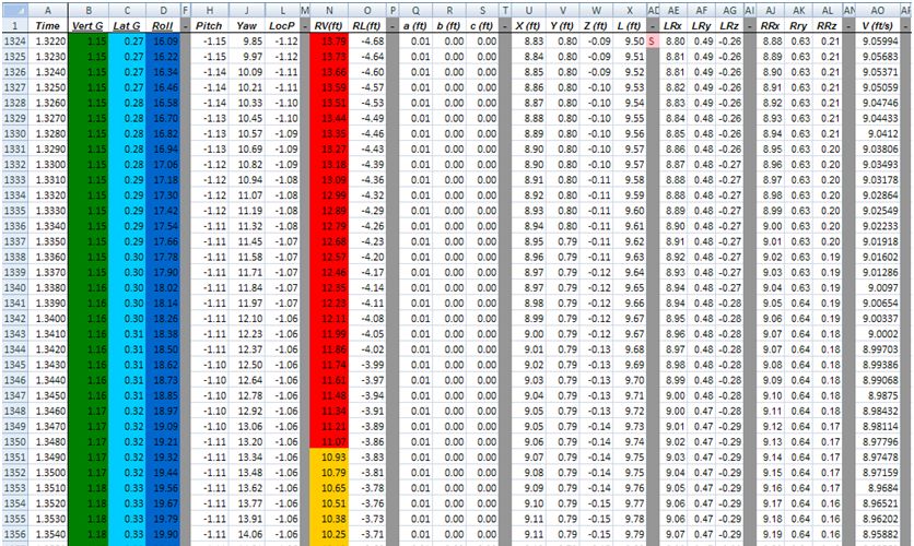
being initially stationary with respect to the car; while this may produce
some percentage of the g’s they experience, the majority of forces exerted
come from gravity and the phenomenon of centripetal acceleration. These
centripetal forces arise from the inherent curving nature of a roller coaster,
which can be described in its simplest terms as ever changing radii of curva-
ture. In two spatial dimensions, centripetal acceleration Ac is proportional to
the square of a moving object’s velocity v divided by the radius of curvature
R:
                                         v2
                                   Ac =                                   (2.1)
                                         R
    In three dimensions, the track’s curvature can be described in two or-
thogonal radii of curvature, the vertical radius and the horizontal radius.
The positive conventions of the radii are shown in Figure 2.1 where negative
vertical and horizontal radii would go down and to the left, respectively. It is
important to remember that these radii are with respect to the car’s current
spatial orientation; in the case that the car is completely on its side, the
vertical and horizontal radii are actually oriented horizontally and vertically,
respectively, with respect to a global coordinate system. As Equation 2.1
implies, no acceleration is achieved when a radius approaches infinity; this
makes logical sense, as a radius of infinity corresponds to straight track. A
radius revolving around an axes tangentially aligned with the car’s direc-
tion of travel is not needed for its centripetal effects are mostly negated by
something called heartlining, which will be discussed shortly.
    Yaw, Pitch, Roll, and Heartlining: Whereas the radii of curvature are
used to describe a car’s path of travel, yaw, pitch, and roll are used to
describe the direction the car is traveling in three dimensions. As shown in
Figure 2.2, yaw changes describe a rotation around an axis pointing up from
the car, pitch changes describe a rotation about an axes pointing out from
the car’s side, and roll changes describe a rotation about the axis tangentially
aligned with the car’s direction of travel. Thus, current total yaw, pitch, and
roll values with respect to a global set of axes can be used to fully describe
the car’s orientation.
    As mentioned before, a radius of curvature associated in the direction of
the roll is not needed because of heartlining. Heartlining is how the design
process takes into account the fact that the car is not a point mass (in
this project, it has dimensions of 4” wide, 3” high, and 6” long). What
is actually designed by the spreadsheet is the center “heartline”, or where

                                       3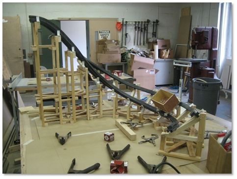
Figure 2.1: Radii of Curvature

the rider’s hearts would theoretically be as the car traverses the track; the
locations of the track’s rails are calculated by using an adjustable constant
offset distance from the heartline. All roll rotations are taken with respect
to the heartline, meaning that riders’ hearts are least subject to any residual
g-forces caused by rolling due to a minimized moment arm. While it is
impossible to have all riders in this middle position (due to capacity, cars
are multiple seats wide), the distances of each rider’s heart to the heartline
is small enough such that rolling effects are negligible. The length of a
Train (many cars grouped together) actually contributes more to any g-force
discrepancy because velocity at any given point of design is taken from the
heartline point of the middle car. Because the entire train must travel at the
same speed and yet each car must exist at a different point along the track
(most likely with slightly different radii of curvature), the g-forces are often

                                       4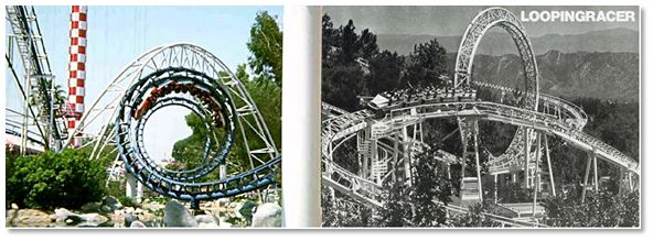
Figure 2.2: Yaw, Pitch, and Roll

varied through the train. Calculating just how different the g-forces are on
different cars of a train is a relatively easy problem to solve and will be shown
later, although because only one car was used in this project, it was not a
concern.
    Running, Guide, and Up-stop wheels: Modern day roller coasters utilize
complex wheel assemblies so that the cars cannot leave the track. The main
wheels of a roller coaster are simply referred to as running wheels. Guide
wheels are either on the insides or the outsides of the rails and constrain the
train from moving laterally with respect to the track. The upstop wheels are
on the bottom of the rails and ensure that the train cannot lift off.
   The car used in this project, depicted in Figure 2.3, has some leeway in
the space between the wheels. This is because of the relatively less accurate

                                       5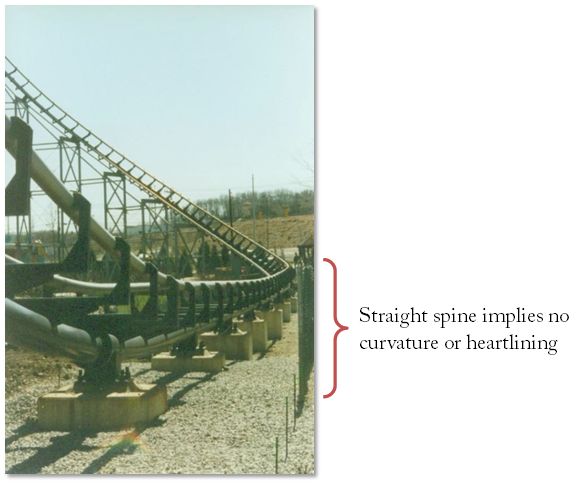
Figure 2.3: Wheel Assembly Constraining the Train to the Track

track curvature inherent with coasters where the track is fabricated on the
supports themselves (this mostly applies to wooden-tracked roller coasters,
as opposed to steel roller coasters where the track is entirely fabricated in a
factory) and to ensure that the car can navigate track curvature despite its
own rigidity.

2.2    History
    Now that the relevant terms have been covered, it is easier to understand
the evolution of the roller coaster and how this project fits within the larger
picture. Many sources attribute the beginning of the roller coaster to 17th
century Russian ice slides. Just like most modern day roller coasters, the ice
slides were completely gravity powered. The idea of a gravity powered cart
used to entertain riders eventually spread through Europe, most notably
France, who created the first slides that navigated wheeled-wooden carts
down their courses.

                                      6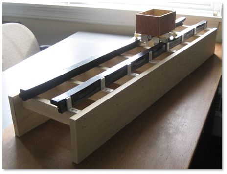
Figure 2.4: The French Take on the Russian Ice Slides

     The craze crossed the Atlantic and hit the US in the late 19th century
in the form of Switchback and Scenic Railways. These rides would become
the main attractions at amusement parks around the country, most of them
being situated near beaches and boardwalks. These primitive roller coasters
still did not attain the great heights and speeds that are commonplace today,
and thus g-forces were not much of a concern.
    Along with the new heights and speeds being sought after by amusement
park entrepreneurs, new elements were also being created. The vertical loop,
what has become one of the defining symbols for roller coasters, dates back
to the late 1800’s. The loops of these early inverting rides were not designed
with g-forces in mind and they were often dismantled due to discomfort; as
seen in Figure 2.5, the loops were too circular to account for the fact that
velocity was far greater at the bottom than at the top. Equation 2.1 shows us
that the forces associated with the centripetal accelerations would vary even
more than the velocities at those different heights. The way that primitive
loops were shaped strongly suggests that roller coaster designers at the time
were more concerned with designing a ride that could complete a full circuit
than designing a ride to utilize g-forces to enhance the ride experience, let
alone for safety concerns.
   The 1920’s corresponded with what is known as the First Golden Age

                                      7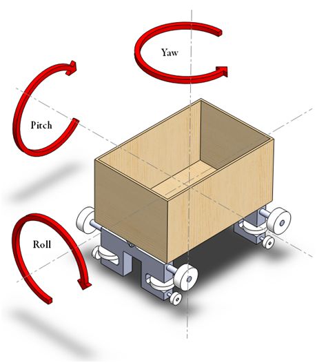
Figure 2.5: An Early Prototype of a Looping Coaster

of Roller Coasters. It was during this time that such legendary classics like
the Thunderbolt at Kennywood in Pittsburgh, the Giant Dipper at Santa
Cruz Beach Boardwalk, and the Coney Island Cyclone in Brooklyn were
built. What is often referred to as the most intense roller coaster at the time
was the Crystal Beach Cyclone, designed by Harry Traver. Traver’s rides
pushed the envelope far more than any others (some had to have nurses at
their exits, just in case), and it is almost unfortunate to think that if he had
the knowledge that the industry currently has about g-forces and safety in
general, more of his designs would still be standing today.
    As the economy took a turn for the worse at the end of the 20’s, roller
coaster construction and innovation essentially came to a halt. Interest in
roller coasters picked back up with the opening of Disneyland’s Matterhorn
Bobsleds in 1959. The Matterhorn was the first coaster to use tubular steel
track, what all modern day steel roller coasters are based on today. Because of
the added track accuracy associated with prefabrication and stronger support
structures, steel roller coasters could be built taller, faster, and with much
more complex track curvatures. Corkscrew at Knott’s Berry Farm and The
Revolution at Magic Mountain represented the first modern inverting roller
coasters when they opened in 1975 and 1976, respectively. While these rides
were better designed to keep g-forces in check, they still paled in comparison
to today’s roller coasters in their design precision.
   The limits of g-forces were pushed to their limits in the 1980’s, led by
famed German designer Anton Schwarzkopf (designer of the Revolution).
The Thriller, which was designed as a looping, traveling steel coaster that

                                       8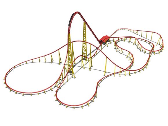
Figure 2.6: The Corkscrew (Left) and the Revolution (Right)

made its way throughout Germany, attained the highest (vertical) g-force
rating on a roller coaster ever at 6.7. The ride had since been modified to
reduce that number, yet still its intensity has caused it to be dismantled from
two Six Flags parks before finding its current home in Mexico in 2008.
    The addition of inversions to roller coasters necessitated new restraints.
The downside to these new “over-the-shoulder-restraints” (otsr’s) was that
lateral g’s would bang riders’ heads against the restraints, causing great
discomfort. It is this reason as to why steel roller coasters are not designed
to induce lateral g’s like their wooden, lap-bar restrained counterparts are.
Even though turns were banked appropriately to balance out gravitational
forces and centripetal forces to produce zero net lateral g’s, the banking
transitions were overlooked. Banking transitions, notably those designed by
Arrow Dynamics, Vekoma Rides Manufacturing, Schwarzkopf, and Intamin
AG were designed in a straight line and were not heartlined.
    The banking transition in Figure 2.7 is completely straight, and in the
absence of any horizontal radius of curvature, the train will experience un-
wanted lateral g’s just due to gravity (this will be shown mathematically
later). Thus we can see that in rides during this period, as recent as the
mid 1990’s, the g-forces were not kept under close supervision at all times
during ride duration. One can also see in the figure that the roll’s center of
rotation is the track’s spine (i.e. not heartlined) and so the eccentricities that
the riders had with respect to the center of rotation added to the unwanted
g’s and thus increased rider discomfort.

                                        9
Figure 2.7: Straight Banking Transition on Kennywood’s Steel Phantom
A solution to removing lateral g-forces from a banking transition is to
induce corresponding lateral g’s in the opposite direction that cancel out the
effects of gravity. This can be easily accomplished by giving the track a
horizontal radius of curvature, in essence making the track ease into or out
of the turn gradually even before the transition is completed to ensure that
unwanted lateral g’s are not ever experienced.
As designers evolved towards the end of the 20th century to the present
day, it is clear that a lot more emphasis has been placed on g-forces being
an integral part of the ride. Positive vertical g-forces are often advertised
for modern roller coasters, signifying how powerful they can be. Negative
vertical g-forces are lauded by roller coaster enthusiasts, who have christened
them as “Airtime”. Lateral g-forces on wooden coasters, where the restraint
system is always more or less some derivative of the simple lap bar, give these
rides a sense of being out of control. g-forces can be used to tell a story,
and designers are getting better and better at creating interesting plotlines.
The recently opened Intimidator 305 ™ at Kings Dominion uses vertical g-
10forces to its benefit almost more than any other ride. It cleverly integrates
longer durations of gentler airtime, quick moments of intense airtime, big
helpings of strong positive g’s, and even banking transitions that are taken
so quickly that the airtime is produced from the centripetal force (arising
from the radius of curvature I previously said was negligible!) in a ride that
the manufacturer president calls “... a rider’s ride and is the most aggressive
we have done to date.”1
Figure 2.8: “Intimidator 305™” at King’s Dominion, Opened 4/1/10
1
News Plus Notes, http://newsplusnotes.blogspot.com
113 Design Process
3.1 Equations of Equilibrium
The heart of the design is focused around the free body diagram (FBD).
The FBD allows the design of the coordinates and angles of the track in ac-
cordance with g-forces. The design process iterates over intervals of one mil-
lisecond, updating the FBD each time as roll, pitch, and yaw angles change,
to calculate the next iteration’s coordinates and orientation based on g-forces.
As shown in Figure 3.1, the “rider” centered FBD has a global coordinate
axes labeled X, Y, and Z (with X pointing into the page) while the corre-
sponding local axes are labeled a, b, and c (a in this case is aligned with X).
Note that the roll angle φ is depicted in the figure while the pitch angle θ
and the yaw angle ψ could not be illustrated in this view.
Figure 3.1: Free Body Diagram; Car is Going Into the Page
With the FBD in place, it makes sense to then derive equations for vertical
and horizontal radii of curvature and, in turn, use these to calculate the
12next point’s coordinates described by the current local coordinate system.
In Equation 3.1, the radii are denoted by R and the g-forces by G while
the subscripts V and L denote vertical and horizontal (lateral) directions,
respectively. α and β will be explained shortly.
2
v2
v
m +g∗β = m(GV ∗ g) =⇒ RV =
RV g(GV − β)
2
v2
v
m +g∗α = m(GL ∗ g) =⇒ RL = (3.1)
RL g(GL − α)
The local change in coordinates can be calculated once the radii of cur-
vature are determined. A displacement in the train’s forward direction, a,
is calculated by multiplying the velocity by a specified time interval. Using
equations describing the path of a circle, values for the local displacements b
and c can be calculated. In Figure 3.2, which shows the local displacements
for a positive vertical radius of curvature, it is obvious to see that the car will
not follow the path of a true circle if a is chosen to be too large. The small
time interval chosen ensures that this does not occur, i.e. this approximation
becomes a perfect circle as a tends to zero.
Figure 3.2: a and b; Diagram for a and c is Analogous
13q
a2 + (b − RV )2 = RV2 =⇒ b = RV ± RV2 − a2
q
a2 + (c − RL )2 = RL2 =⇒ c = RL ± RL2 − a2 (3.2)
In Equation 3.2, the train is set to be on the path of the circle rather than
its center by subtracting the radius value from the orthogonal displacement
on the left hand side. The sign in front of the radical chosen on the right
hand side is the opposite of the sign of the radius in order to make sense
geometrically.
3.2 Local to Global Displacements
Once these new coordinates are found, they can be translated into a
global frame by means of a transformation array, shown in Table 1, in order
to monitor where the track is. The global coordinates are essentially what
our end goal is, the part of the spreadsheet that can be used to construct the
track (after heartlining offsets are taken into consideration).
X Y Z
a cos θ ∗ cos ψ − sin φ ∗ sin ψ − cos φ ∗ cos ψ ∗ sin θ cos φ ∗ sin ψ − cos ψ ∗ sin θ ∗ sin φ
b sin θ cos θ ∗ cos φ (= α) cos θ ∗ sin φ (= β)
c − cos θ ∗ sin ψ cos φ ∗ sin θ ∗ sin ψ − cos ψ ∗ sin φ cos φ ∗ cos ψ + sin θ ∗ sin φ ∗ sin ψ
Table 1: 3D Transformation Array
It is important to consider the order of operations when converting co-
ordinates. For example, the above three-dimensional array was computed
by multiplying together (by matrix multiplication) the transposes for two-
dimensional arrays for yaw, pitch, and roll in that order; the array produced
actually works for changes of orientation in the opposite order, which is the
order that the design process utilizes. Because gravity acts in the (negative)
global Y direction, the α and β in the 3D transformation array represent the
term in the second row, third column and second row, second column, respec-
tively; the effects of gravity have to be converted into the local coordinate
system before the (local) radii of curvature can be calculated.
14Figure 3.3: Relating Local Axes to Global Axes
To further clarify the use of the transformation array, the simplified,
analogous case is illustrated in Figure 3.3. For a displacement of distance a
in the a direction, geometry lets us describe this in the global frame as a∗cos θ
in the X direction plus a∗sin θ in the Y direction. Likewise, displacement b in
the b direction can be described as −b ∗ sin θ in the X direction and b ∗ cos θ
in the Y direction. Table 2 reflects this: the total displacement in the X
direction is found by adding together all the products of the displacements
at the beginning of each row and their corresponding term in the X column.
This is the same method used with the 3D array.
X Y
a cos θ sin θ
b − sin θ cos θ
Table 2: 2D Transformation Array
3.3 Calculating Yaw and Pitch
The new pitch and yaw values are calculated based on the local changes
in pitch and yaw, which are in turn calculated by seeing how far along the
radii of curvature the car has gone in the time step. An arc length in any
circle can be calculated by multiplying the change in angle by the radius,
and so approximating the arc length to be the straight line distance from the
initial point to the final point, the local change in pitch (and yaw) can be
found. Because the two radii are orthogonal, the global change in pitch and
15yaw can be calculated by adding the correct proportions of the local changes.
√ √
a2 + b 2 a2 + c 2
∆θlocal = ∆ψlocal =
RV RL
∆θglobal = ∆θlocal ∗ cos φ + ∆ψlocal ∗ sin φ
∆ψglobal = ∆θlocal ∗ sin φ − ∆ψlocal ∗ cos φ/ cos θ (3.3)
The equation for global change in yaw differs slightly from the global
change in pitch because the local change in yaw has to be adjusted to isolate
the component in the global X-Z plane.
4 The Spreadsheet
4.1 Implementation
A sample of the spreadsheet can be found in Figure 4.4. The default
process of the spreadsheet is to input the vertical and lateral g-forces as well
as the desired roll angle, and using the equations derived in the last section,
the radii of curvature, the local and global displacements, and updated ve-
locity can be calculated in that order. The spreadsheet calculates the rail
locations by converting specified offset distances into global displacements
from the heartline using the transformation array. Velocity is calculated by
having the user input friction coefficients for the running and guide wheels
(it can be adjusted to incorporate upstop wheel friction, but in practice this
value was the same as it was for the running wheels so there was no need
to differentiate between the two) tat are used in conjunction with a simple
physics equation to find the frictional loss of the car as a function of the
distance it has traveled and its orientation. After showing my constructed
train to Professor Nelson Macken, we concluded that the drag on the car will
be negligible such that using an additional term involving the square of ve-
locity would not be necessary. Thus, while it has been understood that much
more complicated models exist for this calculation, the simple notion that
the dry friction (coefficient µ multiplies normal force) of the ball bearings
would govern velocity losses was used.
Note that when a radius of curvature exists, the normal force in Figure 4.1
will not equal mg ∗ sin θ. In fact, the normal force will always be the amount
16Figure 4.1: Friction FBD
g’s multiplied by the mass, and this is reflected in the following equations.
The angle in the FBD is the negative of θ because pitch is measured positive
when the car is tilted upwards; this is accounted for as well in Equation 4.1
(simplified for non-inverting track).
vf2 = v02 + 2 ∗ Acceleration ∗ ∆distance
1
Acceleration = (mg ∗ sin(−θ) − µ ∗ Fn )
q m
=⇒ vf = v02 + 2[g(− sin θ − [µv ∗ Gv + µl ∗ Gl ]) ∗ ∆distance] (4.1)
Referring back to Figure 2.3, the leeway between the wheels and track
ensure that the running and upstop wheels are never in contact with the
track concurrently (nor are both guide wheels), thus accounting for the what
was substituted for µ ∗ Fn .
174.2 g-force Transitions
It is important to note that the inputs for the spreadsheet are not in-
cremented suddenly as if they were step functions. For example, suddenly
changing from 1 g in the vertical direction to 3 g’s in 1 millisecond would
frankly be painful for riders. The transition from an initial value to a final
value is done usually with either a 5th degree or 4th degree polynomial in
order to ease riders into the final g value. These polynomials can be nor-
malized for duration and amplitude as necessary, making use of the discrete
time column in the spreadsheet. It is also possible to have these polynomials
change values in multiple columns at the same time, which produces an in-
teresting flow of g-forces and other values that may not be conceivable when
designing with more conventional methods. Other types of polynomials can
be used as well, including ones that dip down to a certain value before grad-
ually increasing back to its initial value or ones that oscillate multiple times
during their durations.
Figure 4.2: 5th and 4th Order Polynomials Used
184.3 g-force Discrepancies
In Section 2.1, the problem of varying g-forces throughout a train of linked
cars was discussed. The spreadsheet can easily calculate what the forces are
along the train once the coordinates and angles are set. Because each car
in the train must have the same velocity at any given time, g-force curves
for any car can be calculated by using the length column (labeled X) to see
how many rows account for the length between the car in question and the
center car, and then shifting the velocity column AO by that amount while
reconfiguring the equations of g-forces to be calculated from the velocity and
track geometry. For extremely wide cars (the Griffon at Busch Gardens
Europe seats 10 riders across in three-car trains), a similar method can be
used to calculate g-forces at any seat. A specified offset can be used to find
the exact path of a seat in a similar fashion to how the rail locations are found,
and the equations could then be reworked to solve for local displacements
and radii of curvature, the seat’s velocity, and finally g-forces.
4.4 Visualization
While 2D plots are kept in Excel in order to better visualize the design,
a program that I created in Matlab takes in the spreadsheet, extracts the
necessary columns, and plots the track in 3D. Ties between the rails are also
plotted signifying where supports will be dictating the track’s orientation,
explained later in Figure 5.4. The code for this program can be found in the
Appendix.
As a side note, the element pictured in Figure 4.3 is what the industry
calls a “zero-g” roll for riders revolve in a full barrel roll while experiencing 0
g’s. The black line represents the heartline, and with this element, it is easy
to see how the heartline is the center of roll rotation. I plan to continue using
the spreadsheet to design roller coasters in the styles of real manufacturers
(without actually building the track itself). The goal in this is to show that
my spreadsheet could represent the foundation for a design process applicable
to the industry.
1920
Figure 4.3: 3D Plot of a Designed Track Element21
Figure 4.4: The Design Spreadsheet5 Construction
5.1 Determining Friction
The wheel assemblies and cabin that make up the car were designed in
SolidWorks and constructed in the machine shop during the Fall semester.
What was not shown in these Figure 2.3 was a foam substance between
the wheel assemblies that act in the same manner as suspension acts on
automobiles. This was done so that the front assembly and the rear assembly
did not have to always be aligned, enabling the car to navigate tighter track
twists. Ball bearings were inserted into each of the car’s 12 wheels. A 3.5’
long, straight test track was also built to both determine the best methods
to construct the track as well as for straight-line friction testing.
Figure 5.1: Straight Test Track and Car
A Freescale MMA7456L tri-axis accelerometer with ZStar3 wireless tech-
nology was purchased to both analyze the friction and measure the g-forces
acting on the car on (future) curved tracks. The only modification that had
to be made before the accelerometer could be used was that its power saving
algorithm had to be disabled. After contacting the manufacturer, this was
22done simply by removing an “if” statement in the code and then synchro-
nizing programs with the accelerometer using a Background Debug Mode
(BDM) Multilink. Once this was done, the accelerometer did not skip any
data points in efforts to prolong battery life as it had been initially pro-
grammed to do.
Friction data was taken by aligning the proper accelerometer axes with
the car’s and then simply nudging the car down the straight track, letting its
own friction force it to a halt. Many trials of this were done with the car riding
on top of the track as well as orienting the track on its side to see the friction
effects from the guide wheels and upside down to see the friction effects from
the upstop wheels. While in upright orientation, the car was also loaded with
an assortment of weights to see if there was added friction when simulating
added g-forces on the bearings. The friction data was automatically uploaded
into Microsoft Excel by the accelerometer’s computer graphical user interface.
Once in Excel, the data had to be slightly adjusted for error. This was
done by numerically integrating the acceleration data in the forward direction
to obtain velocity, and a small constant was subtracted from all velocity data
points until the velocity showed as declining to zero at the end of the trial.
As an extra precaution, the velocity data was integrated as well to obtain
displacement, and the final distance traveled of roughly 2’ was also verified.
Friction values were obtained by creating a linear fit with the velocity curves,
which yielded promising R2 determination coefficients ranging from .972 to
.995.
Figure 5.2: Friction Graph after Numerical Integration and Correction
23Acceleration Data (g)
Trial 1g 2.32g 4.27g 8.61g Side UD (-1g)
1 .033043 .03059 .034006 .035 .042609 .051025
2 .035839 .011273 .010093 .033075 .03723 .044522
3 .034255 .031025 .042422 .041242 .03723 .044522
4 .054969 .047857 .049907
5 .033106 .043447
Table 3: Friction Data for Upright, Side, and Upside Down
As seen in Table 3, there did not seem to be a linear relationship between
friction experienced and simulated g-force. I strongly suspect that this had
something to do with the acceleration readings being on the order of magni-
tude of the noise read by the accelerometer while the car was idle. Regardless,
the data did seem relatively consistent and so as a starting point to input
into the spreadsheet, I used conservative values of .06 for vertical dry friction
(µ value) and .05 for lateral. In reality, roller coasters are designed conser-
vatively due to the fact that energy from gravity is a lot easier to get than
energy by some mechanical boosting system; if the train tested too quickly
through certain elements as to reduce rider comfort or safety, a “trim brake”
is usually installed on the track to bring the train back down closer to its
predicted velocity. If friction values were underestimated, the train may not
have enough energy to navigate the course. Again, it is important to note
that a more complex friction model, i.e. one that incorporated air drag and
thus losses proportional to the square of velocity, was not used. This could
account for any error that arose during tests.
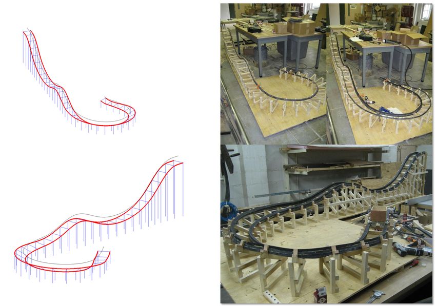
5.2 Test Tracks
Both the first and second curved test tracks were built similarly to real
wooden coasters in that the track itself was fabricated on the structure rather
than being prefabricated; the structure dictates the track curvature as well
as supports the track. The test track structures were built by connecting
precisely assembled bents, the elements of the structure consisting of vertical
members, to a large piece of plywood. The track was then created by stapling
24Figure 5.3: First Curved Test Track
a layer of rubber to wooden angles on top of the bents; this was done so that
if needed, the track could be adjusted as the angles had slots in them where
a single screw secured them. More layers of rubber were attached on top of
the bottom layer with panel adhesive, and this gave the track a very rigid
yet accurately curved shape.
An arbitrary value of 6” of track between bents was implemented into the
3D rendering code in order to view how different the actual track coordinates
could be with respect to the design; in Figure 5.4, one can see the difference
between the designed rail locations and what the rail locations would be if
the track was fabricated as 6” straight lines between the bents (the curve
above the track is the heartline). The fact that the rails are so similar to one
another confirms that 6” was a good bent separation distance.
The second test track design itself was roughly 2.5’ tall and roughly 18’
long. It was designed primarily by inputting the g-forces and refining them
until the desired curves were attained; in a sense, the design process was
iterative both in the trial and error (associated with much of engineering
design in general) as it was iterating over thousandths of a second to get
25Figure 5.4: Possible Track Error
as close to true arcs as possible. The last portion of the ride, consisting of
the 30 degree flat banked turn, was designed by first inputting the desired
lateral g and roll curves, then setting the vertical radius of curvature equal
to the horizontal radius divided by the tangent of the roll, and then calcu-
lating vertical g’s based on the vertical radius to ensure they were still safe.
The bigger picture here is that the spreadsheet can be fully manipulated to
meet certain demands just by rearranging the equations of equilibrium. The
downward helix in Figure 7.1, for example, was made by first locking in the
coordinates for the heartline as to minimize wooden structure complexity
with the overlapping track and then setting up the spreadsheet to adjust the
roll to give linearly increasing lateral g’s all the way down, freeing riders of
its grip right before it was too much to handle.
6 Data Analysis
In a similar fashion to the friction tests, the accelerometer was attached
to the car and tests were performed. As predicted after seeing the train run
through the previous test track, friction was a lot higher than anticipated.
This was due to rail misalignment, mostly during the banked turn, as the
softness of the rubber disallowed for more precise fabrication. After seeing
this both qualitatively and quantitatively, I rearranged the spreadsheet so
that the g’s could be analyzed at higher friction values. The rubber track
was then replaced with harder rubber, and the tests were run again.
26Figure 5.5: Rendering and Construction of Final Test Track
Figure 6.1 and Figure 6.2 show how the actual data compared with the
initial predictions. In Figure 6.3 and Figure 6.4, one can see that there was
much more noise in the lateral g-force graph compared to the vertical g-force
graph because there was leeway between the guide wheels and the track,
allowing the car to shift slightly side to side in order to ensure that the rails
do not squeeze in on the wheels. This is often experienced in real wooden
roller coasters for the same exact reason. Also note that the data from the
harder rubber better matched the initial predictions as one would expect.
Figure 6.3 shows how the friction-adjusted data corresponded with the
27Figure 6.1: Vertical g Predictions and Actual Data
Figure 6.2: Lateral g Predictions and Actual Data
28Figure 6.3: Initial Friction Adjustments to Match Initial Track Data
Figure 6.4: Final Friction Adjustments to Match Initial Track Data
29data from the initial, soft rubber track. Friction was adjusted until the
highest R2 values (one coefficient of determination for vertical g-force and
one for lateral) were obtained. In Figure 6.4, the highest R2 values were
obtained at lower friction values than those used to match the data from
the track with less rigid rubber as expected. The values in Table 4 below
were calculated from a function I wrote in Matlab that can be found in the
Appendix.
R2 Coefficients of Determination
Initial Predicted Data Initial Adjusted Data Final Adjusted Data
Vertical Lateral Vertical Lateral Vertical Lateral
Initial Data -1.1390 -6.8201 .8411 .3561 n/a n/a
Final Data .3226 .1854 n/a n/a .9481 .8800
Table 4: R2 Coefficients of Determination
As shown in Table 4, the initial predictions were indeed closer to the final
track than they were to the initial, softer track. The negative values correlat-
ing the initial predictions with the initial track signify very bad correlations;
while the common misconception is that R2 values have a range of 0 to 1, I
confirmed in Matlab that the value can be negative for very bad fits. While
the coefficients relating the first adjusted values to the initial track data had
comparatively decent coefficients of determination, the coefficients between
the final adjusted values and final track data were noticeably superior and
show great promise for the validity of this design process. The coefficients
for all the lateral g-force data were all lower than their vertical counterparts,
as expected, due to the shifting that was alluded to earlier.
7 Conclusion
While the final track data and the spreadsheet differed noticeably, I was
able to show that the spreadsheet did in fact work by producing much more
accurate curves once friction values were adjusted. This confirmed my sus-
picions when conducting friction tests; seeing that the friction values read
by the accelerometer were comparable to the noise produced when it was
not moving, doubts were raised as to the validity of the friction coefficients
30obtained from the tests. Track fabrication seems to have been the biggest
cause of velocity loss on my final track, but if anything, this mimics the track
fabrication non-idealities associated with real wooden coasters relative to the
rigidity of their cars. Wooden coasters constantly have to be re-tracked in
order to ride relatively smooth, and even then they are never as smooth as
their steel, prefabricated track counterparts (although many argue this is a
good thing). Very recent wooden coaster technology has sought to address
these problems, including the Gravity Group creating their new, more flex-
ible “Timberliner” trains, Great Coasters International retrofitting some of
their older coasters with their more flexible “Millennium Flyer” trains, and
companies like Intamin AG designing with prefabricate wooden track to be
literally “plugged in” to its wooden support structure. Six Flags over Texas
is currently retrofitting the wooden coaster the “Texas Giant” with prefab-
ricated steel rails; while this will improve the smoothness of the ride, roller
coaster enthusiasts are worried that the ride will cease to feel like a wooden
coaster.
A roller coaster has to be designed in the face of non-idealities. So many
variables have to be taken into account so that the ride can run in various
conditions, ranging from different wind speeds, heterogeneous distribution of
riders’ weights, or even birds that may be nesting on the track. The best
roller coaster is one that can offer a thrilling experience while being able to
operate under all these conditions.
Pictured in Figure 7.1 are the beginnings of my own design, incorporating
many elements that pay homage to great coasters that I have ridden as well
as new ideas I have thought up on my own. A main goal of the design was to
be able to have a short (roughly 40’ tall) ride be able to produce the g-forces
found on much larger tracks, and the figure above along with the apparent
strength of my spreadsheet shows that this is definitely possible. The ride’s
name is “David”, a name that plays on how David held his own against Go-
liath (coincidentally, other large, real coasters are named “Goliath”), how
during my education, Swarthmore has held its own against large universi-
ties, and how my father David continues to be an inspiration to me. The
philosophy of this design’s layout is discussed in a separate paper.
Through this project and through my four years at college, one of the
many things I have learned is that I still do in fact want to design roller
coasters, even though now I know a lot more about what that entails.
31Figure 7.1: “David”, My Own Wooden Track Design. Dots represent
the car’s location at every tenth of a second.
8 Acknowledgments
• Professor Cheever for his help in advising this project
• Professors Macken and Siddiqui for their advice
• Keith Cohn, whom I met at the Coaster Crazy message boards
(http://www.coastercrazy.com/) for his help with the equations of equi-
librium
• Grant “Smitty” Smith and Steve Palmer for their help in constructing
the tracks
• Freescale Semiconductor (http://www.freescale.com/) for their excel-
lent customer service regarding modifying the accelerometer’s program-
ming
• Bennett, David. Roller Coaster: Wooden and Steel Coasters, Twisters,
and Corkscrews. Edison, N.J.: Chartwell, 1998. Print. (Figure 2.5)
• Coker, Robert. Roller Coasters: a Thrill Seeker’s Guide to the Ultimate
Scream Machines. New York: Barnes Noble, 2003. Print. (Figure 2.4)
• For images used in this paper:
32– Coaster-Net (coaster-net.com) (Figure 2.6, Right)
– Encyclopedia Britannica (www.britannica.com) (Figure 2.6, Left)
– Kings Dominion (www.kingsdominion.com) (Figure 2.8)
– Roller Coaster Database (www.rcdb.com) (Figure 2.7)
• Erik Smith and Rachel Adler for their help in writing this report in
LATEX 2ε
• Other friends and family who have helped out in various ways during
the year
33A Matlab Functions to Plot Track and to Cal-
culate R2
1 function plotTrack4(data,tieSpace)
2 %Plots the track
3 %Inputs are data matrix and tie spacing in feet
4
5
6 %Number of points
7 num = ceil(max(data(:,29))/tieSpace);
8
9 %Initializing Rail Coordinate Vectors
10 z=zeros(num,4);
11 x=z;
12 y=z;
13
14 %Filling in Rail Coordinates
15 z(1,1)=data(1,33);z(1,2)=z(1,1);z(1,3)=data(1,38);z(1,4)=z(1,3);
16 x(1,1)=data(1,31);x(1,2)=x(1,1);x(1,3)=data(1,36);x(1,4)=x(1,3);
17 y(1,2)=data(1,32);y(1,3)=data(1,37);
18 for i=2:length(data)
19 if mod(data(i,29),tieSpace)41 plot3(z(i,:),x(i,:),y(i,:),'b')
42 end
43
44 %Adjust Axes
45 xlabel('Z'),ylabel('X'),zlabel('Y')
46 d=min(min([min(data(:,23)) min(data(:,21)) min(data(:,22))
47 min(data(:,33)) min(data(:,31)) min(data(:,32))
48 min(data(:,38)) min(data(:,36)) min(data(:,37))]));
49 e=max(max([max(data(:,23)) max(data(:,21)) max(data(:,22)),
50 max(data(:,33)) max(data(:,31)) max(data(:,32)),
51 max(data(:,38)) max(data(:,36)) max(data(:,37))]));
52 axis([d e d e d e])
1 function rSquared(predictedData,actualData,column)
2 %Finds the Coefficient of Determination (rˆ2) for two data sets
3
4 ssTot=0;
5 ssErr=0;
6 ssReg=0;
7 yBar=mean(actualData(:,column));
8 for i=1:length(actualData)
9 ssTot=ssTot+(actualData(i,column)-yBar)ˆ2;
10 for j=1:length(predictedData)
11 if abs(actualData(i,1)-predictedData(j,1))You can also read