CHAOS Challenge - Combined (CT-MR) Healthy Abdominal Organ Segmentation - Combined (CT-MR) Healthy Abdominal ...
←
→
Page content transcription
If your browser does not render page correctly, please read the page content below
CHAOS Challenge - Combined (CT-MR) Healthy
                             Abdominal Organ Segmentation
                             A. Emre Kavura,∗, N. Sinem Gezerb , Mustafa Barışb , Sinem Aslanc,d , Pierre-Henri Conzee , Vladimir Grozaf , Duc Duy Phamg ,
                             Soumick Chatterjeeh,i , Philipp Ernsth , Savaş Özkanj , Bora Baydarj , Dmitry Lachinovk , Shuo Hanl , Josef Paulig , Fabian Isenseem ,
                             Matthias Perkoniggn , Rachana Sathisho , Ronnie Rajanp , Debdoot Sheeto , Gurbandurdy Dovletovg , Oliver Specki , Andreas
                             Nürnbergerh , Klaus H. Maier-Heinm , Gözde Bozdağı Akarj , Gözde Ünalq , Oğuz Dicleb , M. Alper Selverr,∗∗
arXiv:2001.06535v2 [eess.IV] 9 May 2020

                             a Graduate   School of Natural and Applied Sciences, Dokuz Eylul University, Izmir, Turkey
                             b Department   of Radiology, Faculty Of Medicine, Dokuz Eylul University, Izmir, Turkey
                             c Ca’ Foscari University of Venice, ECLT and DAIS, Venice, Italy
                             d Ege University, International Computer Institute, Izmir, Turkey
                             e IMT Atlantique, LaTIM UMR 1101, Brest, France
                             f Median Technologies, Valbonne, France
                             g Intelligent Systems, Faculty of Engineering, University of Duisburg-Essen, Germany
                             h Data and Knowledge Engineering Group, Otto von Guericke University, Magdeburg, Germany
                             i Magnetic Resonance, Otto von Guericke University Magdeburg, Germany.
                             j Department of Electrical and Electronics Engineering, Middle East Technical University, Ankara, Turkey
                             k Department of Ophthalmology and Optometry, Medical Uni. of Vienna, Austria
                             l Johns Hopkins University, Baltimore, USA
                             m Division of Medical Image Computing, German Cancer Research Center, Heidelberg, Germany
                             n CIR Lab Dept of Biomedical Imaging and Image-guided Therapy Medical Uni. of Vienna, Austria
                             o Department of Electrical Engineering, Indian Institute of Technology, Kharagpur, India
                             p School of Medical Science and Technology, Indian Institute of Technology, Kharagpur, India
                             q Department of Computer Engineering, İstanbul Technical University, İstanbul, Turkey
                             r Department of Electrical and Electronics Engineering, Dokuz Eylul University, Izmir, Turkey

                             Abstract
                             Segmentation of abdominal organs has been a comprehensive, yet unresolved, research field for many years. In the last decade, intensive de-
                             velopments in deep learning (DL) have introduced new state-of-the-art segmentation systems. Despite outperforming the overall accuracy of
                             existing systems, the effects of DL model properties and parameters on the performance are hard to interpret. This makes comparative analy-
                             sis a necessary tool to achieve explainable studies and systems. Moreover, the performance of DL for emerging learning approaches such as
                             cross-modality and multi-modal semantic segmentation tasks has been rarely discussed. In order to expand the knowledge on these topics, the
                             CHAOS – Combined (CT-MR) Healthy Abdominal Organ Segmentation challenge has been organized in conjunction with IEEE International
                             Symposium on Biomedical Imaging (ISBI), 2019, in Venice, Italy. Healthy abdomen organ segmentation from routine acquisitions plays a signifi-
                             cant role in several clinical applications, such as pre-surgical planning for organ donation or size and shape follow-ups for various diseases. These
                             applications require certain level of performance on a diverse set of metrics such as maximum symmetric surface distance (MSSD) to determine
                             surgical error-margin or overlap errors. Previous abdomen related challenges are mainly focused on tumor/lesion detection and/or classification
                             with a single modality. Conversely, CHAOS provides both abdominal CT and MR data from healthy subjects for single and multiple abdominal
                             organ segmentation. Five different but complementary tasks have been designed to analyze the capabilities of current approaches from multiple
                             perspectives. The results are investigated thoroughly, compared with manual annotations and interactive methods. The analysis shows that the
                             performance of DL models for single modality (CT / MR) can show reliable volumetric analysis performance (DICE: 0.98 ± 0.00 / 0.95 ± 0.01)
                             but the best MSSD performance remain limited (21.89 ± 13.94 / 20.85 ± 10.63 mm). The performances of participating models decrease signif-
                             icantly for cross-modality tasks for the liver (DICE: 0.88 ± 0.15 MSSD: 36.33 ± 21.97 mm) and all organs (DICE: 0.85 ± 0.21 MSSD: 33.17
                             ± 38.93 mm). Despite contrary examples on different applications, multi-tasking DL models designed to segment all organs seem to perform
                             worse compared to organ-specific ones (performance drop around 5%). Nevertheless, some of the successful models perform better with their
                             multi-organ versions. Besides, such directions of further research for developing effective algorithms for cross-modality segmentation would
                             significantly support real-world clinical applications. Moreover, having more than 1500 participants, another important contribution of the paper
                             is the analysis on shortcomings of challenge organizations such as the effects of multiple submissions and peeking phenomena.

                                          ∗ Corresponding    author: e-mail: emrekavur@gmail.com
                                          ∗∗ Corresponding   author: e-mail: alper.selver@deu.edu.tr
2
1. Introduction domen. The remarkable developments in MRI technology in
terms of resolution, dynamic range, and speed enable joint anal-
In the last decade, medical imaging and image processing yses of these modalities (Hirokawa et al., 2008).
benchmarks have become effective venues to compare perfor- To gauge the current state-of-the-art in automated abdomi-
mances of different approaches in clinically important tasks nal segmentation and observe the performance of various ap-
(Ayache and Duncan, 2016). These benchmarks have gained proaches on different tasks such as cross-modality learning and
a particularly important role in the analysis of learning-based multi-modal segmentation, we organized the Combined (CT-
systems by enabling the use of common datasets for training MR) Healthy Abdominal Organ Segmentation (CHAOS) chal-
and testing (Simpson et al., 2019). Challenges, which use these lenge in conjunction with the IEEE International Symposium
benchmarks, bear a prominent role in reporting outcomes of the on Biomedical Imaging (ISBI) in 2019. For this purpose, we
state-of-the-art results in a structured way (Kozubek, 2016). In prepared and made available a unique dataset of CT and MR
this respect, the benchmarks establish standard datasets, evalu- scans from unpaired abdominal image series. A consensus-
ation strategies, fusion possibilities (e.g. ensembles), and (un- based multiple expert annotation strategy was used to generate
)resolved difficulties related to the specific biomedical image ground truths. A subset of this dataset was provided to the par-
processing task(s) being tested (Menze et al., 2014). An exten- ticipants for training, and the remaining images were used to
sive website, grand-challenge.org (van Ginneken and Kerkstra, test performance against the (hidden) manual delineations us-
2015), has been designed for hosting the challenges related to ing various metrics. In this paper, we report both setup and the
medical image segmentation and currently includes around 200 results of this CHAOS benchmark as well as its outcomes.
challenges. The rest of the paper is organized as follows. A review of the
A comprehensive exploration of biomedical image analysis current challenges in abdominal organ segmentation is given in
challenges reveals that the construction of datasets, inter- and Section II together with surveys on benchmark methods. Next,
intra- observer variations for ground truth generation as well CHAOS datasets, setup, ground truth generation, and employed
as evaluation criteria might prevent establishing the true poten- tasks are presented in Section III. Section IV describes the eval-
tial of such events (Reinke et al., 2018b). Suggestions, caveats, uation strategy. Then, participating methods are comparatively
and roadmaps are being provided by reviews (Maier-Hein et al., summarized in Section V. Section VI presents the results, and
2018; Reinke et al., 2018a) to improve the challenges. Section VII provides discussion and concludes the paper.
Considering the dominance of machine learning (ML) ap-
proaches, two main points are continuously being emphasized:
1) recognition of current roadblocks in applying ML to med- 2. Related Work
ical imaging, 2) increasing the dialogue between radiologists
and data scientists (Prevedello et al., 2019). Accordingly, chal- According to our literature analysis, currently, there exist 12
lenges are either continuously updated (Menze et al., 2014), re- challenges focusing on abdominal organs (van Ginneken and
peated after some time (Staal et al., 2004), or new ones having Kerkstra, 2015) (see Table 1). Being one of the pioneering chal-
similar focuses are being organized to overcome the pitfalls and lenges, SLIVER07 initialized the liver benchmarking (Heimann
shortcomings of existing ones. et al., 2009; Van Ginneken et al., 2007). It provided a com-
Abdominal imaging is one of the important sub-fields of di- parative study of a range of algorithms for liver segmentation
agnostic radiology. It focuses on imaging the organs/structures under several intentionally included difficulties such as patient
in the abdomen such as the liver, kidneys, spleen, bladder, orientation variations or tumors and lesions. Its outcomes re-
prostate, pancreas by CT, MRI, ultrasonography or any other ported a snapshot of the methods that were popular for medi-
dedicated imaging modalities. Emergencies that require treat- cal image analysis at this time. However, since then, abdomen
ment or intervention such as acute liver failure (ALF), impaired related challenges were mostly targetted disease and tumor de-
kidney function, and abdominal aortic aneurysm must be im- tection rather than organ segmentation. In 2008, “3D Liver Tu-
mediately detected by abdominal imaging. Also, it plays an mor Segmentation Challenge (LTSC08)” (Deng and Du, 2008)
important role in identifying people who do not need urgent was organized as the continuation of the SLIVER07 challenge
treatment. Therefore, studies and challenges in the segmenta- to segment liver tumors from abdomen CT scans. Similarly,
tion of abdomen organs/structures have always been important Shape 2014 and 2015 (Kistler et al., 2013) challenges focused
and popular. on liver segmentation from CT data. Anatomy3 (Jimenez-del
A detailed literature review about the challenges related to Toro et al., 2016) provided a unique challenge, which was a
abdominal organs (see Section II) revealed that the existing very comprehensive platform for segmenting not only upper-
challenges in the field are significantly dominated by CT scans abdominal organs, but also various others such as left/right
and tumor/lesion classification tasks. Up to now, there have lung, urinary bladder, and pancreas. “Multi-Atlas Labeling Be-
only been a few benchmarks containing abdominal MRI se- yond the Cranial Vault - Workshop and Challenge” focused on
ries (Table I). Although this situation was typical for the last multi-atlas segmentation with abdominal and cervix scans ac-
decades, the emerging technology of MRI makes it the pre- quired clinical CT scans (Landman et al., 2015). LiTS - Liver
ferred modality for further and detailed analysis of the ab- Tumor Segmentation Challenge (Bilic et al., 2019) is another3
Table 1. Overview of challenges that have upper abdomen data and task. (Other structures are not shown in the table.)
Challenge Task(s) Structure (Modality) Organization and year
Single model
SLIVER07 Liver (CT) MICCAI 2007, Australia
segmentation
Single model
LTSC08 Liver tumor (CT) MICCAI 2008, USA
segmentation
Shape 2014 Building organ model Liver (CT) Delémont, Switzerland
Completing partial
Shape 2015 Liver (CT) Delémont, Switzerland
segmentation
Kidney, urinary bladder, gallbladder, spleen,
VISCERAL Consortium,
Anatomy3 Multi-model segmentation liver, and pancreas (CT and MRI for all
2014
organs)
Multi-Atlas Adrenal glands, aorta, esophagus, gall
Labeling bladder, kidneys, liver, pancreas,
Multi-atlas segmentation MICCAI 2015
Beyond the splenic/portal veins, spleen, stomach, and
Cranial Vault vena cava (CT)
Single model ISBI 2017, Australia;
LiTS Liver and liver tumor (CT)
segmentation MICCAI 2017, Canada
Pancreatic
Cancer Quantitative assessment of
Pancreas (CT) MICCAI 2018, Spain
Survival cancer
Prediction
Liver (CT), liver tumor (CT), spleen (CT),
MSD Multi-model segmentation hepatic vessels in the liver (CT), pancreas and MICCAI 2018, Spain
pancreas tumor (CT)
Single model
KiTS19 Kidney and kidney tumor (CT) MICCAI 2019, China
segmentation
Liver, kidney(s), spleen (CT, MRI for all
CHAOS Multi-model segmentation ISBI 2019, Italy
organs)
example that covers liver and liver tumor segmentation tasks in a standardized analysis and validation process.
CT. Other similar challenges can be listed as Pancreatic Cancer
Survival Prediction (Guinney et al., 2017), which targets pan- In this respect, a recent survey showed that another trend in
creas cancer tissues in CT scans; and KiTS19 (KiTS19 Chal- medical image segmentation is the development of more com-
lenge) challenge, which provides CT data for kidney tumor seg- prehensive computational anatomical models leading to multi-
mentation. organ related tasks rather than traditional organ and/or disease-
In 2018, Medical Segmentation Decathlon (MSD) (Simpson specific tasks (Cerrolaza et al., 2019). By incorporating inter-
et al., 2019) was organized by a joint team and provided an im- organ relations into the process, multi-organ related tasks re-
mense challenge that contained many structures such as liver quire a complete representation of the complex and flexible ab-
parenchyma, hepatic vessels and tumors, spleen, brain tumors, dominal anatomy. Thus, this emerging field requires new effi-
hippocampus, and lung tumors. The focus of the challenge was cient computational and machine learning models.
not only to evaluate the performance for each structure, but to
observe generalizability, translatability, and transferability of a Under the influence of the above mentioned visionary stud-
system. Thus, the main idea behind MSD was to understand ies, CHAOS has been organized to strengthen the field by aim-
the key elements of DL systems that can work on many tasks. ing at objectives that involve emerging ML concepts, includ-
To provide such a source, MSD included a wide range of chal- ing cross-modality learning, and multi-modal segmentation.)
lenges including small and unbalanced sample sizes, varying through an extensive dataset. In this respect, it focuses on
object scales and multi-class labels. The approach of MSD un- segmenting multiple organs from unpaired patient datasets ac-
derlines the ultimate goal of the challenges that is to provide quired by two modalities: CT and MR (including two different
large datasets on several different tasks, and evaluation through pulse sequences).4
3. CHAOS Challenge CHAOS provides different segmentation algorithm design
opportunities to the participants through five individual tasks:
3.1. Data Information and Details Task 1: Liver Segmentation (CT-MRI) focuses on using
a single system that can segment the liver from both CT and
The CHAOS challenge data contains 80 patients. 40 of them multi-modal MRI (T1-DUAL and T2-SPIR sequences). This
went through a single CT scan and 40 of them went through corresponds to “cross-modality” learning, which is expected to
MR scans including 2 pulse sequences of the upper abdomen be used more frequently as the abilities of DL are intensifying
area. We present example images for CT and MR modalities (Valindria et al., 2018).
in Fig.1. Both CT and MR datasets include healthy abdomen
Task 2: Liver Segmentation (CT) covers a regular segmen-
organs without any pathological abdnomalities (tumors, metas-
tation task, which can be considered relatively easier due to the
tasis...). The reason for using healthy abdomen organs is to
inclusion of only healthy livers aligned in the same direction
identify candidates for preoperative planning, for example, do-
and patient position. On the other hand, the diffusion of contrast
nating a part of the liver. The datasets were collected from
agent to parenchyma and the enhancement of the inner vascular
the Department of Radiology, Dokuz Eylul University Hospi-
tree creates challenging difficulties.
tal, Izmir, Turkey. The scan protocols are briefly explained in
the following subsections. Further details and explanations are Task 3: Liver Segmentation (MRI) has a similar objective
available in the CHAOS website1 . This study was approved as Task 2, but targets multi-modal MRI data randomly collected
by the Institutional Review Board of Dokuz Eylul University, within routine clinical workflow. The methods are expected to
Izmir, Turkey and informed consent was obtained for all pa- work on both T1-DUAL (in and oppose phases) as well as T2-
tients. SPIR MR sequences.
Task 4: Segmentation of abdominal organs (CT-MRI) is
similar to Task 1 with an extension to multiple organ segmen-
3.1.1. CT Data Specifications tation from MR. In this task, the interesting part is that only
The CT volumes were acquired at the portal venous phase af- the liver is annotated as ground truth in the CT datasets, but the
ter contrast agent injection. In this phase, the liver parenchyma MRI datasets have four annotated abdominal organs.
is enhanced maximally through blood supply by the portal vein. Task 5: Segmentation of abdominal organs (MRI) is the
Portal veins are well enhanced but some enhancements also ex- same as Task 3 but extended to four abdominal organs.
ist for hepatic veins. This phase is widely used for liver and
For tasks 1 and 4, a fusion of individual models obtained
vessel segmentation, prior to surgery. Since the tasks related to
from different modalities (i.e. two models, one working on
CT data only include liver segmentation, this set has only an-
CT and the other on MRI) is not valid. In more detail, it is
notations for the liver. The details of the data are presented in
not allowed to combine systems that are specifically set for a
Tab.2 and a sample case is illustrated in Fig.2.
single modality and operate completely independently. How-
ever, fusion can be used if a “single” system that detects dif-
3.1.2. MRI Data Specifications ferent modalities and processes them by different subsystems
The MRI dataset includes two different sequences (T1 and with shared blocks between them is employed. Besides, the fu-
T2) for 40 patients. In total, there are 120 DICOM datasets from sion of individual models for MRI sequences (T1-DUAL and
T1-DUAL in phase (40 datasets), oppose phase (40 datasets), T2-SPIR) is allowed in all MRI-included tasks due to the lower
and T2-SPIR (40 datasets). Each of these sets is routinely per- spatial dimension of the MR scans. More details about the tasks
formed to scan the abdomen in clinical routine. T1-DUAL are available on the CHAOS challenge website.2 3
in and oppose phase images are registered. Therefore, their
ground truths are the same. On the other hand, T1 and T2 se-
quences are not registered. The datasets were acquired on a 3.3. Annotations for reference segmentation
1.5T Philips MRI, which produces 12-bit DICOM images. The
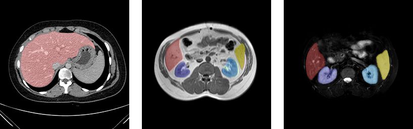
details of this dataset are given in Tab.2 and a sample case is All 2D slices were labeled manually by three different ra-
illustrated in Fig.3. diology experts who have 10, 12, and 28 years of experience,
respectively. The final shapes of the reference segmentations
were decided by majority voting. Also, in some extraordinary
3.2. Aims and Tasks
situations such as when inferior vena cava (IVC) is accepted
CHAOS challenge has two separate but related aims: as a part of the liver, experts have made joint decisions. In
CHAOS, voxels belong to IVC were excluded unless they are
1. achieving accurate segmentation of the liver from CT not completely inside of the liver. Although this handcrafted an-
scans, notation process has taken a significant amount of time, it was
preferred to create a consistent and consensus-based ground
2. reaching accurate segmentation of abdominal organs truth image series.
(liver, spleen, kidneys) from MRI sequences.
2 CHAOS description: https://chaos.grand-challenge.org/
1 CHAOS data information: https://chaos.grand-challenge.org/Data/ 3 CHAOS FAQ: https://chaos.grand-challenge.org/News and FAQ/5
Fig. 1. Example slices from CHAOS CT, MR (T1-DUAL in-phase) and MR (T2-SPIR) datasets (liver:red, right kidney:dark blue, left kidney:light blue
and spleen:yellow).
Fig. 2. 3D visualization of the liver from the CHAOS CT dataset (case 35). Fig. 3. 3D visualization of liver (red), right kidney (dark blue), left kidney
(light blue) and spleen (yellow) from the CHAOS MR dataset (case 40).
Table 2. Statistics about CHAOS CT and MRI datasets.
Specification CT MR
Number of patients (Train + Test) 20 + 20 20 + 20
Number of sets (Train + Test) 20 + 20 60 + 60*
In-plane spatial resolution 512 x 512 256 x 256
Number of axial slices in each examination [min-max] [78 - 294] [26 - 50]
Average axial slice number 160 32x3*
Total axial slice number 6407 3868x3*
X spacing (mm/voxel) left-right [min-max] [0.54 - 0.79] [0.72 - 2.03]
Y spacing (mm/voxel) anterior-posterior [min-max] [0.54 - 0.79] [0.72 - 2.03]
Slice thickness (mm) [min-max] [2.0 - 3.2] [4.4 - 8.0]
* MRI sets are collected from 3 different pulse sequences. For each patient, T1-DUAL registered in and oppose phases and
T2-SPIR MRI data are acquired.6
3.4. Challenge Setup and Distribution of the Data 4. Maximum symmetric surface distance (MSSD) metric is
the maximum Hausdorff distance between border voxels
Both CT and MRI datasets were divided into 20 sets for train- in S and G. The unit of this metric is millimeters (the
ing and 20 sets for testing. When dividing the sets into train- smaller, the better).
ing and testing, attention was paid to the fact that the cases in
both sets contain similar features (resolution, slice thickness, 4.2. Scoring System
age of patients) as stratification criteria. Typically, training data
In the literature, there are two main ways of ranking results
is presented with ground truth labels, while testing data only
via multiple metrics. One way is ordering the results by met-
contains original images. To provide sufficient data that con-
rics’ statistical significance with respect to all results. Another
tains enough variability, the datasets in the training data were
way is converting the metric outputs to the same scale and aver-
selected to represent all the difficulties that are observed on
aging all (Langville and Meyer, 2013). In CHAOS, we adopted
the whole database, such as varying Hounsfield range and non-
the second approach. Values coming from each metric have
homogeneous parenchyma texture of liver due to the injection
been transformed to span the interval [0, 100] so that higher val-
of contrast media in CT images, sudden changes in planar view
ues correspond to better segmentation. For this transformation,
and effect of bias field in MR images.
it was reasonable to apply thresholds in order to cut off unac-
The images are distributed as DICOM files to present the
ceptable results and increase the sensitivity of the correspond-
data in its original form. The only modification was remov-
ing metric. We are aware of the fact that decisions on metrics
ing patient-related information for anonymization. The ground
and thresholds have a very critical impact on ranking (Maier-
truths are also presented as image series to match the original
Hein et al., 2018). Instead of setting arbitrary thresholds, we
format. CHAOS data can be accessed with its DOI number via
used intra- and inter-user similarities among the experts who
zenodo.org webpage under CC-BY-SA 4.0 license (Kavur et al.,
created the ground truth. We asked them to repeat the annota-
2019). One of the important aims of the challenges is to pro-
tion process of the same patient sets several times. These col-
vide data for long-term academic studies. We expect that this
lections of reference masks were used for the calculation of our
data will be used not only for the CHAOS challenge but also for
metrics in a pair-wise manner. These values were used to spec-
other scientific studies such as cross-modality works or medical
ify the thresholds as given in Tab. 3. By using these thresholds,
image synthesis from different modalities.
two manual segmentations performed by the same expert on the
same CT data set resulted in liver volumes of 1491 mL and 1496
4. Evaluation mL. The volumetric overlap is found to be 97.21%, while RVD
is 0.347%, ASSD is 0.611 (0.263 mm), RMSD is 1.04 (0.449
mm), and MSSD is 13.038 (5.632 mm). These measurements
4.1. Metrics
yielded a total grade of 95.14. A similar analysis of the seg-
Since the outcomes of medical image segmentation are used mentation of the liver from MRI showed a slightly lower grade
for various clinical procedures, using a single metric for 3D of 93.01%.
segmentation evaluation is not a proper approach to ensure ac-
ceptable results for all requirements (Maier-Hein et al., 2018; Table 3. Summary of metrics and threshold values. ∆ represents longest
Yeghiazaryan and Voiculescu, 2015). Thus, in the CHAOS possible distance in the 3D image.
challenge, four different metrics are combined. The metrics
Metric name Best value Worst value Threshold
have been chosen among the most preferred ones in previ-
ous challenges (Maier-Hein et al., 2018) and to analyze results DICE 1 0 DICE >0.8
in terms of overlapping, volumetric, and spatial differences.
RAVD 0% 100% RAVD7
5. Participating Methods assigning the number of groups to 4. Data augmentation is ap-
plied by performing random mirroring of the first two axes of
In this section, we present the majority of the results from the cropped regions which is followed by random 90 degrees
the conference participants and the best two of the most signif- rotation along the last axis and intensity shift with contrast aug-
icant post-conference results collected among the online sub- mentations.
missions. To be specific, Metu MMLab and nnU-Net results IITKGP-KLIV: In order to accomplish multi-modality
belong to online submissions while others are from the con- segmentation using a single framework, a multi-task adversar-
ference session. Each method is assigned a unique color code ial learning strategy is employed to train a base segmentation
as shown in the figures and tables. The majority of the ap- network SUMNet (Nandamuri et al., 2019) with batch normal-
plied methods (i.e. all except IITKGP-KLIV) used variations ization. To perform adversarial learning, two auxiliary classi-
of U-Net, which is a Convolutional Neural Networks (CNN) fiers, namely C1 and C2, and a discriminator network, i.e. D,
approach that was first proposed by Ronneberger et al. (2015) are used. C1 is trained by the input from the encoder part of
for segmentation on biomedical images. This seems to be a typ- SUMNet which provides modality-specific features. C2 classi-
ical situation as the corresponding architecture dominates most fier is used to predict the class labels for the selected segmen-
of the recent DL based studies even in the presence of limited tation maps. The segmentation network and classifier C2 are
annotated data which is a typical scenario for biomedical im- trained using cross-entropy loss while the discriminator D and
age applications. Among all, two of them rely on ensembles auxiliary classifier C1 are trained by binary cross-entropy loss.
(i.e. MedianCHAOS and nnU-Net), which uses multiple mod- Adam optimizer is used for optimization. The input data to the
els and combine their results. network is the combination of all four modalities, i.e. CT, MRI
In the following paragraphs, the explanations of the partici- T1-DUAL in and oppose phases as well as MRI T2-SPIR.
pants’ methods are summarized. Also, brief comparisons of the
methods in terms of methodological details and training strat- METU MMLAB: This model is also designed as a varia-
egy, and pre-, post-processing and data augmentation strategies tion of U-Net. In addition, a Conditional Adversarial Network
are provided in Table 4 and Table 5, respectively. (CAN) is introduced in the proposed model. Batch Normaliza-
OvGUMEMoRIAL: A modified version of Attention U- tion is performed before convolution. In this way, vanishing
Net proposed in (Abraham and Khan, 2019) is used. Differently gradients are prevented and selectivity is increased. Moreover,
from the original UNet architecture (Ronneberger et al., 2015), parametric ReLU is employed to preserve the negative values
an Attention U-Net in (Abraham and Khan, 2019) soft attention using a trainable leakage parameter. In order to improve the per-
gates are used, multiscaled input image pyramid is employed formance around the edges, a CAN is employed during train-
for better feature representation, and Tversky loss is computed ing (not as a post-process operation). This introduces a new
for the four different scaled levels. The modification adopted loss function to the system which regularizes the parameters
by the OvGUMEMoRIAL team is that they employed paramet- for sharper edge responses. The only normalization of each CT
ric ReLU activation function instead of ReLU, where an extra image is performed for pre-processing and 3D connected com-
parameter, i.e. coefficient of leakage, is learned during train- ponent analysis is utilized for post-processing.
ing. Adam optimizer is used, training is accomplished by 120 PKDIA: The team proposed an approach based on con-
epochs with a batch size of 256. ditional generative adversarial networks where the generator is
ISDUE: The proposed architecture is constructed by three constructed by cascaded partially pre-trained encoder-decoder
main modules, namely 1) a convolutional autoencoder network networks (Conze et al., 2020b) extending the standard U-Net
which is composed of the prior encoder fenc p , and decoder gdec ; (Ronneberger et al., 2015) architecture. More specifically, first,
2) a segmentation hourglass network which is composed of the the standard U-Net encoder part is exchanged for a deeper net-
imitating encoder fenci , and decoder gdec ; 3) U-Net module, i.e. work, i.e. VGG-19 by omitting the top layers. Differently from
hunet , which is used to enhance the decoder gdec by guiding the the standard U-Net (Ronneberger et al., 2015), 1) 64 channels
decoding process for better localization capabilities. The seg- (32 channels for standard U-Net) are generated by the first con-
mentation networks, i.e. U-Net module and hourglass network volutional layer; 2) after each max-pooling operation, the num-
module, are optimized separately using the DICE loss and reg- ber of channels doubles until it reaches 512 (256 for standard U-
ularized by L sc with a regularization weight of 0.001. The au- Net); 3) second max-pooling operation is followed by 4 consec-
toencoder is optimized separately using DICE loss. Adam opti- utive convolutional layers instead of 2. For training, an Adam
mizer is used with initial learning rate of 0.001, batch size of 1 optimizer with a learning rate of 10−5 is used. Fuzzy DICE
is used and 2400 iterations are performed to train each model. score is employed as the loss function.
Data augmentation in performed by applying random transla- MedianCHAOS: Averaged ensemble of
tion and rotation operations during training. five different networks is used. The first one is the DualTail-
Lachinov: The proposed model is based on the 3D U-Net Net architecture that is composed of an encoder, central block
architecture, with skip connections between contracting and ex- and 2 dependent decoders. While performing downsampling by
panding paths and exponentially growing number of channels max-pooling operation, the max-pooling indices are saved for
across consecutive spatial resolution levels. The encoding path each feature map to be used during the upsampling operation.
is constructed by a residual network which provides efficient The decoder is composed of two branches: one that consists of
training. Group normalization (Wu and He, 2018) is adopted four blocks and starts from the central block of the U-net ar-
instead of batch normalization (Ioffe and Szegedy, 2015), by chitecture, and another one that consists of 3 blocks and starts8
from the last encoder block. These two branches are processed nnU-Net: The nnU-Net team participated in the challenge
in parallel where the corresponding feature maps are concate- with an internal variant of nnU-Net (Isensee et al., 2019), which
nated after each upsampling operation. The decoder is followed is the winner of Medical Segmentation Decathlon (MSD) in
by a 1 × 1 convolution and sigmoid activation function which 2018, (Simpson et al., 2019). They have made submissions for
provides a binary segmentation map at the output. Task 3 and Task 5. These tasks need to process T1-DUAL in
Other four networks are U-Net architecture variants, i.e. Ter- and oppose phase images as well as T2-SPIR images. While
nausNet (U-Net with VGG11 backbone (Iglovikov and Shvets, the T1-DUAL images are registered and can be used a separate
2018)), LinkNet34 (Shvets et al., 2018), and two networks color channel inputs, it was not chosen to do so because this
with ResNet-50 and SE-Resnet50. The latter two were both would have required substantial modification to nnU-Net (2 in-
pretrained on ImageNet encoders and decoders and consist of put modalities for T1-DUAL, 1 input modality for T2-SPIR).
convolution, ReLU and transposed convolutions with stride 2. Instead, T1-DUAL in and out phases were treated as separate
The two best final submissions were the averaged ensembles training examples, resulting in a total of 60 training examples
of predictions obtained by these five networks. The training for the aforementioned tasks.
process for each network was performed with Adam optimizer. No external data was used. Task 3 is a subset of Task 5, so
DualTail-Net and LinkNet34 were trained with soft DICE loss training was done only once and the predictions for Task 3 were
and the other three networks were trained with the combined generated by isolating the liver label. The submitted predictions
loss: 0.5*soft DICE + 0.5*BCE (binary cross-entropy). No ad- are a result of an ensemble of three 3D U-Nets (“3d fullres”
ditional post-processing was performed. configuration of nnU-Net). The five models originate from
Mountain: A 3D network architecture modified from the cross-validation on the training cases. Furthermore, since only
U-Net in (Han et al., 2019) is used. Differently from U-Net in one prediction is accepted for both T1-DUAL image types, an
(Ronneberger et al., 2015), in (Han et al., 2019) a pre-activation ensemble of the predictions of T1-DUAL in and oppose phases
residual block in each scale level is used at the encoder part; were used.
instead of max pooling, convolutions with stride 2 to reduce the
spatial size is employed; and instead of batch normalization, 6. Results
instance normalization (Ulyanov et al., 2017) is used since in-
stance normalization is invariant to linear changes of intensity The training dataset was published approximately three
of each individual image. Finally, it sums up the outputs of all months before the ISBI 2019. The testing dataset was given 24
levels in the decoder as the final output to encourage conver- hours before the challenge session. The submissions were eval-
gence. Two networks adopting the aforementioned architecture uated during the conference, and the winners were announced.
with different number of channels and levels are used here. The After ISBI 2019, training and testing datasets were published
first network, NET1, is used to locate an organ such as the liver. on zenodo.org website (Kavur et al., 2019) and the online sub-
It outputs a mask of the organ to crop out the region of interest mission system was activated on the challenge website.
to reduce the spatial size of the input to the second network, To compare the automatic DL methods with semi-automatic
NET2. The output of NET2 is used as the final segmentation ones, interactive methods including both traditional iterative
of this organ. Adam optimizer is used with the initial learning models and more recent techniques are employed from our pre-
rate = 1 × 10⁻³ , β1 = 0.9, β2 = 0.999, and = 1 × 10⁻⁸ . DICE vious work (Kavur et al., 2020). In this respect, we report the
coefficient was used as the loss function. Batch size was set to results and discuss the accuracy and repeatability of emerging
1. Random rotation, scaling, and elastic deformation were used automatic DL algorithms with those of well-established interac-
for data augmentation during training. tive methods, which are applied by a team of imaging scientists
CIR MPerkonigg: In order to train the network jointly for and radiologists through two dedicated viewers: Slicer (Kikinis
all modalities, the IVD-Net architecture of (Dolz et al., 2018) is et al., 2014) and exploreDICOM (Fischer et al., 2010).
employed. It follows the structure of U-Net (Ronneberger et al., There exist two separate leaderboards at the challenge web-
2015) with a number of modifications listed as follows: site, one for the conference session4 and another for post-
conference online submissions5 . Detailed metric values and
1) Dense connections between encoder path of IVD-Net are
converted scores are presented in Tab.8. Box plots of all results
not used since no improvement is obtained with that scheme,
for each task are presented separately in Fig.7. Also, scores on
2) During training, images from all modalities are not fed each testing case are shown in Fig.8 for all tasks. As expected,
into the network at all times. the tasks, which received the highest number of submissions
Residual convolutional blocks (He et al., 2016) are used. and scores, were the ones focusing on the segmentation of a sin-
Data augmentation is performed by accomplishing affine trans- gle organ, from a single modality. Thus, the vast majority of the
formations, elastic transformations in 2D, histogram shifting, submissions were for liver segmentation from CT images (Task
flipping and Gaussian noise addition. In addition, Modality 2), followed by liver segmentation from MR images (Task 3).
Dropout (Li et al., 2016) is used as the regularization technique Accordingly, in the following subsections, the results are pre-
where modalities are dropped with a certain probability when sented in the order of performance/participation in Tab.6 (i.e.
the training is performed using multiple modalities which helps
decrease overfitting on certain modalities. Training is done
by using Adam optimizer with a learning rate of 0.001 for 75 4 https://chaos.grand-challenge.org/Results CHAOS/
epochs. 5 https://chaos.grand-challenge.org/evaluation/results/9
Table 4. Brief comparison of participating methods
Team Details of the method Training strategy
OvGUMEMoRIAL •Modified Attention U-Net (Abraham and Khan, 2019), employing soft attention •Tversky loss is computed for the four different scaled levels.
(P. Ernst, S. Chatterjee, O. Speck, gates and multiscaled input image pyramid for better feature representation is used.
A. Nürnberger)
•Adam optimizer is used, training is accomplished by 120 epochs
•Parametric ReLU activation is used instead of ReLU, where an extra parameter, with a batch size of 256.
i.e. coefficient of leakage, is learned during training.
ISDUE •The proposed architecture consists of three main modules: •The segmentation networks are optimized separately using the
(D. D. Pham, G. Dovletov, DICE-loss and regularized by L sc with weight of λ = 0.001.
J. Pauli)
i. Autoencoder net composed of a prior encoder fenc p , and decoder gdec ;
ii. Hourglass net composed of an imitating encoder fenci , and decoder gdec ; •The autoencoder is optimized separately using DICE loss.
iii. U-Net module, i.e. hunet , which is used to enhance the decoder gdec by guiding
the decoding process for better localization capabilities. •Adam optimizer with an initial learning rate of 0.001, and 2400
iterations are performed to train each model.
Lachinov •3D U-Net, with skip connections between contracting/expanding paths and •The network was trained with ADAM optimizer with learn-
(D. Lachinov) exponentially growing number of channels across consecutive resolution levels ing rate 0.001 and decaying with a rate of 0.1 at 7th and 9th epoch.
(Lachinov, 2019).
•The network is trained with batch size 6 for 10 epochs. Each
•The encoding path is constructed by a residual network for efficient training. epoch has 3200 iterations in it.
•Group normalization (Wu and He, 2018) is adopted instead of batch (Ioffe and
Szegedy, 2015) (# of groups = 4). •The loss function employed is DICE loss.
•Pixel shuffle is used as an upsampling operator
IITKGP-KLIV •To achieve multi-modality segmentation using a single framework, a multi-task •The segmentation network and C2 are trained using cross-
(R. Sathish, R. Rajan, D. Sheet) adversarial learning strategy is employed to train a base segmentation network entropy loss while the discriminator D and auxiliary classifier C1
SUMNet (Nandamuri et al., 2019) with batch normalization. are trained by binary cross-entropy loss.
•Adversarial learning is performed by two auxiliary classifiers, namely C1 and C2, •Adam optimizer. Input is the combination of all four modalities,
and a discriminator network D. i.e. CT, MRI T1 DUAL In and Oppose Phases, MRI T2 SPIR.
METU MMLAB •A U-Net variation and a Conditional Adversarial Network (CAN) is introduced. •To improve the performance around the edges, a CAN is
(S. Özkan, B. Baydar, G. B. Akar) employed during training (not as a post-process operation).
•Batch Normalization is performed before convolution to prevent vanishing
gradients and increase selectivity. •This introduces a new loss function to the system which regular-
izes the parameters for sharper edge responses.
•Parametric ReLU to preserve negative values using a trainable leakage parameter.
PKDIA (P.-H. Conze) •An approach based on Conditional Generative Adversarial Networks (cGANs) is •An Adam optimizer with a learning rate of 10−5 is used.
proposed: the generator is built by cascaded pre-trained encoder-decoder (ED) net-
works (Conze et al., 2020b) extending the standard U-Net (sU-Net) (Ronneberger •Fuzzy DICE score is employed as loss function.
et al., 2015) (VGG19, following (Conze et al., 2020a)), with 64 channels (instead
of 32 for sU-Net) generated by first convolutional layer. •Batch size was set to 3 for CT and 5 for MR scans.
•After each max-pooling, channel number doubles until 512 (256 for sU-Net). Max-
pooling followed by 4 consecutive conv. layers instead of 2. The auto-context
paradigm is adopted by cascading two EDs (Yan et al., 2019): the output of the
first is used as features for the second.
•Averaged ensemble of five different networks is used. The first one is DualTail-Net •The training for each network was performed with Adam.
MedianCHAOS that is composed of an encoder, central block and 2 dependent decoders.
(V. Groza)
•DualTail-Net and LinkNet34 were trained with soft DICE loss
•Other four networks are U-Net variants, i.e. TernausNet (U-Net with VGG11 back- and the other three networks were trained with the combined loss:
bone (Iglovikov and Shvets, 2018)), LinkNet34 (Shvets et al., 2018), and two with 0.5*soft DICE + 0.5*BCE (binary cross-entropy).
ResNet-50 and SE-Resnet50.
Mountain (Shuo Han) •3D network adopting U-Net variant in (Han et al., 2019) is used. It differs from •Adam optimizer is used with the initial learning rate = 1 × 10⁻³ ,
U-Net in (Ronneberger et al., 2015), by adopting: i. A pre-activation residual block β1 = 0.9, β2 = 0.999, and = 1 × 10⁻⁸ .
in each scale level at the encoder, ii. Convolutions with stride 2 to reduce the spatial
size, iii. Instance normalization (Ulyanov et al., 2017). •DICE coefficient was used as the loss function. Batch size was
set to 1.
•Two nets, i.e. NET1 and NET2, adopting (Han et al., 2019) with different channels
and levels. NET1 locates organ and outputs a mask for NET2 performing finer
segmentation.
CIRMPerkonigg •For joint training with all modalities, the IVD-Net (Dolz et al., 2018) (which •Modality Dropout (Li et al., 2016) is used as the regularization
(M. Perkonigg) is an extension of U-Net Ronneberger et al. (2015)) is used with a number of technique to decrease over-fitting on certain modalities.
modifications:
i. dense connections between encoder path of IVD-Net are not used since no •Training is done by using Adam optimizer with a learning rate
improvement is achieved of 0.001 for 75 epochs.
ii. training images are split.
•Moreover, residual convolutional blocks (He et al., 2016) are used.
nnU-Net •An internal variant of nnU-Net (Isensee et al., 2019), which is the winner of •T1 in and out are treated as separate training examples, resulting
(F. Isensee, K. H. Maier-Hein) Medical Segmentation Decathlon (MSD) in 2018 (Simpson et al., 2019), is used. in a total of 60 training examples for the tasks.
•Ensemble of five 3D U-Nets (“3d fullres” configuration), which originate from •Task 3 is a subset of Task 5, so training was done only once and
cross-validation on the training cases. Ensemble of T1 in and oppose phases was the predictions for Task 3 were generated by isolating the liver.
used.10
Table 5. Pre-, post-processing, data augmentation operations and participated tasks.
Team Pre-process Data augmentation Postprocess Tasks
OvGUMEMoRIAL Training with resized images - Threshold by 0.5 1,2,3,4,5
(128 × 128). Inference: full-sized.
ISDUE Training with resized images Random translate and rotate Threshold by 0.5. Bicubic 1,2,3,4,5
(96,128,128) interpolation for refinement.
Lachinov Resampling 1.4 × 1.4 × 2 z-score Random ROI crop 192 × 192 × 64, Threshold by 0.5 1,2,3
normalization mirror X-Y, transpose X-Y, Window
Level - Window Width
IITKGP-KLIV Training with resized images - Threshold by 0.5 1,2,3,4,5
(256 × 256), whitening. Additional
class for body.
METUMMLAB Min-max normalization for CT - Threshold by 0.5. Connected 1,3,5
component analysis for
selecting/eliminating some of the
model outputs.
PKDIA Training with resized Random scale, rotate, shear and shift Threshold by 0.5. Connected 1,2,3,4,5
images: 256 × 256 MR, 512 × 512 component analysis for
CT. selecting/eliminating some of the
model outputs.
LUT [-240,160] HU range, - Threshold by 0.5. 2
MedianCHAOS normalization.
Mountain Resampling 1.2 × 1.2 × 4.8, zero Random rotate, scale, elastic Threshold by 0.5. Connected 3,5
padding. Training with resized deformation component analysis for
images: 384 × 384 × 64. Rigid selecting/eliminating some of the
register MR. model outputs.
CIRMPerkonigg Normalization to zero mean unit 2D Affine and elastic transforms, Threshold by 0.5. 3
variance. histogram shift, flip and adding
Gaussian noise.
nnU-Net Normalization to zero mean unit Add Gaussian noise / blur, rotate, Threshold by 0.5. 3,5
variance, Resampling 1.6 × 1.6 × 5.5 scale, WL-WW, simulated low
resolution, Gamma, mirroring
Table 6. CHAOS challenge submission statistics for on-site and online sessions.
Submission numbers Task 1 Task 2 Task 3 Task 4 Task 5 Total
ISBI 2019 5 14 7 4 5 35
Online 20 263 42 15 71 -
The most by the same team (ISBI 2019) 0 5 0 0 0 -
The most by the same team (Online) 3 8 8 2 7 -
from the task having the highest submissions to the one hav- Peeking makes it possible to use testing data for validation pur-
ing the lowest). In this way, the segmentation from cross- and poses (i.e., for parameter tuning) even without accessing its
multi-modality/organ concepts (Tasks 1 and 4) are discussed in ground truths and pointed as one of the shortcomings of the
the light of the performances obtained for more conventional image segmentation grand-challenges.
approaches (Tasks 2, 3 and 5).
Comparison of a fair development and peeking attempts is
shown in Fig.4. Peeking is surprisingly an under-estimated
6.1. Remarks about Multiple Submissions
problem in academic studies, which causes over-fitting of al-
Although testing datasets should only be considered as the gorithms (especially deep models) on target data. Therefore,
unseen (new) data provided to the algorithms, there is a way successful models tuned for a specific dataset may not be use-
to use them for algorithm development stage. This way is ful for real-world problems resulting in a loss of generalization
called “peeking” which is done through reporting too many per- ability. The effect of peeking on the score of some participat-
formance results by iterative submissions (Kuncheva (2014)). ing teams from CHAOS online leaderboard are given in Tab.7.11
Development stage Evaluation stage
Training on
train data
Evaluation
Algorithm Final Score
Developing (on test data)
Validation on
Parameter
validation
tuning
data
Development stage Peeking cycle + Evaluation stage
Training on Submission
train data
Algorithm
Developing Final Score
Validation on Additional
Parameter Evaluation
validation parameter
tuning (on test data)
data tuning
Fig. 4. Illustration of a fair study (green area) and peeking attempts (red area)
a good opportunity to test the effectiveness of the participating
Table 7. Example results of possible peeking attempts that have been ob-
tained from online results of CHAOS challenge. The impact of peeking can models compared to the existing approaches. Although the pro-
be observed from score changes. (Team names were anonymized.) vided datasets only include healthy organs, the injection of con-
trast media creates several additional challenges, as described in
Number of iterative
Participant Score change Section III.B. Nevertheless, the highest scores of the challenge
submissions
were obtained in this task (Fig.7b).
Team A 21 +29.09% The on-site winner was MedianCHAOS with a score of
Team B 19 +15.71% 80.45±8.61 and the online winner is PKDIA with 82.46±8.47.
Being an ensemble strategy, the performances of the sub-
Team C 16 +12.47%
networks of MedianCHAOS are illustrated in Fig. 8.c. When
Team D 15 +30.02% individual metrics are analyzed, DICE performances seem to
Team E 15 +26.06% be outstanding (i.e. 0.98±0.00) for both winners (i.e. scores
97.79±0.43 for PKDIA and 97.55±0.42 for MedianCHAOS).
Team F 13 +10.10%
Similarly, ASSD performances have very high mean and small
variance (i.e. 0.89±0.36 [score: 94.06±2.37] for PKDIA and
0.90±0.24 [94.02±1.6] for MedianCHAOS). On the other hand,
These results show that, the impact of the peeking can be note-
RAVD and MSSD scores are significantly low resulting in re-
worthy in some cases. For this reason, in this paper, we have
duced overall performance. Actually, this outcome is valid for
included only the studies (mostly from on-site submissions) in
all tasks and participating methods.
which we could verify their results are consistent and reliable.
There is single score announcement at the end of the on-site Regarding semi-automatic approaches in (Kavur et al.,
challenge session that makes peeking impossible. On the other 2020), the best three have received scores 72.8 (active contours
hand, the online participated methods presented in this article with a mean interaction time (MIT) of 25 minutes ), 68.1 (ro-
have shown their success in multiple challenges and their source bust static segmenter having a MIT of 17 minutes), and 62.3
codes are shared in open platforms. Therefore, the fairness of (i.e. watershed with MIT of 8 minutes). Thus, the successful
these studies could be confirmed. designs among participants in deep learning-based automatic
segmentation algorithms have outperformed the interactive ap-
6.2. CT Liver Segmentation (Task 2) proaches by a large margin. This increase reaches almost to
This task includes one of the most studied cases and a very the inter-expert level for volumetric analysis and average sur-
mature field of abdominal segmentation. Therefore, it provides face differences. However, there is still a need for improvement12
MedianCHAOS6
IITKGP-KLIV
OvGUMEMoRIAL
ISDUE
PKDIA
Lachinov
MedianCHAOS3
MedianCHAOS5 MedianCHAOS2
MedianCHAOS4
MedianCHAOS1
Fig. 5. Example image from the CHAOS CT dataset, (case 35, slice 95), borders of segmentation results on ground truth mask (cropped to liver), and
zoomed onto inferior vena cava (IVC) region (marked with dashed lines on the middle image) respectively. Since the contrast between liver tissue and IVC
is relatively lower due to timing error during CT scan, algorithms make the most mistakes here. On the other hand, many of them are quite successful in
other regions of the liver.
considering the metrics related to maximum error margins (i.e. [score: 89.58±4.54] for PKDIA) performances are again ex-
RAVD and MSSD). An important drawback of the deep ap- tremely good, while RAVD and MSSD scores are significantly
proaches is observed as they might completely fail and generate lower than the CT results. The reason behind this can also be
unreasonably low scores for particular cases, such as the infe- attributed to lower resolution and higher spacing of the MR
rior vena cava region shown in Fig.5. data, which cause a higher spatial error for each mis-classified
Regarding the effect of architectural design differences pixel/voxel (see Tab.2). Comparisons with the interactive meth-
on performance, comparative analyses have been per- ods show that they tend to make regional mistakes due to the
formed through some well established deep frameworks (i.e. spatial enlargement strategies. The main challenge for them
DeepMedic (Kamnitsas et al., 2017) and NiftyNet (Gibson is to differentiate the outline when the liver is adjacent to iso-
et al., 2018)). These models have been applied with their de- dense structures. On the other hand, automatic methods show
fault parameters and they have both achieved scores around 70. much more distributed mistakes all over the liver. Further anal-
Thus, considering the participating models that have received ysis also revealed that interactive methods seem to make fewer
below 70, it is safe to conclude that, even after the intense re- over-segmentations. This is partly related to iterative parameter
search studies and literature, the new deep architectural designs adjustment of the operator which prevents unexpected results.
and parameter tweaking does not necessarily translate into more Overall, the participating methods performed equally well with
successful systems. interactive methods if only volumetric metrics are considered.
However, the interaction seems to outperform deep models for
other metrics.
6.3. MR Liver Segmentation (Task 3)
Segmentation from MR can be considered as a more diffi- 6.4. CT-MR Liver (Cross-Modality) Segmentation (Task 1)
cult operation compared to segmentation from CT because CT This task targets cross-modality learning and it involves the
images have a typical histogram and dynamic range defined usage of CT and MR information together during training. A
by Hounsfield Units (HU), whereas MRI does not have such model that can effectively accomplish cross-modality learning
a standardization. Moreover, the artifacts and other factors in would: 1) help to satisfy the big data needs of deep models by
clinical routine cause significant degradation of the MR im- providing more images and 2) reveal common features of in-
age quality. The on-site winner of this task is PKDIA with a corporated modalities for an organ. To compare cross-modality
score of 70.71±6.40. PKDIA had the most successful results learning with individual ones, Fig.8a should be compared to
not only for the mean score but also for the distribution of the Fig.8c for CT. Such a comparison clearly reveals that partici-
results (shown in Fig.7c and 8d). Robustness to the deviations pating models trained only on CT data show significantly better
in MR data quality is an important factor that affects perfor- performance than models trained on both modalities. A simi-
mance. For instance, CIR MPerkonigg, which has the most lar observation can also be made for MR results by observing
successful scores for some cases, but could not show an high Fig.8b and Fig.8d.
overall score. The on-site winner of this task was OvGUMEMoRIAL with
The online winner is nnU-Net with 75.10±7.61. When the a score of 55.78±19.20. Although its DICE performance is
scores of individual metrics are analyzed for PKDIA and nnU- quite satisfactory (i.e. 0.88±0.15, corresponding to a score of
Net, DICE (i.e. 0.94±0.01 [score: 94.47±1.38] for PKDIA 83.14±0.43), the other measures cause the low grade. Here, a
and 0.95±0.01 [score: 95.42±1.32] for nnU-Net) and ASSD very interesting observation is that the score of OvGUMEMo-
(i.e. 1.32±0.83 [score: 91.19±5.55] for nnU-Net and 1.56±0.68 RIAL is lower than its score on CT (61.13±19.72) but higher13
than MR (41.15±21.61). Another interesting observation of the maps reveal better performance (DICE: 0.87 ± 0.05) compared
highest-scoring non-ensemble model, PKDIA, both for Task 2 to some other models such as U-net (Ronneberger et al., 2015)
(CT) and Task 1 (MR), had a significant performance drop in (DICE: 0.81 ± 0.08), DANet (Fu et al., 2019) (DICE: 0.83 ±
this task. Finally, it is worth to point that the online results have 0.10), PAN(ResNet) (Li et al., 2018) (DICE: 0.84 ± 0.06), and
reached up to 73, but those results could not be validated (i.e. UNet Attention (Schlemper et al., 2019) (DICE: 0.85 ± 0.05).
participant did not respond) and achieved after multiple submis- Despite these slight improvements caused by novel archi-
sions by the same team. In such cases, the possibility of peeking tectural designs, the performance of the proposed models still
is very strong and therefore, not included in the manuscript. seem to below the best three contestants (i.e. nnUnet-0.95 ±
It is important to examine the scores of cases with their distri- 0.02, PKDIA-0.93 ± 0.02 and Mountain- 0.90 ± 0.03) of the
bution across all data. This can help to analyze the generaliza- CHAOS challenge. This is also observed for other metrics such
tion capabilities and real-life use of these systems. For exam- as ASSD (OvGUMEMoRIAL: 1.05 ± 0.55). Nevertheless, the
ple, Fig.7.a shows a noteworthy situation. The winner of Task 1, modifications of (Sinha and Dolz, 2020) reduced the standard
OvGUMEMoRIAL, shows lower performances than the second deviation of the other metrics rather than their mean values.
method (ISDUE) in terms of standard deviation. Fig.8a and 8b The qualitative analysis performed to visualize the effect of pro-
show that the competing algorithms have slightly higher scores posed modifications illustrate that some models (such as UNet)
on the CT data than on the MR data. However, if we consider typically under-segments certain organs, produce smoother seg-
the scattering of the individual scores along with the data, CT mentations causing loss of fine grained details. The architec-
scores have higher variability. This shows that reaching equal tural modifications are especially helpful to compensate such
generalization for multiple modalities is a challenging task for drawbacks by focusing the attention of the model to anatomi-
Convolutional Neural Networks (CNNs). cally more relevant areas.
6.5. Multi-Modal MR Abdominal Organ Segmentation (Task 5)
6.6. CT-MR Abdominal Organ Segmentation (Cross-Modality
Task 5 investigates how DL models contribute to the develop- Multi Modal) (Task 4)
ment of more comprehensive computational anatomical models
leading to multi-organ related tasks. Deep models have the po- This task covers segmentation of both the liver in CT and
tential to provide a complete representation of the complex and four abdominal organs in MRI data. Hence, it can be considered
flexible abdominal anatomy by incorporating inter-organ rela- as the most difficult task since it contains both cross-modality
tions through their internal hierarchical feature extraction pro- learning and multiple organ segmentation. Therefore, it is not
cesses. surprising that it has the lowest attendance and scores.
The on-site winner was PKDIA with a score of 66.46±0.81 The on-site winner was ISDUE with a score of 58.69±18.65.
and the online winner is nnU-Net with 72.44±5.05. When the Fig. 8.e-f shows that their solution had consistent and high-
scores of individual metrics are analyzed in comparison to Task performance distribution in both CT and MR data. It can be
3, the DICE performances seems to remain almost the same thought that two convolutional encoders in their system boost
for nnU-Net and PKDIA. This is a significant outcome as all performance on cross-modality data. These encoders are able
four organs are segmented instead of a single one. It is also to compress information about anatomy. On the other hand,
worth to point that the model of the third-place (i.e. Moun- PKDIA also shows promising performance with a score of
tain) has almost exactly the same overall score for Task 3 and 49.63±23.25. Despite their success on MRI sets, the CT per-
5. The same observation is also valid for the standard devi- formance can be considered unsatisfactory, similar to their sit-
ation of these models. Considering RAVD, the performance uation at Task 1. This reveals that the CNN-based encoder may
decrease seems to be higher compared to DICE. These reduced not efficiently be trained. The encoder part of their solution
DICE and RAVD performances are partially compensated by relies on transfer learning, fine tuning the pre-trained weights
better MSSD and ASSD performances. On the other hand, this were not successful on multiple modalities. The OvGUMEMo-
increase might not be directly related to multi-organ segmenta- RIAL team achieved the third position with an average score
tion. One should keep in mind that generally the most complex of 43.15 and they have a balanced performance on both modal-
abdominal organ for segmentation is the liver (Task 3) and the ities. Their method can be considered successful in terms of
other organs in Task 5 can be considered relatively easier to generalization, among the participating teams.
analyze. Together with the outcomes of Task 1 and 5, it is shown that
Follow up studies, which did not participate to the challenge, in current strategies and architectures, CNNs have better seg-
but used the CHAOS dataset, have also recently reported re- mentation performance on single modality tasks. This might
sults for this task. Considering an attention-based model (Wang be considered as an expected outcome because the success of
et al., 2018) as the baseline (DICE: 0.83 ± 0.06), an ablation CNNs is very dependent on the consistency and homogeneity
study is carried out to that increase the segmentation perfor- of the data. Using multiple modalities creates a high variance
mance (Sinha and Dolz, 2020). The limitations of the baseline in the data even though all data were normalized. On the other
is tried to be improved by capturing richer contextual dependen- hand, the results also revealed that CNNs have good potential
cies through guided self-attention mechanisms. Architectural for cross-modality tasks if appropriate models are constructed.
modifications for integrating local features with their global de- This potential was not that clear before the development of deep
pendencies and adaptive highlighting of interdependent channel learning strategies for segmentation.You can also read