Chase and Flight: New Product Diffusion with Social Attraction and Repulsion
←
→
Page content transcription
If your browser does not render page correctly, please read the page content below
Chase and Flight: New Product Diffusion with Social
             Attraction and Repulsion
                                                  Nitin Bakshi
                         London Business School, London, UK NW1 4SA, nbakshi@london.edu

                                               Kartik Hosanagar
       The Wharton School, University of Pennsylvania, Philadelphia, PA 19104-6340, kartikh@wharton.upenn.edu

                                          Christophe Van den Bulte
       The Wharton School, University of Pennsylvania, Philadelphia, PA 19104-6340, vdbulte@wharton.upenn.edu

   Asymmetric attraction and repulsion between consumer segments has quickly become a major topic among
   marketers and consumer researchers. For example, middle class consumers often emulate the adoption deci-
   sions of the elite whereas the latter prefer to use products that help distinguish them from the middle class.
   This can result in a chase-and-flight pattern where the elite starts disadopting once the product or practice
   has become too popular with the outsiders emulating it. We present a mathematical model of new product
   diffusion featuring asymmetric attraction and repulsion between customer segments and provide an analyti-
   cal and visual characterization of the chase-and-flight diffusion dynamics. We identify potential equilibrium
   outcomes and specify conditions under which the product can achieve full market potential in both market
   segments. We also identify which early diffusion trajectories are likely to lead to complete acceptance by
   both segments versus complete rejection by one segment. Finally, we provide insights into the effectiveness
   of several marketing policies to counter the repulsion effect. A number of accepted notions about optimal
   market seeding do not always apply in markets with joint attraction/repulsion.
   Subject Classifications: New products; customer segmentation
   Area of Review: Marketing

   Key words : social contagion; word-of-mouth; adoption of innovations; chase-and-flight; new product
     diffusion; marketing strategy; market seeding
   History : July 2, 2013

1. Introduction
People use products as both bridges and fences (Douglas and Isherwood 1979). Consumers imitate
the choices of those they are attracted to and would like to be identified with, but also choose
products and brands to distinguish themselves from those they do not want to be confused with.
These two forces can be at odds with each other. For instance, middle-class consumers often like to
emulate the choices of the elite, but the latter dislike this and prefer products that help distinguish
them from those below them (e.g., Bourdieu 1984; Simmel 1904). Such attraction/repulsion dynam-
ics create what McCracken (1988) called a “chase-and-flight” pattern: as one group chases another

                                                         1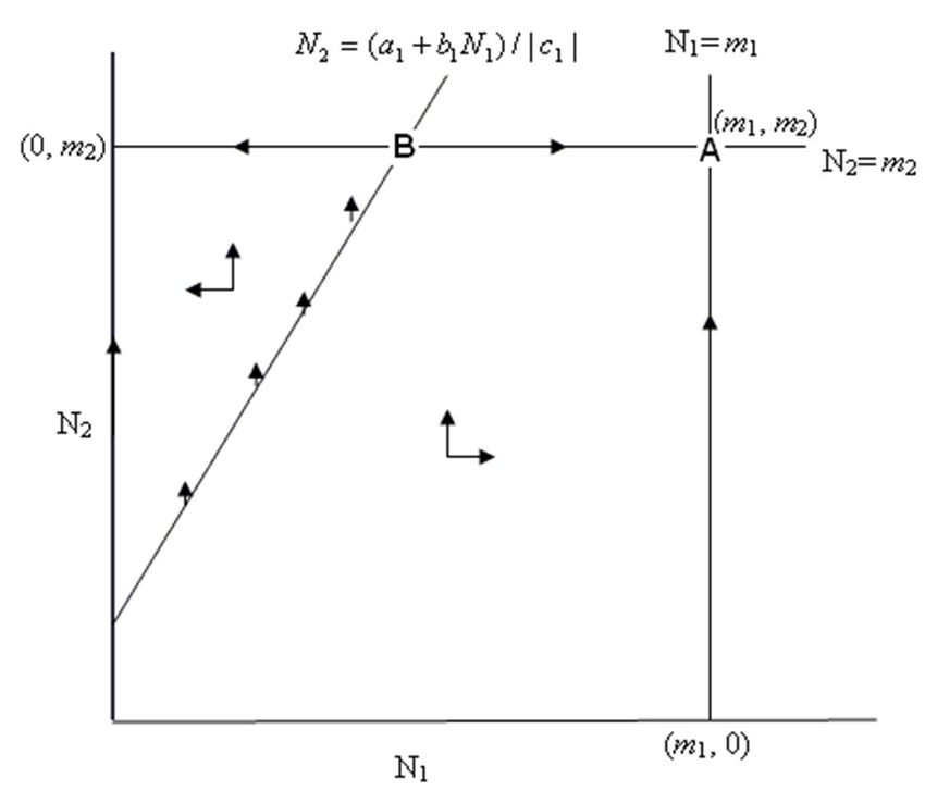
Bakshi, Hosanagar and Van den Bulte: Chase and Flight
2                                                       Article submitted to Operations Research; manuscript no.

group and flocks to products and practices popular with it, the second group starts deserting
these very same products and practices. So, attraction/repulsion and the resulting chase-and-flight
dynamic create a challenge for firms. They need their new products to be successful among the
elite to stimulate demand among other consumers, but success in the mass market will drive the
elite away from the product.
    Understanding and managing new product growth with asymmetric attraction/repulsion
between segments is especially important for status-oriented brands. Burberry, for instance, lost
both sales and stature among its traditional upper-class customer base when English hooligans
and other “riff-raff” started wearing the iconic plaid in the late 1990s (Moon 2004). Asymmetric
attraction/repulsion dynamics may also occur in more mundane product categories and within
rather than across economic strata, especially for products and brands associated with particu-
lar lifestyles or consumer identities. Black & Decker, for instance, saw professional craftsmen and
construction workers veer away from its power tools once they became “too popular” among the
casual do-it-yourself amateurs. Porsche, the famed maker of high-performance sports cars like the
iconic 911, faced a similar problem with the introduction of the Cayenne, its first sports utility
vehicle (SUV). Market research showed that well-heeled potential buyers of SUVs were favorably
disposed towards the Porsche brand, but having it become associated with soccer moms was bound
to displease the core segment of Porsche sports-car enthusiasts (Joshi et al. 2009). Diesel Jeans,
which nurtured a very “edgy” and “alternative” image appealing to contrarians, faced similar prob-
lems when it became successful among mainstream customers (Grigorian and Chandon 2004). The
risk and deleterious consequences of such “brand hijacking” by a particular segment are especially
pronounced for products with asymmetric attraction/repulsion between segments, regardless of
whether consumers are driven by “vertical” status or “horizontal” social identity considerations.
    These complex dynamics have long been discussed in sociology in general conceptual terms
(Bourdieu 1984; Simmel 1904). More recently, a wealth of laboratory evidence has appeared doc-
umenting how attraction and repulsion among customer groups affects customer preferences (e.g.,
Berger and Heath 2008; Berger and Le Mens 2009; Han et al. 2010; White and Dahl 2006). Formal
analytical work has focused on two-period settings (e.g., Amaldoss and Jain 2008), generated only
very vague results about possible diffusion trajectories (Miller et al. 1993), or has modeled the
process without allowing attractive customers to disadopt the product, hence curtailing the force
of repulsion (Joshi et al. 2009) and a central feature of the chase-and-flight phenomenon and theory
(Simmel 1904). Though the question of how attraction/repulsion between segments affects new
product acceptance is of great interest to both managers and researchers, current work offers only
limited analytic results about new product diffusion patterns in such market settings (Van den
Bulte et al. 2010).
Bakshi, Hosanagar and Van den Bulte: Chase and Flight
Article submitted to Operations Research; manuscript no. 3
Repulsion results in flight from potential adopters, but does it also lead prior adopters to flee
and disadopt? It very often does, the one exception being situations with very high switching costs.
Men may become less inclined to buy a Porsche Cayenne as the car becomes more popular among
women, but current owners—though disgruntled—may not be willing or able to simply ditch their
Cayenne car and buy a luxury SUV. So, for very expensive durable goods, repulsion need not
lead to disadoption and it is quite appropriate not to allow the first segment’s hazard rate to
turn negative (Joshi et al. 2009). Many products, services and practices, however, are either not
as expensive or durable, so repulsion can and does lead flight by prior adopters or disadoption.
The classic example is of course fashion apparel. Others include relatively inexpensive durables
that people can easily decide not to use anymore. Once earbuds become popular with mainstream
consumers, for instance, hipsters and hardcore fans of street music reverted back to old-school
over-the-ear headphones. “Cool” students have been observed to stop wearing bicycling helmets or
yellow Livestrong wristbands once they felt too may geeks had started doing so (Berger and Heath
2008). Of course, disadoption is also quite easy for services. Some pundits have voiced the concern
that, as Facebook becomes increasingly popular with adults and even elderly, teenagers will find
it attractive to migrate to other networking platforms like Twitter and Tumblr. Frequenting vs.
avoiding particular bars, fitness clubs, or restaurants is another social arena where we see the chase-
and-flight dynamic between famous, cool or other elite people and their wannabes. Yogi Berra once
explained why he no longer went to Ruggeri’s, a St. Louis restaurant, by noting: “Nobody goes
there anymore. It’s too crowded” (Berra meant, obviously, nobody who is anybody). So, a very
large class of products, services and practices, exhibit both chase and flight, both adoption and
disadoption.
We provide new insights about how a new product diffuses through such a market and about
some interventions a firm may undertake to increase its products success. To this end, we use the
following system of interlinked differential equations:
dN1
= (a1 + b1 N1 + c1 N2 )(m1 − N1 ); (1a)
dt
dN2
= (a2 + b2 N2 + c2 N1 )(m2 − N2 ), (1b)
dt
where the subscript i refers to one of two segments, and ai > 0, bi > 0, mi > 0, 0 ≤ Ni ≤ mi . Each
equation represents the change in user base of a new product in each of two segments (Table 1).
The c parameters capture the cross-segment influence. When c1 = c2 = 0, the model reduces to
two independent Bass (1969) model equations. When c1 = 0, c2 > 0, the model reduces to the
Asymmetric Influence Model studied by Van den Bulte and Joshi (2007). That model provides
valuable insights into new product diffusion with distinct segments of leaders and followers, butBakshi, Hosanagar and Van den Bulte: Chase and Flight
4 Article submitted to Operations Research; manuscript no.
cannot capture the attraction/repulsion effects which have gained much attention among both
practitioners and consumer researchers since their work appeared. When c1 < 0, c2 > 0, the model
represents new product growth with asymmetric attraction/repulsion between segments. Though
this model is inspired by Simmel (1904), c1 and c2 map into Veblen’s (1899) distinction between
“invidious comparison” (attempts by the high class to distinguish themselves from the lower class)
and “pecuniary emulation” (attempts by the lower class to be perceived as members of the high
class).
Table 1 Glossary of Terms
Ni number of users in segment i at time t (shorthand for Ni (t))
mi market potential for segment i
ai coefficient of innovation for segment i
bi coefficient of imitation or contagion within segment i
ci coefficient of imitation or contagion from segment j to segment i
When estimating this model to the Porsche Cayenne sales, Joshi et al. (2009) found the values
of both c1 and c2 to be significant, with the backlash or repulsion effect c1 being nearly six times
stronger than the attraction effect c2 . In addition to allowing c1 to be negative, a key feature of our
analysis is that we allow the first segments hazard rate (a1 + b1 N1 + c1 N2 ) to be negative, i.e., in
accordance with Simmel’s (1904) theory of fashion of chase-and-flight, we allow the repulsion effect
to be so large that it leads members of the imitated segment to actually disadopt the product rather
than to merely refrain from further adopting it. In recent experiments, Berger and Heath (2008)
show that repulsion can indeed lead to disadoption. In one of their studies, “cool” people stopped
wearing a wristband when “geeks” started wearing them. The authors concluded that “people may
abandon tastes adopted by other social groups to avoid signaling their characteristics”. So, allowing
flight or disadoption is important for providing a more truthful mathematical representation of
sociological and behavioral theory. As we demonstrate later in this paper, accounting for the
complete process of chase and flight also impacts the equilibrium outcomes.1
Even though the system described by (1a) and (1b) does not have a closed form solution, we still
obtain important insights about a new product’s success in markets with attraction and repulsion
between segments. First, we identify possible equilibrium outcomes. Specifically, we identify under
what circumstances the “elite” or “cool” segment stays with the product rather than dropping it
once the product becomes popular with the “wannabe” segment. Simmel’s influential theory of
fashion is predicated on this dynamic, but does it always have to happen? Also, what levels of
penetration can one obtain in each segment? Is it possible to end up in a situation where no one
in the imitated segment uses the product yet all people in the wannabe segment do? We find thatBakshi, Hosanagar and Van den Bulte: Chase and Flight
Article submitted to Operations Research; manuscript no. 5
irrespective of the strength of attraction and repulsion, the stable equilibrium outcomes belong
to the set {(0, m2 ), (m1 , m2 )}, where m1 and m2 are the market potential for segments 1 (“elite”)
and 2 (“wannabe”) respectively. Notably, equilibrium outcomes with intermediate values of market
penetration do arise, but these are always unstable.
Second, we identify which early diffusion trajectories are likely to lead to complete acceptance
by both segments versus complete rejection by one segment. Phase-plane analysis enables one to
clearly demarcate regions within which all trajectories converge to a particular equilibrium point,
which in turn can be used to identify the need for early managerial interventions. The boundaries
of these regions are referred to as separatrices. We describe a computational approach to plot these
separatrices. This is valuable because, in the vicinity of the separatrix, small shifts in the installed
base can lead to dramatically different equilibrium outcomes – a feature that is popularly described
as the “butterfly effect” in the study of dynamical systems and chaos theory. This underscores the
need for careful computation, but more important, it calls for careful managerial oversight in the
region proximate to the separatrix.
Finally, we discuss several marketing policies that firms can use to counter the detrimental effects
of repulsion, and investigate the effectiveness of seeding in detail. Seeding consists of converting a
small number of customers before launch to support the diffusion of the product in the imitated,
attractive segment. This jump-starts the diffusion in that segment and makes it robust to repulsion.
The analysis reveals several counter-intuitive results and demonstrates that ignoring joint attraction
and repulsion can generate incorrect policy recommendations. For example, while prior research
has revealed that the optimal seeding level is non-decreasing with the coefficient of imitation in the
seeded segment, we find that the optimal seeding level is decreasing in the coefficient of imitation
when there is a strong impeding influence from the other segment.
Our analytical results enrich current verbal theories of a phenomenon of great interest to both
managers and consumer researchers (Miller et al. 1993); show that scenarios where attraction
and repulsion perfectly cancel each other out are possible but not stable equilibria; and provide
qualitative guidance to managers about when seeding may be beneficial to overcome repulsion
effects.
2. Related Literature
Marketers have long recognized that word-of-mouth and other social influence processes affect how
quickly new products gain market acceptance. The pressure to boost the return on marketing
spending by leveraging word-of-mouth and the surge in popularity of social networking sites and
social media has put such “social contagion” dynamics at the top of the agenda of many marketing
practitioners and academics.Bakshi, Hosanagar and Van den Bulte: Chase and Flight
6 Article submitted to Operations Research; manuscript no.
The great majority of new product diffusion research to date assumes that social influence
operates homogenously through the population. The logistic and Bass models, as well as most
of their extensions, assume perfect homogenous social mixing such that social contagion operates
equally across all dyads of customers (e.g., Niu 2006; Kumar and Swaminathan 2003; Ho et al.
2002). Almost all analyses also assume that the contagion effect is positive. More than half a
century ago, Leibenstein (1950) noted that the effect may be negative instead, which he referred to
as the snob effect. However, he too assumed that this “need for uniqueness” applied equally across
all customers.
Behavioral research and field studies, however, show that both susceptibility to social influence
and need for uniqueness vary across customers (e.g., Bearden et al. 1989; Iyengar et al. 2011; Tian
et al. 2001). Several strands of theory and recent empirical work suggest that social contagion may
not only vary across people (the nodes of a network), but also across pairs of people (dyads in a
network). Given practitioners’ interest in capitalizing on influential opinion leaders, several models
have been developed to investigate diffusion dynamics in markets consisting of two segments with
asymmetric influence, where opinion leaders influence followers but not the other way round (Ho
et al. 2012; Lehmann and Esteban-Bravo 2006; Muller and Yogev 2006; Van den Bulte and Joshi
2007). In these models, the cross-segment influence is positive and unidirectional—a pattern of
cross-segment influence that can be denoted as +/0. While these models allow for positive cross-
segment influence, they shed no light on the impact of repulsion or negative social influence. The
same holds for the work by Fibich and Gibori (2010) that moves beyond a simple two-segment
structure to analytically study the effect of spatial structure on diffusion dynamics.
More recently, behavioral marketing researchers have become very interested in patterns of
attraction versus repulsion. One segment aspires to look like the other segment and therefore
imitates its consumption behaviors. However, the second segment dislikes this muddling of social
identities and wants to keep itself clearly differentiated from the first segment. Hence, a product
popular in the first segment becomes less attractive to members of the second segment. The lat-
ter may therefore not want to adopt it anymore and may even start disadopting it. This pattern
cross-segment influence can be denoted as +/−, reminiscent of predator-prey models in biology.
More than a century ago, Simmel (1904) proposed such a dynamic between social classes to
explain fashion cycles: Particular styles first become popular among high status groups, which
makes them more popular among lower status groups, which in turn leads the high status groups
to move away from that that style and seek new ways to maintain its social differentiation. Many
recent behavioral studies in marketing have documented that people buy and consume particular
products both to assimilate or build bridges with others (Loveland et al. 2010; Mead et al. 2011)
and to differentiate or build fences against others (He et al. 2010; Irmak et al. 2010; White andBakshi, Hosanagar and Van den Bulte: Chase and Flight Article submitted to Operations Research; manuscript no. 7 Dahl 2006). The fact that people can experience discomfort from loss of uniqueness (Arsel and Thompson 2011; White and Argo 2009) leads to interesting patterns in what products they like most. Specifically, consistent with the motive to maintain social differentiation and limit imitation, people concerned with maintaining a distinct identity have been shown to (i) favor limited-edition or even unpopular products (Amaldoss and Jain 2010; Berger and Le Mens 2009; Gierl and Huettl 2010), (ii) favor small rather than large brand logos and other subtle signals that only the “right” people with sufficient cultural capital can recognize (Berger and Ward 2010; Han et al. 2010), and even (iii) purposely curtail their own word-of-mouth about the products they bought (Cheema and Kaikati 2010). Practitioners are clearly aware of the marketing challenges presented by markets with asymmetric attraction and repulsion between segments. Managing the growth of brands with strong iconic content subject to such dynamics like Burberry, Diesel Jeans, Porsche, Red Bull, Vans, and Tommy Hilfiger has proven especially tricky. Accounts of these brands’ struggles by Grigorian and Chandon (2004), Kumar et al. (2004), Moon and Kiron (2002) and Moon (2004) are eerily similar to the scenario Simmel presented a century ago. These brands first become popular among one set of customers. That success in the original core segment subsequently spills over to other customers who use the latter as reference or aspiration group. The success among such aspiring “wannabes”, however, detracts from the appeal of the brand among the “originals” and may ultimately lead all of them to drop the brand and choose another, less “overexposed” and still “authentic” iconic brand to signify their identity (e.g., Berger and Heath 2008; Clunas 2004; Thornton 1996). As aspirants imitate originals who seek to protect their distinctiveness, the latter disadopt the products, brands, and cultural practices they helped make popular in the first place (Bourdieu 1984; Simmel 1904). When new products and brands diffuse in markets characterized by the existence of multiple segments with attraction/repulsion between them, then their diffusion dynamics and long-term market acceptance may be much harder to predict than classical models suggest. Attraction and repulsion between segments, though of great interest to both marketing practi- tioners and behavioral researchers, has not been studied much using analytic models. In an early effort to formalize trickle-down fashion theory, Miller et al. (1993) consider asymmetric attrac- tion/repulsion. Their analysis, however, provides only a very vague result: markets characterized by such a pattern of social influence “could display all types of fashion trends with the exception of [discontinuous] fluctuations”(p.153). Amaldoss and Jain (2008, 2010) explicitly study asym- metric attraction/repulsion between reference groups, but focus on identifying optimal price and product strategy in a two-period game-theoretic setting rather than on characterizing adoption dynamics over time. Further, they assume that the repulsive imitator segment can purchase only in the second period, and the attractive leader segment only in the first period based on rational
Bakshi, Hosanagar and Van den Bulte: Chase and Flight
8                                                            Article submitted to Operations Research; manuscript no.

expectations about the adoption behavior of the other segment. Our model, in contrast, allows for
concurrent product adoption in the two segments, tracks how diffusion evolves in continuous time,
and also allows for within-segment contagion. Joshi et al. (2009) analyze the optimal timing of
entry in two segments with asymmetric attraction/repulsion between them, which contrasts with
our focus on identifying possible equilibrium outcomes and the paths that lead to each outcome.
Another important distinction is that their model does not allow for disadoption, a restriction
which we relax as abandoning overly popular items is critical to sociological theories of distinc-
tion and chase-and-flight cultural dynamics increasingly applied to marketing (e.g., Berger and
Heath 2008; Berger and Le Mens 2009; McCracken 2008; Simmel 1904). As we demonstrate in this
paper, disadoption significantly influences equilibrium outcomes and affects managerial takeaways
regarding the impact of asymmetric attraction and repulsion between segments.
    In short, how joint attraction and repulsion between segments affects new product acceptance is
of great interest to both managers and researchers. Yet, little analytic insight exists so far about
the nature of diffusion trajectories in such market settings.

3. Methodology
The diffusion model characterized by equations (1a) and (1b) does not have a closed-form solution
when both cross-effects are at work (Peterson and Mahajan 1978). Therefore, we study its behavior
by identifying the possible equilibrium outcomes and trajectories of N1 and N2 . We do so using
phase plane analysis – a popular technique for studying dynamical systems (Hubbard and West
1995). The key tool in such analysis is the phase diagram, which is the path of the product growth
process in the (t, N1 , N2 ) space projected onto the N1 − N2 plane. This section provides a brief
overview of the technique and terminology we use in our analysis. There are five main steps in the
phase plane analysis (Hubbard and West 1995) required for our purposes:
                                                                                                             dN1
    1. Identify the isoclines, i.e., the curves in the phase plane representing points at which               dt
                                                                                                                   =
           0      dN2       0                                                                       0
      N1 = 0 or    dt
                        = N2 = 0. The isoclines for N1 are identified by the condition N1 = 0. Substi-
      tuting this into equations (1a), we get

                                                    N1 = m1 ,                                                    (2)

      or
                                             a1 + b1 N1 + c1 N2 = 0.                                             (3)

      Since c1 < 0, equation (3) can be rewritten as

                                            N2 = (a1 + b1 N1 )/ |c1 | .                                          (4)

      The isoclines for N2 are identified by the condition N2 0 = 0. Since c2 ≥ 0, the only isocline
      satisfying the required condition is N2 = m2 .
Bakshi, Hosanagar and Van den Bulte: Chase and Flight
Article submitted to Operations Research; manuscript no. 9
2. Sketch the trajectories to visually illustrate the behavior of the dynamical system. We adopt
the convention that N1 is measured along the horizontal axis and N2 on the vertical axis of
the phase diagram. Any point on the isoclines represented by equations (2) and (4) cannot
undergo a change in N1 (since N1 0 = 0). Thus, from any point on those isoclines, the N1 N2
trajectory must either remain at that point (if N2 0 = 0), move up (if N2 0 > 0), or move down
(if N2 0 < 0) in the phase plane. Further, since c2 ≥ 0, it follows that N2 0 > 0, for all N2 < m2 .
Thus, from any point on the isoclines represented by (2) and (4), the N1 N2 trajectory must
move upwards as long as N2 < m2 , as shown in Figure 1. Points on the isocline N2 0 = 0 can
only move to the right or to the left, depending on whether N1 0 > 0 or N1 0 < 0 respectively.
3. Identify the singular points, i.e., the points where the isoclines N1 0 = 0 and N2 0 = 0 cross each
other. Such points are of special interest as they may, but need not, be stable equilibrium
outcomes. The two singular points in our system are (m1 , m2 ) and ( m2 |cb11|−a1 , m2 ). The latter
can lie within the feasible region, or outside. For the purposes of this illustrative discussion,
we focus our attention on the case in which the point lies within the feasible region (0 <
m2 |c1 |−a1
b1
< m1 ).We consider both cases in Section 4. The two singular points are represented
as points A and B respectively in Figure 1. Even though the boundary point (0, m2 ) is not
a singular point because it does not lie at the intersection of isoclines, it can nevertheless
be a candidate equilibrium outcome because of the impact of the constraint N1 ≥ 0, which
effectively renders N1 0 = 0 whenever N1 = 0 and N1 0 < 0.
4. Formally characterize the stability properties of the relevant singular and boundary points.
One achieves this by slightly perturbing the system in the neighborhood of the point of
interest, and then checking the sign of the derivatives N1 0 and N2 0 to determine if the system
returns to the same point (stable), or not (unstable). For the cases dealt with in this paper,
a singular point is either a stable sink or an unstable saddle point. Sinks are stable singular
points into which infinitely many trajectories converge. A sink represents a stable equilibrium
because a small perturbation will cause the system to return to the same equilibrium. Saddle
points, in contrast, are unstable singular points into which precisely two trajectories converge.
A saddle point represents an unstable equilibrium because a small perturbation can change
the resulting equilibrium.
5. Segment the phase plane into regions within which all trajectories converge to the same stable
equilibrium outcome. We provide an algorithm to plot the boundary between any two such
adjacent regions (also known as the separatrix ) in Appendix B. The following is a heuristic
explanation for the observed convergence behavior. Consider the isocline N2 = (a1 +b1 N1 )/ |c1 |.
Points on this line have N1 0 = 0. We know that N2 0 > 0 for all N2 < m2 . Thus, from points
on this line, the N1 N2 curve will move vertically upwards as shown by the arrows in FigureBakshi, Hosanagar and Van den Bulte: Chase and Flight
10 Article submitted to Operations Research; manuscript no.
1. Points to the left of this isocline have N1 0 < 0 and N2 0 > 0 (see step 2) and thus the N1 N2
curve passing through points in this region will move left and upwards as shown by the arrows.
Thus, if we start at any point in this region, then N1 will keep decreasing and N2 increasing
until we reach the boundary (0, m2 ). Thus, all trajectories passing through points to the left of
the isocline N2 = (a1 + b1 N1 )/ |c1 | or on the isocline itself, will eventually converge to (0, m2 ).
For points to the right of the isocline we have N1 0 > 0 and N2 0 > 0. Thus, the trajectory will
move right and upwards as shown by the arrows. Points that are close to point A will converge
to (m1 , m2 ). However, that cannot be said of all points to the right of the isocline because a
trajectory can potentially cross the isocline. The curve which separates the trajectories into
two regions, depending on the final equilibrium outcome, is the separatrix (see Figure 1).
We note that the framework of phase plane analysis is quite flexible and can be easily
extended to handle multiple (> 2) consumer segments. Another setting that we have analyzed
using this framework, but do not report in order to keep the exposition simple, is the case of
mutually impeding influence, i.e., c1 < 0, c2 < 0. For example, cellular service providers often
observe such negative interaction between the mainstream and youth segments (Maier 2003).
If the brand is primarily perceived as one for teenagers, it draws many of the mainstream
customers, especially business customers, away from the service. Similarly, increased adoption
by business users impedes its diffusion among the teenager segment. The analysis and results
for the mutually impeding case are available from the authors upon request.
Figure 1 Phase Diagram
SEPARATRIXBakshi, Hosanagar and Van den Bulte: Chase and Flight
Article submitted to Operations Research; manuscript no. 11
An additional concept helpful in classifying the different types of inter-segment interaction is the
limiting hazard rate (LHRi ) for product i, where i, j ∈ {1, 2} and i 6= j:
1 dNi
LHRi = lim = lim (ai + bi Ni + ci Nj ).
Ni →mi (mi − Ni ) dt Ni →mi
Nj →mj Nj →mj
LHRi is the hazard rate of the adoption process at the upper extreme of the feasible region, i.e.,
(Ni , Nj ) → (mi , mj ). Although LHRi is defined only in the limit, intuitively speaking, a negative
value captures a very strong negative influence of segment j on segment i, while a positive LHRi
indicates a mild negative influence of segment j. In all future reference to LHRi , it is implied that
the term is defined in the limit.
4. Equilibrium Analysis
We analyze the various equilibrium outcomes that might be attained and identify conditions under
which both segments can achieve their full market potential.
There are two singular points, identified by determining the points of intersection of the isoclines
as represented by N1 = m1 ; a1 + b1 N1 + c1 N2 = 0; N2 = m2 . These singular points are (m1 , m2 ) and
( m2 |cb11|−a1 , m2 ). These points are possible equilibrium or steady state outcomes since they satisfy
dN1 dN2
the condition that dt
= dt
= 0. When a1 + b1 m1 + c1 m2 > 0, which corresponds to mild repulsion
m2 |c1 |−a1
by segment 2 on segment 1, then b1
< m1 , so the singular point ( m2 |cb11|−a1 , m2 ) lies within the
feasible region. Conversely, when a1 + b1 m1 + c1 m2 < 0, which corresponds to strong repulsion by
segment 2 on segment 1, the point lies outside the feasible region. Accordingly, we consider these
m2 |c1 |−a1
two cases separately below. The case in which b1
= m1 leads to a continuum of unstable
equilibria, and is not considered further.
4.1. Mild Repulsion (Positive LHR1 )
m2 |c1 |−a1
When 0 < b1
< m1 , there are two singular points within the feasible region. These are labeled
A and B in Figure 1. As explained in Section 3, the boundary point (0, m2 ) is of interest as well
because the constraint N1 ≥ 0 can reset N1 0 = 0 whenever equation (1a) implies N1 0 < 0 at N1 = 0.
The singular point (m1 , m2 ) is a sink or a stable equilibrium, whereas ( m2 |cb11|−a1 , m2 ) is a saddle
point, which is unstable. (0, m2 ) is also a stable equilibrium because any perturbance within the
feasible region in the vicinity of this point results in the trajectory converging back to (0, m2 ).
Therefore, the system has only two long-term stable outcomes, namely (0, m2 ) and (m1 , m2 ). This
result is formally stated in Proposition 1.
Proposition 1. For the Attraction/Repulsion model with a positive value for LHR1 , the only
stable equilibrium outcomes are (0, m2 ) and (m1 , m2 ).Bakshi, Hosanagar and Van den Bulte: Chase and Flight
12 Article submitted to Operations Research; manuscript no.
Proof: See Appendix A.
So, with weak repulsion, all diffusion trajectories converge to either (0, m2 ) or (m1 , m2 ). The
product gains full penetration in the repulsive segment, and either zero or full penetration in the
attractive segment. Intermediate levels of penetration are not a stable equilibrium—which is a
sharper result than that obtained by Miller et al. (1993).
We next investigate which type of trajectory results in what equilibrium. We do so by iden-
tifying two regions in the phase plane, one within which all trajectories converge to (0, m2 ) and
another within which all trajectories converge to (m1 , m2 ). A powerful result to this end is that
the trajectories that converge to the saddle point, the so-called separatrices, separate the phase
plane into regions demonstrating different convergence behavior (Hubbard and West 1995). These
separatrices can be computed numerically for any system as described in detail in Appendix B.
A spreadsheet implementation of the algorithm for computation of the separatrix for the scenario
described in this section is also available upon request.
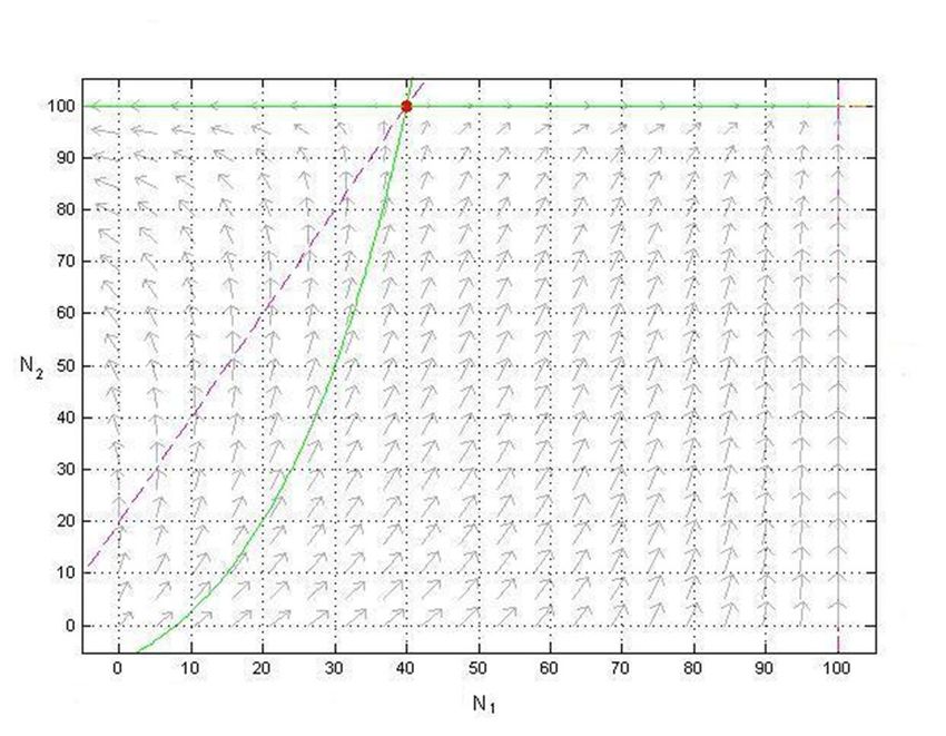
Figure 2 shows a plot of the phase diagram with the separatrix and several sample trajectories
for the following system with 0 ≤ N1 ≤ 100 and 0 ≤ N2 ≤ 100:
dN1
= (0.02 + 0.002N1 − 0.001N2 )(100 − N1 );
dt
dN2
= (0.03 + 0.002N2 + 0.001N1 )(100 − N2 ). (5)
dt
The order of magnitude of the parameters in (5) is consistent with prior research (e.g., Bucklin and
Sengupta 1993; Van den Bulte and Stremersch 2004). For trajectories to the left of the separatrix,
Figure 2 Phase Diagram with Separatrix for the System in (5)
ISOCLINE
SEPARATRIXBakshi, Hosanagar and Van den Bulte: Chase and Flight
Article submitted to Operations Research; manuscript no. 13
the relative size of the installed base in segment 2 to that in segment 1 is so large that the negative
influence exerted by segment 2 dominates segment 1’s growth rate. As a result, the users in segment
1 will eventually disadopt, leading to a final equilibrium outcome (0, m2 ). Conversely, all trajectories
to the right of the separatrix converge to (m1 , m2 ), resulting in full penetration in both segments.
Identifying the stable equilibrium outcomes and the separatrix allows one to answer several
questions. For example, starting from (0, 0), can the system converge to (m1 , m2 )? For the system
in (5), the location of the separatrix in Figure 2 shows that this is impossible.
4.2. Strong Repulsion (Negative LHR1 )
m2 |c1 |−a1
When b1
> m1 , which corresponds to strong repulsive influence by segment 2 on segment1,
the singular point ( m2 |cb11|−a1 , m2 ) is outside the feasible region and thus not of interest. The only
singular point in the feasible region is (m1 , m2 ). A small perturbation of the system around the
singular point (m1 , m2 ) will result in a negative value for dN1 /dt (by virtue of negative LHR1 ),
and thus the trajectory will not return to (m1 , m2 ). This suggests that the singular point (m1 , m2 )
may not be a stable equilibrium point.
The phase diagram for this case can be constructed following the steps described in Section 3,
and is shown in Figure 3. Since N2 0 > 0 for all N2 < m2 , a trajectory starting from any point in
the feasible region will eventually be above the isocline N2 = (a1 + b1 N1 )/|c1 |. Once the trajectory
is above the isocline, we have N1 0 < 0 and N1 decreases until it reaches zero. As a result, the only
possible long-term outcome is (0, m2 ). In the presence of strong repulsion, the long-term outcome
is that the product has no penetration whatsoever in the attractive segment yet full penetration
in the segment that tries to imitate them. This is stated formally in our next result.
Proposition 2. For the Attraction/Repulsion model with a negative value for LHR1 , the only
stable equilibrium outcomes is (0, m2 ) .
Proof: See Appendix A.
4.3. Implications of Equilibrium Analysis
The results show that, in markets with joint attraction and repulsion between segments, the new
product gains full penetration in the repulsive segment, and either zero or full penetration in the
attractive segment. Intermediate levels of penetration cannot be a stable equilibrium. Also, full
penetration in both segments is possible only if the repulsion is sufficiently weak. This confirms
the concerns of managers at companies operating in such markets, like Burberry and Diesel.
Marketing analysts can use the technique described above to identify scenarios in which the
product will achieve its full market potential in both segments or not. If the system parametersBakshi, Hosanagar and Van den Bulte: Chase and Flight
14 Article submitted to Operations Research; manuscript no.
Figure 3 Phase Diagram with Separatrix for Cases with Strong Repulsion
result in a phase diagram as in Figure 3, then full market penetration (m1 , m2 ) will never mate-
rialize. If, in contrast, the situation is as in Figure 2, full-market-penetration is possible but not
guaranteed.
The analysis may also prevent managers becoming lulled in a false sense of security. Consider
the diffusion of the product captured in Figure 3. For a trajectory in the region below the isocline
(where N1 0 < 0), the diffusion within segment 1 may seem to be proceeding quite smoothly early
on, but it will reverse once adoption in segment 2 is sufficiently high. Phase plane analysis may help
protect managers from putting too much faith in early success and believing that the penetration
level will continue to grow.
Finally, the analysis can also be used to identify conditions that managers may want to create in
order to realize the product’s full potential. Lets turn again to Figure 2. A diffusion process that
starts at its “natural” initial state (0, 0) will not reach (m1 , m2 ). Nor will one that starts at (2, 0).
But one that starts at (10, 0) will reach (m1 , m2 ) without any other intervention. So, phase plane
analysis can determine whether or not some initial intervention, such as seeding the process with
initial converts, may actually help achieve full market penetration.
So, equilibrium analysis can help marketing analysts not only determine the extent to which
repulsion is a cause for concern but also assess how strong a marketing intervention is necessary
to steer the process towards full market penetration.Bakshi, Hosanagar and Van den Bulte: Chase and Flight Article submitted to Operations Research; manuscript no. 15 5. Optimal Seeding with Attraction/Repulsion Marketers increasingly try to leverage the power of word-of-mouth to boost the return on their marketing expenditures. As a result, the idea of “seeding” or converting a small number of cus- tomers before launch to help achieve deeper or faster market penetration is currently receiving much attention from marketers. The practice has a long history in the pharmaceutical and med- ical devices industries, and has become popular in consumer goods and services, as reflected in the emergence of “viral-for-hire” companies like BzzAgent, SheSpeaks, and Tremor. Seeding has also become the subject of quite a bit of academic research (e.g., Aral et al. 2011; Bakshy et al. 2011; Berger and Schwartz 2011; Godes and Mayzlin 2009; Goldenberg et al. 2009; Hinz et al. 2011; Iyengar et al. 2011; Jain et al. 1995; Kitsak et al. 2010; Lehmann and Esteban-Bravo 2006; Toubia et al. 2010). While much of this work focuses on identifying the most influential seeding points in network structures more complex than the two-segment work we analyze, research to date has ignored the possibility of attraction/repulsion dynamics between segments. As the results presented here show, the presence of repulsion dynamics can greatly affect not only the optimal level of seeding but even whether one wants to engage in seeding at all. An important consequence of repulsion is that seeding can affect a firm’s profits not only by accelerating the diffusion of the new product but also by affecting the odds of reaching full market penetration. To illustrate, let’s turn again to Figure 2. A diffusion process that starts at its “natural” initial state (0, 0) will not reach full market penetration (m1 , m2 ) but a seeded process starting at any point right of the separatrix, like (10, 0), will. Jain et al. (1995) investigated the optimal seeding level in a single-segment setting and found that optimal levels are high when the coefficient of innovation is low or that of imitation is high. Lehmann and Esteban-Bravo (2006) investigated a two-segment setting with asymmetric attraction (+/0) influence, and found that the optimal seeding in the attractive segment decreases as its coefficient of innovation increases and that it first decreases and then increases as its coefficient of imitation increases. We extend these analyses by investigating optimal seeding for a two-segment setting with attraction/repulsion between the segments. We assume that the product is launched in both segments simultaneously. Seeding occurs in segment 1whose propensity to adopt is impeded by the penetration in segment 2. The purpose of seeding, obviously, is to jump start the process in segment 1 so that its own positive within-segment imitation effect is big enough to withstand the negative repulsion effect. We restrict our analysis to the commonly studied situation where the firm seeds the market only at time 0 and does not intervene with additional seeding later in the diffusion process. The decision problem in a discrete time period analysis is:
Bakshi, Hosanagar and Van den Bulte: Chase and Flight
16                                                                 Article submitted to Operations Research; manuscript no.

                          ∞
                          X                                     ∞
                                                                X
           max π = max          δ t−1 (p1 − u1 )(dN1 /dt)dt +         δ t−1 (p2 − u2 )(dN2 /dt)dt − (s1 N1 S ),        (6)
           N1S      N1S
                          t=1                                   t=1

where π is the net present value (NPV), δ is a discount factor, pi is the price charged to segment i,
ui is the unit cost of manufacturing the product, s1 is the unit cost of generating a seed in segment
1, and N1S is the number of seeded customers in segment 1. This formulation is the same as in Jain
et al. (1995), with the exception that there are two consumer segments in (6). We investigate the
solution numerically using parameters within the same range as those used in Jain et al. (1995).
In order to focus on the impact of repulsion c1 , we assume that c2 = 0. The discount factor is
δ = 1/1.08 = 0.926, and s1 = ui = 0 so pi can be interpreted as profit margin instead of price.
Note that seeding is costly even when s1 = 0, because of the lost revenue p1 N1S from the seeded
customers. We evaluate the value of dN1 /dt and dN2 /dt using the Euler approximation with step
size 1.2 The parameter settings are summarized in Table 2.

                                           Table 2     Parameter Settings
                      Parameter                    Segment 1 Segment 2
                      Innovation (a)                0.005:0.03  0.03
                      Within-segment Contagion (b)     0.002   0.0018
                      Cross-segment Contagion (c)    0:-0.002     0
                      Market Potential (m)              100      100
                      Price (p)                          1        1
                      Unit Cost (u)                      0        0

     Table 3 provides the results for the optimal seeding level for various values of a1 and c1 . The
shaded cells indicate that optimal seeding shifted the equilibrium outcome from (0, m2 ) to full
penetration (m1 , m2 ). For cells to the left of the shaded area, the equilibrium was (m1 , m2 ) without
seeding and remained so after optimal seeding. For cells to the right, the equilibrium remained
(0, m2 ). So, seeding can improve profits both by accelerating diffusion and by shifting the equilib-
rium from zero to full penetration in the attractive segment.
     Reading the table from left to right provides insights into the effect of repulsion on seeding.
For a specific coefficient of innovation (a1 ), the level of optimal seeding initially increases as c1
becomes more negative. This is because more seeding points are needed to help accelerate diffusion
in the face of repulsion. In the shaded area, this acceleration results in a shift of equilibrium to
full penetration. Of particular interest is the decrease in seeding once c1 becomes very negative.
Consider the top right corner of the Table where the optimal level of seeding is nil. When the
attractive segment has a low intrinsic tendency to adopt (low a1 ) and is severely repulsed by the
Bakshi, Hosanagar and Van den Bulte: Chase and Flight
Article submitted to Operations Research; manuscript no. 17
Table 3 Optimal Seeding Levels
c1
Parameters
0 -0.0005 -0.001 -0.0015 -0.002
0.005 6 11 16 26 0
0.006 6 10 16 25 0
0.007 5 10 15 24 0
0.00766 5 9 15 24 0
0.00767 5 9 15 24 21
a1 0.008 5 9 15 24 21
0.009 4 9 14 23 21
0.01 4 8 14 22 21
0.015 1 6 11 19 19
0.02 0 3 8 16 17
0.025 0 1 6 13 15
0.03 0 0 3 10 14
Note: In the shaded cells, optimal seeding shifted the equilibrium outcome from (0, m2 ) to (m1 , m2 ). For cells to the
left of the shaded area, the equilibrium was (m1 , m2 ) both before and after optimal seeding. For cells to the right,
the equilibrium was (0, m2 ) both before and after optimal seeding.
other segment (highly negative c1 ), then effective seeding may become so expensive that the firm
prefers to forego seeding entirely. This explains the zero values in the top right entries in Table 3.
Reading the table from top to bottom provides insights into how the tendency to adopt regardless
of social dynamics (a1 ) affects optimal seeding. For c1 = 0, the optimal seeding levels decrease
with the coefficient of innovation, as reported in Jain et al. (1995). The reason is that seeding is a
substitute for the tendency to adopt spontaneously. The results are qualitatively similar for mild
repulsion, i.e., low negative values of c1 . However, for highly negative values of c1 shown in the
far right column of Table 3, optimal seeding levels may be zero when the coefficient of innovation
is low, then jump quite markedly to a high level beyond a threshold value for the coefficient of
innovation, and finally decline again as the coefficient of innovation increases further. The zero
entries occur because a very large number of seeds may be needed in order to sufficiently accelerate
diffusion when a1 is very small and c1 very negative. As a result, seeding is prohibitively expensive.
However, beyond a certain threshold value for a1 , it becomes profitable to generate seeding points
among consumers in segment 1. In summary, unlike the findings reported in Jain et al. (1995)
in the single segment case and Lehmann and Lehmann and Esteban-Bravo (2006) in the (+/0)
case, optimal seeding need not always decrease with the coefficient of innovation in settings with
negative interaction.
Next, we investigate the impact of the coefficient of within-segment imitation (b1 ) on the optimal
level of seeding. The parameters for the simulation are reported in Table 4 and the results in Table
5. The shaded cells in the latter indicate that optimal seeding shifted the equilibrium outcome from
(0, m2 ) to full penetration (m1 , m2 ). For cells to the left of the shaded area, the equilibrium remained
(m1 , m2 ) regardless of optimal seeding, and for the cells to the right it remained (0, m2 ). HereBakshi, Hosanagar and Van den Bulte: Chase and Flight
18 Article submitted to Operations Research; manuscript no.
again, seeding can improve profits both by accelerating diffusion and by shifting the equilibrium
from zero to full penetration in the attractive segment.
Reading the table from top to bottom shows the impact of within-segment imitation. In the
absence of repulsion (c1 = 0), the optimal seeding level is non-decreasing with the coefficient of
imitation, as reported by Jain et al. (1995). This is because WOM complements seeding: The
higher the imitation, the higher the return obtained from the seeding. However, when there is an
impeding influence from segment 2 (c1 < 0), the optimal number of seeding points is not increasing
but typically decreasing in the coefficient of imitation. This reversal occurs because, the stronger
the endogenous feedback is within the attractive segment, the less the firm needs to engage in costly
seeding to protect the diffusion process within that segment from being harmed by the negative
cross-segment effect. However, there is an exception to this pattern. When the within-segment
imitation is weak but the cross-segment repulsion is strong, which corresponds to the top right area
in Table 5, very large number of seeds may be needed in order to change the equilibrium outcomes.
Such a high level of seeding can be prohibitively expensive, so the optimum is not to use seeding at
all. This result is consistent with the results in Table 3. So, unlike the results reported by Lehmann
and Esteban-Bravo (2006) for the (+/0) case without repulsion, we find that the optimal level
of seeding may be decreasing smoothly, or show abrupt upward jump points followed by smooth
declines, as the coefficient of imitation increases.
Table 4 Parameter Settings
Parameter Product 1 Product 2
Innovation (a) 0.02 0.03
Within-segment Contagion (b) 0.001: 0.005 0.002
Cross-segment Contagion (c) 0:-0.002 0
Market Potential (m) 100 100
Price (p) 1 1
Unit Cost (u) 0 0
Seeding counters the detrimental effect of repulsion and by doing so often shifts the long term
equilibrium. As a result, the optimal level of seeding can be much higher in markets with inter-
segment attraction and repulsion than in markets with homogeneous consumers. For example, Jain
et al. (1995) report that the maximum seeding level observed in their analysis was never higher
than 9%. However, for similar parameters, we find that the maximum seeding levels in the presence
of strong inter-segment interaction can exceed 20%. This is because the role of seeding is not only
to accelerate diffusion, but also to mitigate cross-segment repulsion.Bakshi, Hosanagar and Van den Bulte: Chase and Flight
Article submitted to Operations Research; manuscript no. 19
Table 5 Optimal Seeding Levels
c1
Parameters
0 -0.0005 -0.001 -0.0015 -0.002
0.001 0 7 0 0 0
0.0015 0 4 15 0 0
0.002 0 3 9 17 17
0.0025 0 3 6 10 16
b1 0.003 1 3 5 8 11
0.0035 1 3 4 6 8
0.004 2 3 4 5 6
0.0045 2 3 4 4 5
0.005 2 3 3 4 5
Note: In the shaded cells, optimal seeding shifted the equilibrium outcome from (0, m2 ) to (m1 , m2 ). For cells to the
left of the shaded area, the equilibrium was (m1 , m2 ) both before and after optimal seeding. For cells to the right,
the equilibrium was (0, m2 ) both before and after optimal seeding.
6. Other Policies to Manage Repulsion
As we have shown, seeding can be used to counter the negative effect of repulsion. While this
particular marketing policy is receiving quite a bit of attention, there are also other policies that
can help marketers counter repulsion profitably.
The first policy is to weaken the repulsive effect itself. Decreasing the extent to which success
in the repulsive segment detracts from the product’s appeal in the attractive segment amounts
to making the c2 parameter less negative. Many companies attempt to achieve such “segment
decoupling” by targeting distinct product designs to different segments. Cheaper lines featuring
large brand logos are targeted towards the mass market, whereas expensive designs featuring much
more subtle signals are targeted towards the attractive segment (Berger and Ward 2010; Han et al.
2010). Our analysis suggests two additional policies that could be used effectively.
The second policy is to launch the product sequentially, first in the attractive segment and only
later in the repulsive segment. The idea is similar to that of seeding: Build an early installed base
in the attractive segment that can withstand the negative effect from the other segment. Like
seeding, delaying the launch in segment 2 allows the diffusion process in segment 1 to gain enough
momentum such that it does not get diverted away from full penetration by the repulsion effect.
How entry timing can optimally balance attraction and repulsion in order to avoid disadoption was
already studied by Joshi et al. (2009).
The third policy consists of purposely limiting the market size of the customer segment harming
product adoption in the other segment. This third alternative warrants a bit more discussion,
since it has not been evaluated in the literature. In Section 4.2 we showed that when LHR1 is
negative, the only stable equilibrium outcome is (0, m2 ). In such cases, seeding will not be helpful in
achieving (m1 , m2 ) as a stable outcome. Also, when the repulsive effect is very high, mere productBakshi, Hosanagar and Van den Bulte: Chase and Flight
20 Article submitted to Operations Research; manuscript no.
versioning may not be effective in reducing c2 sufficiently. Limiting the market size of the segment
exerting the negative influence can still be effective in such extreme cases. Restricting m2 to m02 ,
where m02 < m2 , can make (m1 , m02 ) a stable equilibrium outcome that is more attractive than
(0, m2 ). Such a policy can be implemented in several ways, including limiting the distribution of
the product to select channels rarely patronized by the impeding segment. For instance, Diesel
and Burberry have limited the effective access of their products to “wannabes” by restricting
distribution to certain exclusive channels. Such selective distribution is known to be practiced by
other luxury goods retailers as well; see Buettner et al. (2009a,b) for a related discussion and
associated anti-competition concerns. Adding features with no functional utility to the product, or
offering limited editions are other ways to control the availability of the product to the impeding
segment (Amaldoss and Jain 2008).
We now provide a numerical illustration. Table 6 lists the parameter values for the two segments.
The discount factor is set to δ = 0.926. Table 7 reports the results. Segment 2 exerts so much
negative influence on segment 1 that, in the absence of any intervention, the only stable equilibrium
is (0, 100). Reducing the market potential for segment 2 from 100 to 50 increases the total discounted
profit by 22.1% (from 54.42 to 66.46). The new equilibrium is (100, 50) and thus the product reaches
and maintains full penetration in the attractive segment.
Table 6 Parameter Settings
Parameter Segment 1 Segment 2
Innovation (a) 0.02 0.03
Within-segment Contagion (b) 0.003 0.001
Cross-segment Contagion (c) -0.002 0.002
Market Potential (m) 100 100
Price (p) 1 1
Unit Cost (u) 0 0
Table 7 Results for Reduced Market Size
Base Case Demand Control
Market Potential (m2 ) 100 50
Is (m1 , m2 ) stable? No Yes
Profit 54.42 66.46
7. Conclusion
Attraction and repulsion dynamics are quite important for status-oriented products and brands,
and have become of considerable interest to marketing scientists due to recent experimental andBakshi, Hosanagar and Van den Bulte: Chase and Flight Article submitted to Operations Research; manuscript no. 21 empirical evidence (e.g., Amaldoss and Jain 2008; Berger and Heath 2008; Joshi et al. 2009). We present several novel insights about new product growth in such markets. (i) With weak repulsion, the product always gains full penetration in the repulsive segment, but achieves either zero or full penetration in the attractive segment in stable equilibrium. Intermediate levels of penetration are not a stable equilibrium. With strong repulsion, the product always gains full penetration in the repulsive segment and zero penetration in the attractive segment in stable equilibrium. This is a sharper result than that obtained by Miller et al. (1993) in their earlier analysis of attraction and repulsion. It also corroborates marketers’ concerns about the detrimental effect of repulsion. (ii) One can compute separatrices to separate trajectories that converge to different equilibria. Separatrix analysis allows analysts to identify which scenarios will evolve to full penetration in both segments without special managerial intervention. Separatrices can be numerically computed for any system, as described in detail in Appendix B. MATLAB code is available (e.g., Polking and Arnold 2003; http://math.rice.edu/ polking/odesoft/), and the algorithm for computing the separatrix can also be implemented in a spreadsheet. An Excel implementation for the scenario described in section 4.1 is available upon request. (iii) Seeding can be an effective marketing policy to counter the effects of repulsion. (iv) Repulsion affects how the optimal level of seeding in the attractive segment changes with the coefficient of innovation in that segment. In traditional markets without repulsion, it is optimal to decrease seeding when the coefficient of innovation increases, so seeding is a substitute for spon- taneous independent adoption. In markets with repulsion, this does not always hold. Specifically, when the repulsion is very strong, it can be optimal not to engage in any seeding whatsoever even as the coefficient of innovation increases, until it reaches a threshold after which the traditional substitution pattern holds. (v) Repulsion reverses how the optimal level of seeding in the attractive segment changes with the coefficient of imitation. In traditional markets without repulsion, it is optimal to increase seeding when the coefficient of imitation increases, so seeding is a complement to social contagion. In markets with repulsion, the reverse is typically true. Provided the within-segment contagion reaches a minimum threshold, higher contagion implies less rather than more seeding. The reason is that, in markets with repulsion, the benefits of seeding lie less in leveraging contagion to accelerate diffusion than in quickly building an installed base to counter repulsion. Just as with the coefficient of innovation, there is a discontinuity. Specifically, when the repulsion is very strong, it can be optimal not to engage in any seeding whatsoever unless the coefficient of imitation reaches a threshold after which seeding and contagion act as substitutes.
You can also read