Computation of the atmosphere-less light intensity curve during a total solar eclipse by using Lunar Reconnaissance Orbiter topography data and ...
←
→
Page content transcription
If your browser does not render page correctly, please read the page content below
RAA 2021 Vol. 21 No. 1, 11(14pp) doi: 10.1088/1674-4527/21/1/11
 c 2021 National Astronomical Observatories, CAS and IOP Publishing Ltd.                                 Research in
                                                                                                         Astronomy and
http://www.raa-journal.org  http://iopscience.iop.org/raa
                                                                                                         Astrophysics

Computation of the atmosphere-less light intensity curve during a total solar
eclipse by using Lunar Reconnaissance Orbiter topography data and the
DE430 astronomical ephemeris
Yun-Bo Wang1 , Jian-Guo Yan1 , Mao Ye1,3 , Yong-Zhang Yang1 , Fei Li1 and Jean-Pierre Barriot2,1
1
    State Key Laboratory of Information Engineering in Surveying, Mapping and Remote Sensing, Wuhan University,
    Wuhan 430079, China; jgyan@whu.edu.cn, yang.yongzhang@whu.edu.cn
2
    Geodesy Observatory of Tahiti, University of French Polynesia, BP 6570, 98702 Faaa, Tahiti, French Polynesia
3
    Key Laboratory of Lunar and Deep Space Exploration, National Astronomical Observatories, Chinese Academy of
    Sciences, Beijing 100101, China
Received 2020 August 30; accepted 2020 October 27

        Abstract Observations of the sky irradiation intensity in the visible wavelengths during a solar eclipse
        permit to model the Sun diameter, a key number to constrain the internal structure of our star. In this paper,
        we present an algorithm that takes advantage of the precise Moon topography from Lunar Reconnaissance
        Orbiter to compute, with a high resolution in time, the geometrical part (i.e. top-of-atmosphere, and for
        a given wavelength) of the sky irradiation at any given location on the Earth during these events. The
        algorithm is also able to model the Baily’s beads. We give as an application the theoretical computation
        of the light curve corresponding to the solar eclipse observed at Lakeland (Queensland, North Australia)
        on 2012 November 13. The application to real data, with the introduction of atmospheric and instrumental
        passbands, will be considered in a forthcoming paper.

        Key words: eclipse — Moon — Sun: fundamental parameters

1 INTRODUCTION                                                        The history of measuring solar diameter during solar
                                                                 eclipse dates back to the 18th century. The first observation
                                                                 of a solar eclipse to compute the solar diameter was
The solar diameter is a fundamental parameter in solar           conducted in 1715 (Fiala et al. 1994), and a summary of
physics, used to constrain the internal structure of the         measurements of the solar diameter during solar eclipses,
Sun. We refer to Rozelot et al. (2018a) and Sofia et al.         from 1715 to 2010, was written by Adassuriya et al.
(2013) for the relation between solar diameter, solar            (2011). In 1836, the Baily’s beads phenomenon, occurring
luminosity and climate evolution. Due to the fact that the       in total and annular eclipses of the Sun was first recorded
Sun does not have a solid surface, a precise definition of       in writing (Baily 1836). Baily’s beads are caused by the
solar diameter must be agreed upon. We will discuss the          lunar mountains’ deep valleys, and craters at the edge
modern exact meaning later on. Many different methods            of the Moon that break up sunlight (Sigismondi et al.
and instruments have been used to determine the solar            2012). Before Watts published the Watts’ limb charts in
diameter; including meridian circles, Mercury transits,          1963 (Watts 1963), the measurement of the solar diameter
astrolabes, solar diameter monitors, reflecting heliometers      by solar eclipse observation was considered impossible
and the solar eclipses (Thuillier et al. 2005; Rozelot et al.    because the effect of the lunar rugged limb was not
2016; Rozelot et al. 2018a). The Greek astronomer Samos          known well enough. From 1966 to 2010, Watts’ limb
(310 BC — 230 BC) is the earliest astronomer known               charts were widely used in solar eclipse and solar diameter
to have measured the solar diameter by analyzing lunar           measurement research. However, the lunar limb profiles
eclipse observations. He assumed a given diameter for            obtained from the Watts’ limb charts sometimes have
the Earth and determined the solar radius as 900 arcsec          large errors (Soma & Kato 2002). These errors influence
(Thuillier et al. 2005; Rozelot 2006; Rozelot & Damiani          the accuracies of solar diameter measurements; thus, a
2012).
11–2                          Y. Wang et al.: Computation of Light Intensity during Solar Eclipse

high-resolution lunar topography data set is needed. In           Haberreiter et al. (2008) who resolved the long-standing
2009, a global lunar digital elevation model (DEM) data           discrepancy between the seismic and photospheric solar
set with a resolution down to 1/16 degree was produced            radii (Mamajek et al. 2015). We will use this new value
by using the data from the Japanese lunar exploration             (695,700 km) in all the computations done in this paper.
mission SELENE (Araki et al. 2009). This model was used                 In this work, we used the LRO lunar DEM data
by Adassuriya et al. (2011), Sigismondi et al. (2012) and         set to calculate with high accuracy the atmosphere-
Raponi et al. (2012) to determine the solar radius from           less light curve for the solar eclipse observed at
Baily’s beads timing observations. Five years later, the          Lakeland, Queensland (15◦51′ 30′′ S, 144◦ 51′ 20′′ E) on
Lunar Reconnaissance Orbiter (LRO) mission from NASA              2012 November 13. By atmosphere-less, we mean that
published a higher resolution 1/256 degree DEM data               we did not consider the extinction of solar light caused
in 2014. These DEM data are the most accurate lunar               by atmosphere gases and aerosols, the scattering of the
topography data at the time of the writing of these lines.        Sun light by the atmosphere, as well as photometer
                                                                  passbands. We used a pure geometrical optics approach
     It is now time to precise what we mean by “solar
                                                                  (i.e. an “infinite” frequency monochromatic approximation
diameter”. First, this notion implies that the Sun can be
                                                                  for light), taking into account the light-time between Moon
considered as a pure sphere. Our Sun is rotating with a
                                                                  and Earth.
rotation period of 24.47 days at the equator and almost
38 days at the poles. It is argued that there is a 10
km difference between the polar and equatorial diameter           2 DATA AND METHOD
(Rozelot & Damiani 2011; Kuhn et al. 2012; Meftah et al.
2016). No gravity flattening is observed from the tracking        2.1 LRO Digital Elevation Model Data
of Deep Space probes (an upper limit of 2 × 10⁻⁷
was given by Fienga et al. (2011). Within an accuracy             Between July 2009 and July 2013, the Lunar Orbiter
of +/− 10 km, it is therefore justified to use only one           Laser Altimeter (LOLA; Smith et al. 2010), an altimeter
parameter to characterize the Sun “size” (Meftah et al.           instrument onboard the LRO spacecraft (Tooley et al.
2016). Secondly, the Sun limb is not a solid surface, and         2010) gathered more than 6.5 billion laser altimetric
show a progressive darkening, of wavelength-dependent             measurements along ground tracks separated by 1.25 km
character, at its telescopic limit (Hestroffer & Magnan           at the Moon equator with a separation of about 57 m
1998). The most common modern definition is to use a              along-track between laser shots. The diameter of the cross-
wavelength-based approach, such as Lamy et al. (2015)             like laser shot imprint on the Moon surface was about
and Rozelot et al. (2016), where the solar diameter is            50 m for an LRO nominal polar orbit of 50 km altitude.
defined as the value observed at 540 nm optical wavelength        The crossovers between the altimetric tracks on the Moon
(green light). To observe the light-curve at one wavelength       surface were used by the LOLA team to reduce the orbital
implies the use of narrow-band filters, reducing the amount       error of LRO down to a few tens of centimeters. The
of light received by photometers, and so decreases the            average accuracy of each laser shot point after crossover
signal-to-noise ratio. To observe over a wider range              corrections is estimated to be better than 20 meters in
of wavelength improves this ratio, but then a suitable            horizontal position and around 1 meter in Moon radius
average of “wavelength-dependent solar diameters” must            (Mazarico et al. 2012).Thereafter, the calibrated altimetric
be defined (Rozelot et al. 2016). In 2018, the solar radius       measurements were gridded (Digital Elevation Model)
determinations made during the 2012 Venus transit by the          with the algorithm of Wessel et al. (2013) with a resolution
Solar Diameter Imager and Surface Mapper (SODISM)                 of 256 pixels per degree in selenographic latitude
telescope onboard the PICARD spacecraft were published.           and longitude, corresponding to 118 m on the Moon
At 535.7 nm, the solar radius was found equal to 696 134±         equator (Neumann et al. 2011). Gaps between tracks, up
261 km, against 696 156 ± 145 km at 607.1 nm and                  to 4 km at the equator, were filled by interpolation
696 192 ± 247 km at 782.2 nm. It indicates that the solar         (Smith et al. 2010). We downloaded these grid values
radius wavelength dependence on the visible and the               (file “Lunar LRO LOLA Global LDEM 118m” from the
near-infrared wavelength is extremely weak (Meftah et al.         LRO website (see Acknowledgements section). The grid
2018). In 2015, Resolution B3 of the International                values were computed by subtracting the lunar reference
Astronomical Union defined a new value of the nominal             radius of 1737.4 km from the surface radius measurements
wavelength-independent solar radius (695 700 km) that             (Archinal et al. 2011). An improved digital terrain model,
was different from the canonical value used until then            limited to latitudes +/− 60 degrees, exists (Barker et al.
(695 990 km) (Prša et al. 2016). This nominal solar radius       2016) but cannot be used for this work because we need
corresponds to the solar photospheric radius suggested by         the limb from pole to pole.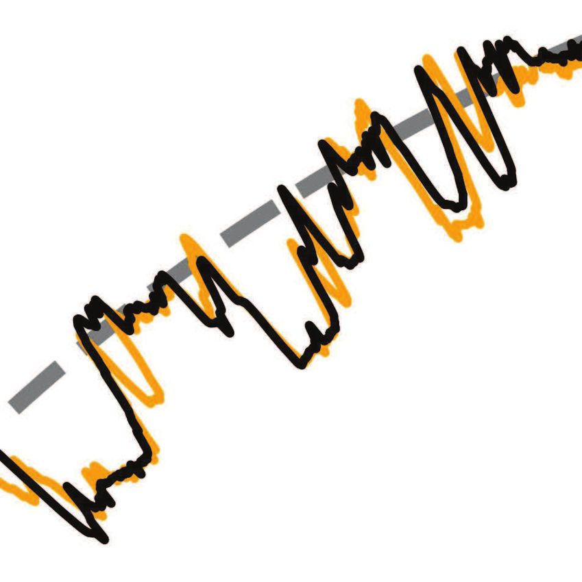
Y. Wang et al.: Computation of Light Intensity during Solar Eclipse 11–3
The latest DE430 ephemeris (Williams et al. 2013; Table 1 Eclipse parameters for the Lakeland (North
Folkner et al. 2014) from the Jet Propulsion Laboratory, Australia) eclipse on 2012 November 13. The eclipse
embedded in the SPICE kernel library (https:// magnitude (*) in the table is the fraction of the Sun’s
naif.jpl.nasa.gov/naif/toolkit.html, ver- diameter obscured by the Moon. The mean radius of the
sion N0066 in our case) was employed to generate the Moon is assumed to be nominally 1737.4 km and the
positions and velocities of the Earth and the Moon. It radius of Sun is nominally fixed at 695 700 km (IAU
is valid from 1549 December 21 to 2650 January 25. resolution 2015-B3). The coordinates of the Sun and the
According to Urban & Kenneth Seidelmann (2013) and Moon were computed from the DE430 ephemeris. The
W.M. Folkner (personal communication, 2020 July 7), geographical coordinates of the observer are: 15◦ 51′ 30′′ S,
the DE430 ephemeris uncertainty in the relative position 144◦51′ 20′′ E.
between the Earth and the Moon is around 1 meter. Calender Date 2012-NOV-13
First Contact (Eclipse Start) 19:44:05 (UTC)
2.2 Observation Model Second Contact (Totality begins) 20:37:38 (UTC)
Mid-Totality Time 20:38:24 (UTC)
2.2.1 Limb geometrical model
Third Contact (Totality ends) 20:39:12 (UTC)
The lunar limb is defined as the lines emanating from the Fourth Contact (Eclipse ends) 21:38:35 (UTC)
observer that are tangent to the Moon. The lunar limb is in Eclipse Magnitude* 1.0375
the “plane of sky”, a plane perpendicular to the direction of Duration of Totality 1 min 34 s
the observer to the center of the Moon. The observational
geometry is given in Figure 1. takes slightly more than one second to cross the Moon-
−−→
As shown in Figure 1, M F and M G are the limb Earth distance, therefore, the OM vector is the solution of
points as seen by the observer, defining a circle in three the equation:
dimensions. M F can be computed by: −−−−−−−−−→
cτ = kO(t)M (c − τ )k (5)
−−→ −−→ −−→
M F = OF − OM (1)
where c is the speed of light, t is the time recorded by the
OM is the vector of observer to the center of the Moon. observer O, τ is the light-time between the point M and
OF is: the point O and k.k is the Euclidean norm. This equation
−−→ is solved iteratively by the SPICE library. The change of
OF = Dµ + r(cos θi + sin θj) (2)
coordinates between the LRO DEM, given in the Moon
−−→
where µ is the unit vector of OM , i and j are two mean equator (MME) frame, and the limb frame is also
orthogonal directions in the plane of sky. i and j can be handled by the SPICE library.
computed by:
2.2.2 Example of limb computation
i=µ×z j =µ×i (3)
We now illustrate the computation of the Moon limb by
where z is the local zenith of the observer. All these using Equations (1)-(5), in the case of the solar eclipse
vectors are functions of time. D is the distance between observed on Lakeland on 2012 November 13 (see Table 1
the observer and the plane of sky and r is the radius of the for details).
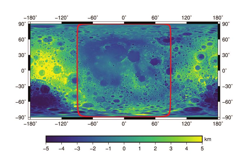
limb profile. D and r are defined by: Figure 2 shows the Moon limb, as seen from the
s observer in Lakeland, plotted on the Moon surface at mid-
2 2
totality.
R R
D =d 1− r =R 1− (4) The limb profiles for both the finite-distance and
d d
infinite-distance observers are shown in Figure 3, enlarged
where d is the distance between the observer and the center by a factor of 40 for legibility.
of the Moon. Figure 4 shows clearly that the infinite-distance
To simplify the problem, a basic assumption could approximation is too crude. The time for the right border
be to assume that the observer is at an infinite distance of the Moon to cross the Sun surface, as seen from the
from the Moon. In this case, we have D=d and r=R, observer at Lakeland, is 3213 seconds (First to Second
and the limb is a great circle on the Moon surface. We contacts, see Table 1). As the mean diameter of the Moon
will see in the next chapter that this assumption is not is 3474.8 km, this means that the velocity of the Moon in
sufficiently accurate. The distances in Equations (1)–(4) the plane-of-sky of the observer is around 1.08 km s−1 ,
have to be understood as “light- time” distances. The light therefore a distance of 770 m is equivalent to 0.713 s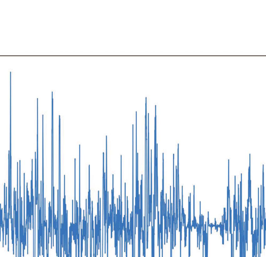
11–4                           Y. Wang et al.: Computation of Light Intensity during Solar Eclipse

Fig. 1 Finite-distance observer model. E is the center of the Earth, O is the observer on the Earth surface and M is the
center of the Moon. The Z direction is the local zenith of the observer. G and F are the limb points as seen from the
observer.

Fig. 2 The Moons limb plotted in the Moon surface, (red line) at 2012-NOV-13 20:38:24 UTC, as observed from Lakeland
on 2012 November 13. The two cases for limb computations (finite -distance and infinite-distance observers) cannot be
distinguished in this figure. The base map is the topographic map from the LRO mission.

in the timing of the Baily’s beads, a totally unacceptable         hours, the duration of the Lakeland eclipse from the first
value, because the timing accuracy for the measurements            to the fourth contacts. As the resolution of the Moon DEM
is typically at the level of 1 millisecond.                        is 1/256 degree, i.e. 108 m at Moon equator, this means
                                                                   that during the two hours eclipse, the limb is displaced
     From a theoretical point-of-view the limb must be             by 25 pixels on the Moon surface (0.1 / (1./.256)). This
recomputed at each observation time, both for the timing           also means that the limb should be recalculated only every
of the Baily’s beads and for light curves, as the Moon rolls       2h / 0.1×(1. / 256.) that is to say around 4 min 30 s.
back and forth around the sub-Earth point as the result            This corresponds to a one pixel displacement caused by
of astronomical forcing (librations, see Rambaux et al.            the diurnal libration for the DEM. As the timing of the
2010). But this comes with a heavy price-tag in terms              Baily’s beads is done during the second and third contacts,
of CPU time. Hopefully, this burden can be reduced to              only separated by 1 min 34 s for the Lakeland example,
a manageable level by considering the resolution of the            this means that we can assume that the limb computation
Moon DEM and the fact that only the daily libration                can be performed only once for this timing. For the whole
amplitude, a small daily oscillation due to Earth’s rotation,      eclipse, we only need to recompute the limb about 25
which carries the observer on Earth first to one side and          times. Our software permits the recomputation of the limb
then to the other side of the straight line joining Earth’s        with any time resolution. The maximum of the differences
and Moon’s centers, is the only one of interests for us.           around totality between a light curve computed with the
Its amplitude is less than one degree (Yang et al. 2017)
in the plane-of-sky. This means about 0.1 degree for two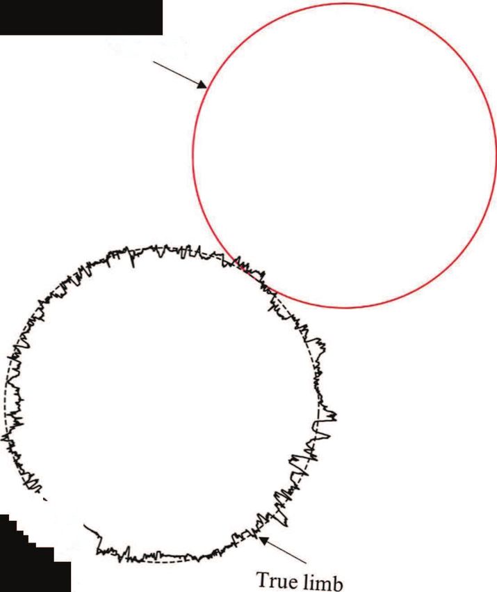
Y. Wang et al.: Computation of Light Intensity during Solar Eclipse                       11–5

Fig. 3 Comparison between the lunar limb as observed from the Earth at a finite distance (orange curve) and the lunar
limb (black curve) observed from an infinite distance along the same line-of-sight. This figure corresponds to the case of
the solar eclipse observed at Lakeland (North Australia) on 2012 November 13. The origin of polar coordinates is dictated
by the local zenith of the observer at the time of the observation (2012-NOV-13 20:38:24 UTC, see Eqs. (1)-(5)).

Fig. 4 Differences between the two lunar profiles plotted in Fig. 3 (finite-distance versus infinite-distance observers). The
average of differences is 770.17 m, the maximum of differences is 6018 m and the standard deviation is 1165.25 m. The
time sampling is 1 s.
11–6                          Y. Wang et al.: Computation of Light Intensity during Solar Eclipse

Fig. 5 Luminous area at 20:20:24 2012-Nov-13. The red area circle is the plane-of-sky illuminated part of the Solar disk
as seen by an observer at Lakeland, the black curve is the Moon limb. UTC time is 20:20:24 2012-Nov-13. The solar
radius is fixed at 695 700 km (Table 1).

limb computed once and the limb computed at each time             3 RESULT
sampling is 2.69 × 10⁻⁶ (Fig. 7(d)).
                                                                  3.1 Light Curve
2.3 Computation of Light Curves                                   Lamy et al. (2015) demonstrated that the modeling of the
                                                                  light curve, in the neighborhood of the second and third
In this section, we compute the geometrical optics approx-        contacts is a powerful way to determine the diameter of
imation of the Sun illumination on Earth surface during           the Sun from ground based photometric curves. Their main
an eclipse. To obtain the light intensity as measured by          argument is that, by observing near the second and third
a photometer on Earth surface, three other parameters are         contacts, the bulk of the solar disk is occulted, resulting in
needed: (a) The (frequency-dependent) extinction of light         very low instrumental and atmospheric levels of stray light
caused by the atmosphere, and especially by its aerosol           (scattered light not coming directly from the Sun). Figure 6
contents; (b) The instrument (convolution) function of the        exhibits the theoretical modeling of such a light curve over
photometer (filters, photodiode characteristics); (c) The         three hours for the Lakeland case.
orientation at any time of the photometer boresight with               The difference in illumination caused by the topog-
respect to the line-of-sight Observer-Moon. This is not           raphy of the Moon is at a level of 0.01 % of the total
treated in this paper, because they are site and instrument       illumination of the unobscured Sun. Figure 6(b) show
dependents. This raw illumination function is defined as          clearly that the left and right parts of the light curve, before
the angular area of the Sun surface not obscured by the           and after the totality, computed from the true limb, are not
Moon. For this purpose, the Moon surface is divided in            symmetrical. This happens because the topography of the
radial triangles, the external part of the triangles being        Moon is highly rugged. The mean radius of the Moon is,
defined by the Moon limb (see Fig. 5). The problem is             as seen from the observer, simply a poor approximation
then to compute the common area between each of these             of the limb. A better approximation of the limb, of course
triangles and the disk of the Sun, and to sum up all the          only strictly valid for the time of the eclipse, would be
triangle contributions. Because the resolution of the LRO         the mean radius of the limb, as seen from the observer.
DEM is 118 m, which is equivalent to 1/256 degree, we             It would be even better to consider two “mean” radiuses,
divided the whole lunar limb in 1/256 degree sub-parts,           the first one corresponding to the half of the Moon limb
obtaining 92 160 small triangles.                                 at play between the first and second contact; and a second
    The mathematics of the computation of the intersec-           one corresponding to the half of the Moon limb at play
tion between a disk and a triangle are not difficult, but         between the third and fourth contacts (Barriot & Prado
tedious, so we discuss them in the Appendix.                      2013). Figure 7(a) shows the light curve from 20:36:00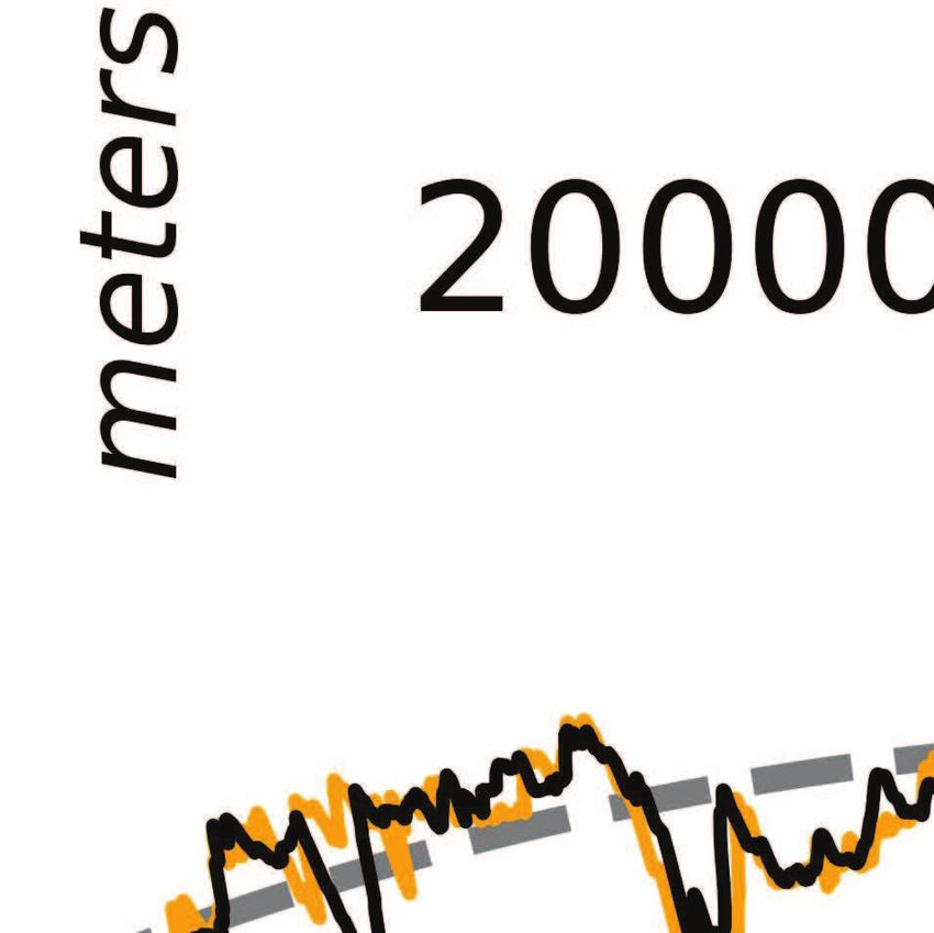
Y. Wang et al.: Computation of Light Intensity during Solar Eclipse                      11–7

Fig. 6 (a) Theoretical light curves for the Lakeland observer (blue: computation with LRO Moon limb, yellow:
computation with the LRO Moon mean radius of 1737.4 km). The radius of the Sun is fixed at 695 700 km (see Table 1)
for the whole 2.5 h eclipse duration, from 2013-Nov-13 19:30:00 to 2013-Nov-13 22:00:00. No difference between the
two light curves can be seen by eye. See Fig. 7(a) for a zoom of the box area. The two light curves (a) and (b) have been
normalized to their maximum values. (b) Differences between the two light curves in the top subfigure 6(a). The time
sampling is 1 s.

to 20:41:00 (total eclipse from 20:37:38 to 20:39:12).            the lunar DEM. These errors were already discussed in
Before the second contact the best fit is obtained for a          Section 2.1: the average accuracy of the DEM grid values
limb “radius” of 1736.85 km, and for a limb radius of             is around 1 meter (Moon radius) and the DE430 ephemeris
1735.55 km after the third contact. This means that the           uncertainty in the relative position between the Earth and
mean topography near the position of third contact is lower       the Moon is also at the level of 1 meter. We estimated
than the mean topography near the second contact (see also        (Fig. 8) the error in the nominal light curve by adding
Fig. 6(b)).                                                       small errors (with plus or minus sign, or zero) at these
                                                                  levels in both the nominal DEM and the nominal Earth-
   Two error sources show up in the light curve                   Moon distance, and making the relative differences in the
computation. The first one is the error contaminating the         corresponding light curves with respect to the nominal
DE430 ephemeris, and the second one is the error on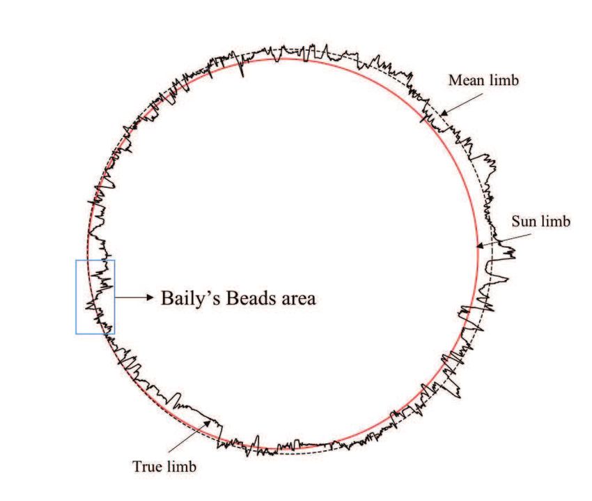
11–8 Y. Wang et al.: Computation of Light Intensity during Solar Eclipse
"
!"
" "
"
"
" " "
"
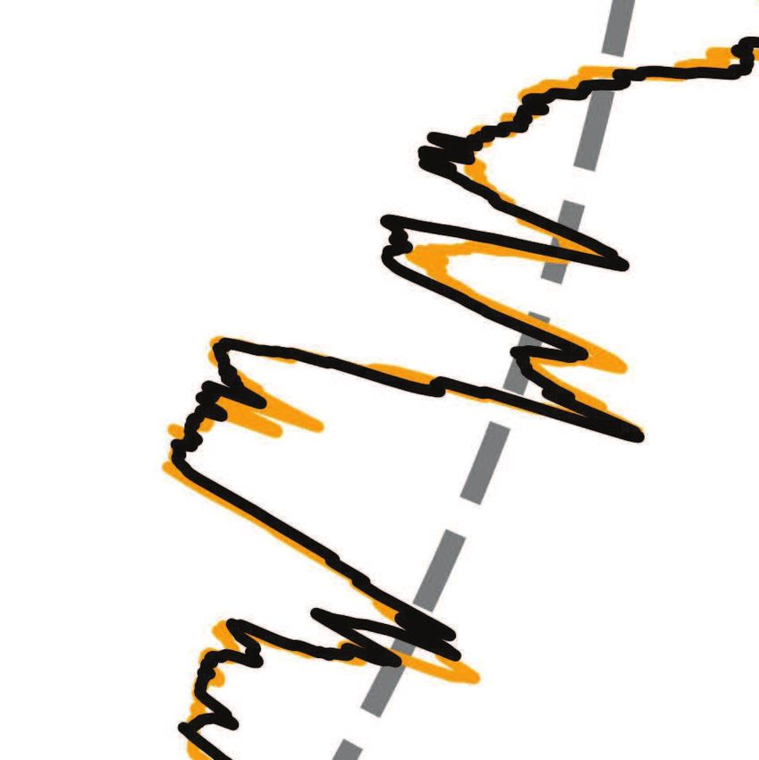
Fig. 7 (a) Light curve “in total eclipse” for a duration of 5 minutes around totality (boxed area in Fig. 6(a)), blue: light-
curve computed from the LRO lunar topography, orange: light-curve computed by considering a disk approximation of
the Moon limb with a radius of 1737.4 km (LRO value), red: light-curve computed by a disk approximation of the Moon
limb with a radius of 1736.85 km corresponding to the mean of the limb topography of 1736.85 km (a good fit for the
second contact, but a poor one for the third contact). (b) Zoom at the time of the second contact, (c) Differences between
the LRO topography light curve during totality (Fig. 7(a)) and the light curve computed with two limbs mean radiuses:
1736.85 km before the second contact and 1735.55 km after the third contact, (d) Difference between the light curves with
the limb computed at each sampling time and the limb only computed once (at mid-totality). The time sampling is 1 s.
light curve. The relative error is dominated, by two orders 3.2 Baily’s Beads
of magnitude, by the DEM error, and ranges between 10−5
and 10−3 at the second and third contacts.
The Baily’s beads, or diamond ring effect, named
The goal of this study is ultimately to show that vari- after Francis Baily, who observed and explained the
ations in the solar diameter can be seen in the photometry phenomenon during the 1836 May 15 solar eclipse seen
curve. The expected variations of solar diameter are at a at Inch Bonney in Scotland, occur when beads of sunlight
level of 400 milliarseconds, corresponding to 145 km in shine through the valleys perpendicular to the Moon limb.
solar radius (Rozelot et al. 2018b). To test this sensitivity, The diamond ring effect is when several beads shine as
we perturbed the solar radius by a 10−6 variation (695 the ring of diamonds of a queen’s crown around the lunar
m), and computed the relative error between the light silhouette. Figure 9 shows the relative position of the Sun
curve with the perturbed solar radius and the nominal light and the Moon at the times of the four contacts as seen
curve (violet curve in Fig. 8). The relative error caused from the observer at Lakeland, and Figure 10 is a snapshot
by the solar radius variation dominates by two orders of of the Baily’s beads evolution during the second contact
magnitude the DEM relative error. As the errors in the (Fig. 9b). The accuracy of the timing of the Baily’s beads
Moon LRO DEM and in the DE430 ephemeris are both at is also dominated by the DEM error, and we estimate
a meter-level scale, this means that, at least theoretically, it to be at the millisecond level (1 m in DEM accuracy
a sensitivity at the level of 100 m in the determination divided by the orbital velocity of the Moon (1 km s−1 ),
of the solar radius can be achieved by our approach. A plus the rotational velocity of the observer on Earth surface
conservative number is certainly around a 1 km accuracy. (4000 km d−1 at the equator).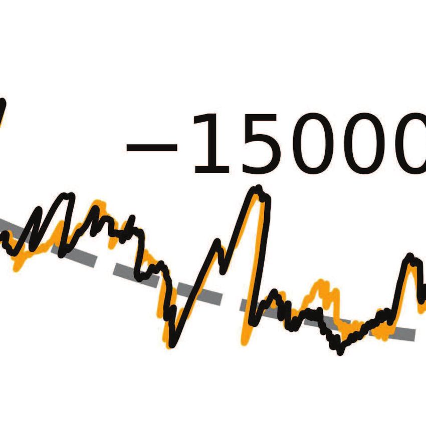
Y. Wang et al.: Computation of Light Intensity during Solar Eclipse                                              11–9


                         4

                         4


                              3%
                                       "$
                                               4

                                                        4 %


                                                               4

                                                                        &   '* ('0!+  ,)  - # !.1 /  2( +


Fig. 8 Estimation of the relative error in the light-curve for the Lakeland observer. The Y axis is the base 10 logarithm
of relative errors. The error settings of the eight cases studied are defined in the label: green: six error curves with a lunar
DEM error, blue: two error curves with a DE430 ephemeris error only, violet: error curve with 10−6 solar radius variation
of the nominal 695 700 km Sun radius value (Table 1). The values of Y are set to zero when the relative errors are zero.
The relative error is dominated, by two orders of magnitude, by the lunar DEM error with respect to the DE430 ephemeris
error. The time sampling is 1 s. The lunar limb was recomputed every 4 min 30 s.

4 CONCLUSIONS                                                                     better than 1 km, and even allow a measurement of solar
                                                                                  oblateness. Using photometers on ground is cheaper but
The observation of solar eclipses is certainly one of the best                    more challenging. The limiting factor is ultimately the
ways to measure the diameter of the Sun, a key parameter                          Earth atmosphere (absorption and scattering). Our next
in the modeling of the inner dynamics of our star.                                work will deal with the Earth atmosphere effect in real data
     In this paper, we focused on the astronomical and                            processing.
astrophysical tools to compute the atmosphere-less part of
this computation, by considering the latest DEM model of                          Acknowledgements This research was supported by
the Moon from the LRO spacecraft and one of the latest                            the National Natural Science Foundation of China
ephemeris of the Earth-Moon system (DE430). Our Python                            (U1831132 and 41804025), grant of Hubei Province
code provides astronomical raw illumination data and tim-                         Natural Science (2018CFA087), also supported by the
ing along the line-of-sight Observer-Center-of-Moon with                          grant from Key Laboratory of Lunar and Deep Space
a millisecond resolution. As an application, we computed                          Exploration, CAS, and LIESMARS Special Research
an atmosphere-less model of the eclipse observed from                             Funding. Planetary ephemerides files can be downloaded
Lakeland in North Australia (15◦ 51′ 30′′ S, 144◦ 51′ 20′′ E)                     from https://naif.jpl.nasa.gov/pub/naif/
on 2012 November 13. Our study demonstrates that a                                JUNO/kernels/spk/(DE430). LRO DEM data can
photometer with a proper calibration of its optoelectronics                       be downloaded from https://pds-geosciences.
and good timing resolution, mounted onboard a spacecraft,                         wustl.edu/lro/lro-l-lola-3-rdr-v1/
can detect variations in the solar diameter with an accuracy                      lrolol_1xxx/data/(ldem_256.jp2).                 Jean-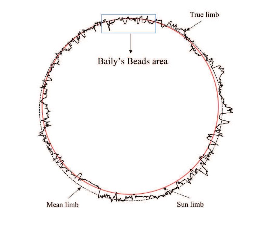
11–10                            Y. Wang et al.: Computation of Light Intensity during Solar Eclipse


                                                             (b) Second contact at 20:37:38
        (a) First contact at 19:44:05

        (c) Third contact at 20:39:12
                                                                   (d) Fourth contact at 21:38:35

Fig. 9 The four contacts between the Moon and the Sun during the Lakeland eclipse. The topography of the Moon has
been enlarged by a factor of 40 to show details. The contact times are defined at the contacts between the circular mean
limb of the Moon and the circular disk of the Sun with a nominal 695 700 km radius (Table 1), not the contacts between
the topography of the Moon and the Sun disk. The boxed areas in Fig. 9(b), Fig. 9(c) are the areas of the Moon concerned
by the apparition of Baily’s beads. Fig. 10(b) shows a zoom of the Baily’s beads during the second contact (Fig. 9(b)).

Pierre Barriot was funded through a DAR grant in                     Case 3: 0 vertices of the triangle in circle, 1 edge intersects
planetology from the French Space Agency (CNES).                     the circle;
                                                                     Case 4: 0 vertices of the triangle in circle, 2 edges intersect
                                                                     the circle;
Appendix A: COMPUTATION OF THE COMMON
                                                                     Case 5: 0 vertices of the triangle in circle, 3 edges intersect
            AREA BETWEEN A TRIANGLE AND
                                                                     the circle;
            A DISK
                                                                     Case 6: 1 vertex of the triangle in circle, 0 edge intersects
In this section, we explored how to compute the                      the circle;
intersection area between a disk and a triangle. Nine cases          Case 7: 1 vertex of the triangle in circle, 1 edge intersects
are listed, as shown in Figure A.1.                                  the circle;
     We obtain nine different cases:                                 Case 8: 2 vertices of the triangle in circle, 0 edge intersects
Case 1: 0 vertices of the triangle in circle, 0 edge intersects      the circle;
the circle (a);                                                      Case 9: 3 vertices of the triangle in circle, 0 edge intersects
Case 2: 0 vertices of the triangle in circle, 0 edge intersects      the circle.
the circle (b);                                                      We adopted different ways to compute the area of
Y. Wang et al.: Computation of Light Intensity during Solar Eclipse 11–11 Fig. 10 Baily’s beads modeled time evolution as seen by the Lakeland observer. White denotes the visible part of Sun. (a) The simulation of Baily’s beads during second contact (from 20:37:18 to 20:37:38, Fig. 9(b)). The time interval between two consecutive pictures is 2 s. (b) The enlargement of the last subplot to show details. Fig. A.1 The nine cases of intersections between a triangle and a circle (adapted from https://stackoverflow.com/questions/540014/compute-the-area-of-intersection-between-a-circle-and-a-triangle).
11–12                              Y. Wang et al.: Computation of Light Intensity during Solar Eclipse

                                                                      (b) case 3.2
            (a) case 3.1

Fig. A.2 The two sub-cases of case 3. (a) case 3.1 the intersection area is the small circular lens, (b) case 3.2 the
intersection area is the large circular lens.

                                                 Fig. A.3 Two parts of intersection.

intersection: For case 1: The intersection area equals the             area of intersection equals the area of the circle minus the
surface of the circle:                                                 area of the circular lens:

                                                                                                                     θ
                           areacase1 = πr2                  (A.1)         areacase3.2 = πr2 − 1/2 θr2 − r cos                (A.5)
                                                                                                                     2
where r is the radius of the circle.                                   where l is the length of the line segment, which intercepts
For case 2:                                                            the circle and r is the radius of the circle. We used
                       areacase2 = 0                        (A.2)      a common strategy to compute the intersection area in
                                                                       case 4, case 5, case 6, case 7, and case 8. As shown in
     For case 3: There are two sub-cases, depending
                                                                       Figure A.3, the area of intersection can be divided into a
whether or not the center of the circle is in the triangle. We
                                                                       polygon and a lens. We computed every partial area and
plotted these two sub-cases in Figure A.2. In Figure A.2,
                                                                       added them up to obtain the area of intersection.
the area of intersection is shown in yellow.
                                                                           The different ways to divide areas of intersection in
     As shown in Figure A.2(a), the center of the circle is
                                                                       cases 4-8 are shown in Figure A.4.
not in the triangle; the area of intersection is the lens shown
                                                                           The area of the polygon in cases 4 through 8 is
in yellow, calculated as:
                                                                       calculated as:

                                             θ                                             1
        areacase3.1 = 1/2 θr2 − r cos                      (A.3)         areapolygon = [(x1 y2 + x2 y3 + x3 y4 + · · · + xn y1 )
                                             2                                             2
                                                                                      − (y1 x2 + y2 x3 + y3 x4 + · · · + yn x1 )]
where is:                                                                                                                      (A.6)
                 areacase3.1 = 2 arcsin(l/2r)               (A.4)      where (xn , yn ) are the coordinates of the vertices of the
and l is the length of the line segment, which intercepts              polygon. The area of the lens can be calculated by:
the circle and r is the radius of the circle. As shown in

                                                                                                                   θ
Figure A.2(b), the center of the circle is in the triangle, the             areacircular lens = 1/2 θr2 − r cos                (A.7)
                                                                                                                   2
Y. Wang et al.: Computation of Light Intensity during Solar Eclipse 11–13
(a) case 4
(b) case 5
(c) case 6
(d) case 7
(e) case 8
Fig. A.4 Different ways to divide the intersection area. (a): case 4, (b): case 5, (c): case 6, (d): case 7 and (e): case 8. The
yellow part is a polygon, the red part is a circular segment (lens).
So, the area of intersection is where s is half the perimeter of the triangle:
areacase4,5,6,7,8 = areapolygon + areacircular lens (A.8) s = 0.5(a + b + c) (A.10)
and where a, b, c are the lengths of the edges of the triangle.
For the case 9 mentioned in Figure A.1: The area of
intersection equals the area of the triangle: References
p
areacase9 = s(s − a)(s − b)(s − c) (A.9) Adassuriya, J., Gunasekera, S., & Samarasinha, N. 2011, Sun and11–14 Y. Wang et al.: Computation of Light Intensity during Solar Eclipse
Geosphere, 6, 17 Rozelot, J. P., & Damiani, C. 2011, European Physical Journal
Araki, H., Tazawa, S., Noda, H., et al. 2009, Science, 323, 897 H, 36, 407
Archinal, B. A., A’Hearn, M. F., Bowell, E., et al. 2011, Celestial Rozelot, J. P., & Damiani, C. 2012, European Physical Journal
Mechanics and Dynamical Astronomy, 109, 101 H, 37, 709
Baily, F. 1836, MNRAS, 4, 15 Rozelot, J.-P., Kosovichev, A., & Kilcik, A. 2016, in Solar
Barker, M. K., Mazarico, E., Neumann, G. A., et al. 2016, Icarus, and Stellar Flares and their Effects on Planets, eds. A. G.
273, 346 Kosovichev, S. L. Hawley, & P. Heinzel, 320, 342
Barriot, J. P., & Prado, J. Y. 2013, in PICARD Third Scientific Rozelot, J. P., Kosovichev, A. G., & Kilcik, A. 2018a, A
Workshop, 25-26 September 2013, CNES Headquarters, Paris Brief History of the Solar Diameter Measurements: a Critical
Fiala, A. D., Dunham, D. W., & Sofia, S. 1994, Sol. Phys., 152, Quality Assessment of the Existing Data, eds. J. P. Rozelot &
97 E. S. Babayev, Variability of the Sun and Sun-Like Stars: from
Fienga, A., Laskar, J., Kuchynka, P., et al. 2011, Celestial
Asteroseismology to Space Weather, 89 (arXiv:1609.02710)
Mechanics and Dynamical Astronomy, 111, 363 Rozelot, J. P., Kosovichev, A. G., & Kilcik, A. 2018b, Sun and
Folkner, W. M., Williams, J. G., Boggs, D. H., Park, R. S., &
Geosphere, 13, 63 (arXiv:1804.06930)
Kuchynka, P. 2014, Interplanetary Network Progress Report, Sigismondi, C., Raponi, A., Bazin, C., & Nugent, R. 2012, in
42-196, 1 International Journal of Modern Physics Conference Series,
Haberreiter, M., Schmutz, W., & Kosovichev, A. G. 2008, ApJL,
12, 405
675, L53 Smith, D. E., Zuber, M. T., Neumann, G. A., et al. 2010,
Hestroffer, D., & Magnan, C. 1998, A&A, 333, 338
Geophys. Res. Lett., 37, L18204
Kuhn, J. R., Bush, R., Emilio, M., & Scholl, I. F. 2012, Science,
Sofia, S., Girard, T. M., Sofia, U. J., et al. 2013, MNRAS, 436,
337, 1638
2151
Lamy, P., Prado, J.-Y., Floyd, O., et al. 2015, Sol. Phys., 290,
Soma, M., & Kato, Y. 2002, Publications of the National
2617
Astronomical Observatory of Japan, 6, 75
Mamajek, E. E., Prsa, A., Torres, G., et al. 2015, arXiv e-prints,
Thuillier, G., Sofia, S., & Haberreiter, M. 2005, Advances in
arXiv:1510.07674
Space Research, 35, 329
Mazarico, E., Rowlands, D. D., Neumann, G. A., et al. 2012,
Tooley, C. R., Houghton, M. B., Saylor, R. S., et al. 2010,
Journal of Geodesy, 86, 193
Space Sci. Rev., 150, 23
Meftah, M., Hauchecorne, A., Bush, R. I., & Irbah, A. 2016,
Urban, S. E., & Kenneth Seidelmann, P. 2013, Explanatory
Advances in Space Research, 58, 1425
supplement to the astronomical almanac (University Science
Meftah, M., Corbard, T., Hauchecorne, A., et al. 2018, A&A,
Books)
616, A64
Watts, C. B. 1963, The marginal zone of the Moon, 17 (US
Neumann, G., Smith, D., Scott, S., Slavney, S., & Grayzek,
Government Printing Office)
E. 2011, National Aeronautics and Space Administration
Wessel, P., Smith, W. H. F., Scharroo, R., Luis, J., & Wobbe, F.
Planetary Data System: http://pds-geosciences.
2013, EOS Transactions, 94, 409
wustl.edu/missions/lro/lola.htm (accessed 20 Williams, J., Boggs, D., & Folkner, W. 2013, DE430 Lunar
August 2015) Orbit, Physical Librations and Surface Coordinates, JPL
Prša, A., Harmanec, P., Torres, G., et al. 2016, AJ, 152, 41
Interoffice Memorandum (Internal Document), Jet Propulsion
Rambaux, N., Castillo-Rogez, J. C., Williams, J. G., &
Laboratory, California Institute of Technology, Pasadena,
Karatekin, Ö. 2010, Geophys. Res. Lett., 37, L04202
California, 19
Raponi, A., Sigismondi, C., Guhl, K., Nugent, R., & Tegtmeier,
Yang, Y.-Z., Li, J.-L., Ping, J.-S., & Hanada, H. 2017,
A. 2012, Sol. Phys., 278, 269
RAA (Research in Astronomy and Astrophysics), 17, 127
Rozelot, J. P. 2006, Advances in Space Research, 37, 1649You can also read