Computer aided autism diagnosis based on visual attention models using eye tracking
←
→
Page content transcription
If your browser does not render page correctly, please read the page content below
www.nature.com/scientificreports
OPEN Computer‑aided autism diagnosis
based on visual attention models
using eye tracking
Jessica S. Oliveira1, Felipe O. Franco2,3, Mirian C. Revers2, Andréia F. Silva2, Joana Portolese2,
Helena Brentani2,3, Ariane Machado‑Lima1,3 & Fátima L. S. Nunes1*
An advantage of using eye tracking for diagnosis is that it is non-invasive and can be performed in
individuals with different functional levels and ages. Computer/aided diagnosis using eye tracking
data is commonly based on eye fixation points in some regions of interest (ROI) in an image. However,
besides the need for every ROI demarcation in each image or video frame used in the experiment,
the diversity of visual features contained in each ROI may compromise the characterization of
visual attention in each group (case or control) and consequent diagnosis accuracy. Although some
approaches use eye tracking signals for aiding diagnosis, it is still a challenge to identify frames of
interest when videos are used as stimuli and to select relevant characteristics extracted from the
videos. This is mainly observed in applications for autism spectrum disorder (ASD) diagnosis. To
address these issues, the present paper proposes: (1) a computational method, integrating concepts
of Visual Attention Model, Image Processing and Artificial Intelligence techniques for learning a model
for each group (case and control) using eye tracking data, and (2) a supervised classifier that, using the
learned models, performs the diagnosis. Although this approach is not disorder-specific, it was tested
in the context of ASD diagnosis, obtaining an average of precision, recall and specificity of 90%, 69%
and 93%, respectively.
Eye tracking is an approach explored by some computational systems to assist in the diagnosis of psychiatric
disorders1,2. An example of disorder that is benefited from the eye tracking technology is the Autism Spectrum
Disorder (ASD), a neurodevelopment disorder characterized by social interaction difficulties, as well as repetitive
behaviors3–5. One of the early signs of ASD is the lack of eye contact4,5. This characteristic can be observed in
toddlers as young as six months of age, regardless of the cultural environment the subject is in. Different stud-
ies, using a specific paradigm, certain regions of interest (ROIs) demarcated on each frame of a video, time and
duration of fixation showed that ASD, compared to controls can be characterized by alterations in early precursor
of social behavior as biological motion, human face preference, and joint attention.
Important results have been achieved using the total duration of gaze fixation in non-biological movements
as a criterion to differentiate the subjects with and without A SD6–10. Pierce et al.9 differentiate groups with 21%
of sensitivity and 98% of specificity. Wan et al10 discriminate groups with 86.5% of sensitivity and 83.8% of speci-
ficity. Shi et al.6 obtained an area under the ROC curve (AUC) of 0.86 with a sample composed of 33 children.
Although, two drawbacks have been described in the ROI-based methods: (1) the need to demarcate each ROI
on each frame of each video used in the experiments, and (2) information waste regarding which visual features
of sub parts of an image had a more fixed gaze. Wang et al.11 showed the importance and contributions of includ-
ing visual attention model (VAM) in ASD’s eye tracking studies.
The importance of image characteristics to VAM have been long recognize. To perform oriented goals,
individuals must specifically allocate their attention, i.e., they must “select” some sensory inputs in detriment
of others, translated as different neuronal firing. This is achieved by integrated bottom-up and top-down brain
circuits. Bottom-up circuits are mostly based on image characteristics such as color, horizontal, vertical and
geometry12. On the other hand, top down systems use an individual prior knowledge13 such as social rules,
concepts learned and experienced selection models of what should be prioritized favoring the individual’s adapt-
ability to the environment14, defined as semantic characteristics. The first computational VAM was developed
by Koch et al.15, based on the Feature Integration Theory (FIT). Visual features such as color, orientation and
1
School of Arts, Sciences and Humanities (EACH), University of Sao Paulo (USP), Sao Paulo, SP 03828‑000,
Brazil. 2Department of Psychiatry, University of Sao Paulo’s School of Medicine (FMUSP), Sao Paulo,
SP 05403‑903, Brazil. 3Interunit PostGraduate Program on Bioinformatics, Institute of Mathematics and Statistics
(IME), University of Sao Paulo (USP), Sao Paulo, SP 05508‑090, Brazil. *email: fatima.nunes@usp.br
Scientific Reports | (2021) 11:10131 | https://doi.org/10.1038/s41598-021-89023-8 1
Vol.:(0123456789)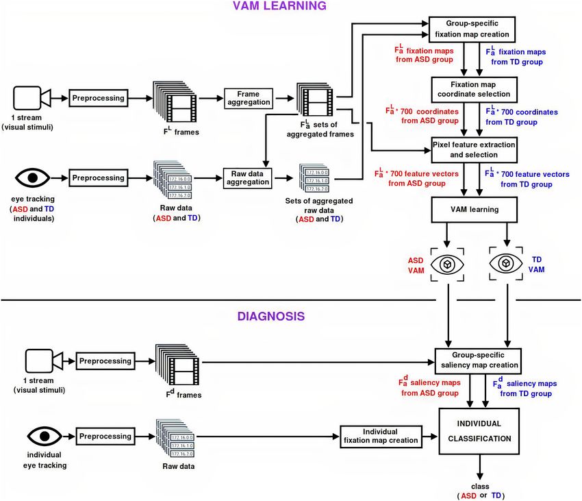
www.nature.com/scientificreports/
Features # of ASD features # of TD features
Steerable pyramids 3 4
Saliency toolbox: color, intensity, orientation and skin 4 4
RGB color 0 1
Horizon line 1 1
Presence of face 1 1
Presence of people 1 1
Distance to the frame center 1 0
Motion value 1 1
Presence of biological movement 1 0
Presence of geometrical movement 1 1
Distance to the side-specific scene center 1 1
Total 15 15
Table 1. Features selected by genetic algorithm for each category.
intensity are extracted from the image of the scene. Then, all the feature maps are combined into a saliency
topographic map. Finally, a cellular network Winner-Take-All is responsible to identify the most conspicuous
location. Thus, processing only the fixation time or the fixation points in a pre-selected area does not allow to
better understand the visual attention standard and its components, as suggested in some previous studies6,11,16.
Itti et al.16 made the first complete computational implementation of the Koch model, creating the most
widely known and used model in the literature. Based on the implementation of Itti et al.16, other approaches
were created, such as Borji et al.17 and Judd et al.18.
The models presented by Borji et al.17 and Judd et al.18 are based on pattern classification. They use super-
vised machine learning methods to learn the VAM using eye tracking data or pixels manually labeled as fixed or
unfixed. Their models use images as inputs and extract around 26 features to form the feature vector used in the
machine learning model. Their features are related to colors, orientation, intensity, steerable pyramids, horizon
line, face, people and distance to the image center.
Approaches based on variations in visual attention standard, can establish different classes of individuals.
Thus, a computational method can use this evidence to classify individuals into such classes. Each class can be
efficiently modeled by a VAM, which can be defined as a description of the observed and/or predicted behavior
of human visual a ttention2,19. Some recent works have been using VAMs to classify individuals using i mages2,20,21.
Duan et al.2 state that VAMs applied to videos can contribute with more discoveries because the videos have
temporal information.
This paper addresses some of the above-mentioned issues by proposing a machine learning approach to
dispense the use of ROIs and develop a classifier based on VAMs learned for each group of individuals: ASD
and Typical Development (TD). The main difference between this paper and those previously cited is the use of
videos as input (instead of static images) to learn VAMs in order to aid ASD diagnosis using eye tracking signals.
Videos can provide a more complete set of observations related to eye tracking but include some challenges to
process. Additionally, our approach offers the possibility of using a video as stimuli for diagnosis different from
that used in the VAM training. This difference represents some challenges for the model construction, whose
solutions are the contributions of the present work. The proposed strategy could contribute not only in case/
control comparison but also in the comparison of two disorders as ASD and Attention-Deficit / Hyperactivity
Disorder (ADHD).
Thus, the main contributions of this paper are:
• an approach to infer two different VAMs—one for ASD individuals and the other for TD individuals—by
using videos as stimuli and considering each group’s most relevant features;
• a technique to group frames of the video stimuli considering movement features;
• a method to classify an individual as ASD or TD, based on its adherence to the two VAMs previously cited,
using any video as stimuli independently of the videos used for the VAM learning.
Results and discussion
Feature selection. Table 1 shows the 15 selected features by applying a Genetic Algorithm on the 28 origi-
nal extracted features. As observed, no Red, Green, Blue color features were selected to classify the ASD visual
attention. On the other hand, the feature related to the image center was only selected by the ASD group patients.
These findings are in agreement with the results found by Wang et al.11, who realized that the ASD group had
a greater focus on the center of the image, even when there was nothing in the center. We also tested the Relief
algorithm to select features. However, the classification performance was worse than that using features selected
by the Genetic Algorithm.
odel22 were selected for both groups, which provides
The features of the Saliency Toolbox related to the Itti m
indications of the biological relevance of such features, i.e., there is evidence that such features are important for
visual attention for all humans in general, regardless of the presence of disorders such as ASD. For the TD group,
the feature related to biological movement was not selected. This fact can be explained by the generic construction
Scientific Reports | (2021) 11:10131 | https://doi.org/10.1038/s41598-021-89023-8 2
Vol:.(1234567890)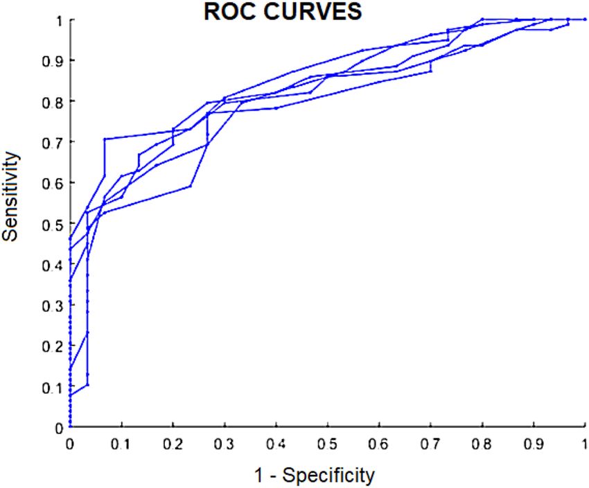
www.nature.com/scientificreports/
Figure 1. ROC Curves for Neural Networks with the features selected by the Genetic Algorithm. The 5 lines
are the results of each of the 5-fold cross-validation rounds (this figure was built with MatLab 2015a version 8.5-
www.mathworks.com/products/matlab.html25).
Classification algorithm Feature selection algorithm Average AUC (standard deviation)
SVM None 0.775 (0.027)
SVM Genetic algorithm 0.695 (0.023)
SVM Relief 0.695 (0.042)
ANN None 0.818 (0.053)
ANN Genetic algorithm 0.822 (0.015)
ANN Relief 0.782 (0.026)
Table 2. Comparison of results of the evaluated approaches.
of the feature, that covers the whole region of the video that presents biological movement. Considering that the
attention of the TD group is specifically more focused on the regions with people and faces (already covered by
the other features), the biological movement does not reveal itself as a discriminant feature to obtain the VAM
of the groups when the cited features set was used.
The features selected by the Genetic Algorithm are plausible with previous studies6,9,11,23,24 in terms of the
relevance of the biological and geometric movement, image center, people and faces in the visual attention of
individuals with ASD.
Classification. Figure 1 shows the ROC curves of the 5-fold cross-validation executions using the proposed
method. Using the Youden method on the ROC curve we obtained a threshold of 28 frames, i.e., an individual
was classified as belonging to the ASD class when 28 or more of her/his fixation maps agreed more with the ASD
than with the TD saliency map. Using this threshold, the average results were 90% of precision, 93% of specific-
ity and 69% of sensitivity/recall . Support Vector Machine (SVM) method was also evaluated as an alternative to
Artificial Neural Networks (ANN) to learn the VAMs. However, the average AUC obtained by using ANN with
Genetic Algorithm was 0.822, while the average AUC using SVM without feature selection was 0.775. In order to
compare the approaches we evaluated, Table 2 presents the average AUC reached with each approach.
In addition to the results obtained, showing the potential of the model itself, an advantage of using eye track-
ing for diagnosis is that it is non-invasive and can be performed in individuals with different functional levels
and ages. Although there are papers that describe the classification of ASD based on eye tracking data6,8,9,26, the
current proposal achieved this classification with AUC higher than most of the projects cited (Table 3), also using
a heterogeneous dataset in terms of age, gender and CARS. In addition, analysis using VAMs avoids the need to
demarcate regions of interest by a specialist, which can lead to data loss and bias.
Several pro-cess steps have been modified from previous m odels17,18 to obtain better results, therefore they
constitute contributions as well as topics for future research: an example is the grouping of frames using motion
information, the pixel selection strategy, feature selection, similarity calculation and the classification process
itself.
The classification proposal based on visual attention utilizing the above mentioned steps is innovative, not
previously found in the literature. In addition to the entire proposed method for aiding ASD diagnosis, which
Scientific Reports | (2021) 11:10131 | https://doi.org/10.1038/s41598-021-89023-8 3
Vol.:(0123456789)www.nature.com/scientificreports/
Reference Dataset Average AUC
Chevallier et al.26 81 children (6–17 years) 0.71
Pierce et al.9 334 children (1–3 years) 0.71
Shi et al.6 33 children (4–6 years) 0.86
This work 106 children (3–18 years) 0.82
Table 3. Comparison of results among related work.
presented promising results for the health area, the pipeline here defined constitutes a basis that can be reused
or adapted to solve similar problems (where the attention can be indicative of the presence of the disorder) by
computational approaches.
Finally, our approach can be applied using other visual stimuli, provided it is possible to extract the same
features used. In addition, different stimuli can be used for VAM training and individual classification. This allows
more flexibility to researchers of the health area and avoids the need of a database with specific stimuli. In the
testing of the present article, we used the same videos for training and testing. Although it could be interpreted
as contamination and biasing of learning, to circumvent this issue we did not use all the pixels in the VAM
Learning phase. As described in section “Fixation map coordinate selection”, we select the 350 coordinates with
the highest values to represent pixels of class 1 (related to fixations) and we also randomly select 350 pixels with
zero fixation value to represent the class 0 (in which there was no fixation). We believe that this random selection
approximates a scenario of usage of different videos, as long as these new videos use the same stimulus paradigm
and have similar characteristics those used in this paper.
The approach presented in this paper processes eye tracking data to learn a supervised classifier based on
VAMs. This approach achieved high performance (average precision of 90%) to classify individuals as belonging
to the ASD or TD groups. Besides the social impact of the method, our approach offers a computational model
that can be extended to be used as a tool for computer-based diagnosis of other disorders where the visual atten-
tion change is indicative of the presence of illness.
The method also brings some advances and presents research opportunities for the area of visual computing,
since it presents different approaches in several stages of the developed method, such as: grouping of frames,
selection of pixels, method of comparison between the fixation map and the saliency map, independence of
stimuli, and the classification method itself.
A challenge to be overcome in this area is composing a robust dataset, since obtaining eye tracking signals
with the respective evaluation of experts is not a trivial task. Thus, we intend to continue our dataset formation
in order to make it available for the scientific community. We also intend to evaluate other machine learning
techniques as well as to extract additional features, both aimed at improving the performance of the proposed
approach.
Material and methods
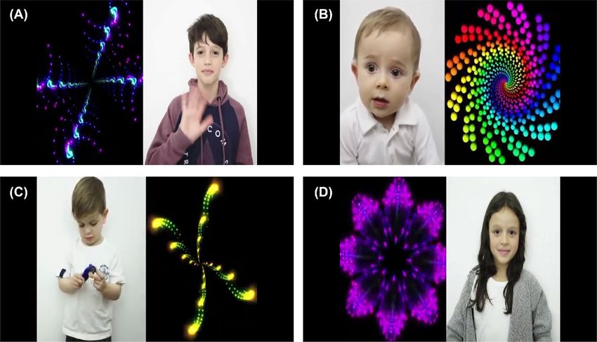
Figure 2 summarizes the entire method developed to classify a subject into ASD or TD class, composed of two
phases: VAM learning and Diagnosis. The method considers two types of input data—a video used as stimulus
and signals captured from an eye tracking—, which will be described in sections “Stimuli” and “Preprocessing”.
The VAM learning phase is responsible to process both the video used as stimulus and the eye tracking signals
from the two groups (ASD and TD) to obtain a VAM model for each group. The frames of the video used as
stimulus are submitted to a preprocessing step followed by a frame aggregation process. Similarly, the eye track-
ing signals are submitted to a preprocessing step followed by an aggregation process that follows the respective
frame aggregations. The sets of aggregated frames and the sets of aggregated raw data are used together in the
next steps: Group-specific fixation map creation, Fixation map coordinate selection, Pixel feature extraction
and selection, and, finally the VAM learning. These eight steps are detailed in the subsections of section “VAM
learning phase”. The Preprocessing step is described only once (since it is similar for both frames and raw data.
Similarly, aggregation of frames and raw data is described together in the section “Frame and raw data aggrega-
tion”, also because the processing for both data types are the same.
The Diagnosis phase receive the same data from the first phase (video used as stimulus and eye tracking
signals, not necessarily from the same stimulus used in the VAM learning phase) and, in addition, the learned
ASD and TD VAMs. However, here the eye tracking signals are related to only an individual, who will be classi-
fied as belonging as ASD or TD class. For this, three steps are necessary: Group-specific saliency map creation,
Individual fixation map creation, and, finally, individual classification. These three steps are detailed in the
subsections of section “Diagnosis phase”.
It is important to highlight that, in the method evaluation, no information of subjects used for testing (“Diag-
nosis phase”) is used in the learning phase, once the cross-validation was performed over the subjects.
Data acquisition. Ethical approval. The present study was approved by the Ethics Committee of the Uni-
versity of São Paulo, Brazil (protocol 57185516.9.0000.5390). All participants or their legal guardians signed an
informed consent.
All procedures performed in this study, that involves human participants were in accordance with the ethical
standards of the institutional and national research committee and with the 1964 Helsinki Declaration and its
later amendments or comparable ethical standards.
Scientific Reports | (2021) 11:10131 | https://doi.org/10.1038/s41598-021-89023-8 4
Vol:.(1234567890)www.nature.com/scientificreports/
Figure 2. Overview of the entire process of the proposed model (this figure was built with XPaint version
2.9.10- https://directory.fsf.org/wiki/Xpaint27).
The informed consent for publication of identifying information/images in an online open-access publication
was obtained from the video participants.
Equipment and subjects. The eye tracking data was acquired using a Tobii Pro TX300 equipment28. Data from
106 subjects were collected to develop the model: 30 from the TD group (10 females and 20 males), and 76 from
the ASD group (27 females and 49 males) All participants have age ranging from 3 to 18 years old.
The ASD subjects were recruited from the Psychiatry Institute, University of São Paulo School of Medicine
(IPq-FMUSP), Brazil. The diagnoses were made based on the subject’s clinical evaluation by a child psychia-
trist using the DSM-V (Diagnostic and Statistical Manual of Mental Disorders) criteria3 and ASD severity was
measured using the Childhood Autism Rating Scale (CARS)29. CARS was also applied in TD subjects to confirm
that they were out of the spectrum, with results below 30 points. Functional cognitive evaluation was performed
by a trained neuropsychologist, using Wechsler Intelligence Scale for Children (WISC)30, Repetitive Behavior
Scale (RBS)31, Vineland Adaptive Behavior S cales32 when possible. All clinical information of ASD individuals
is available in Supplementary Material (Table S1).
ASD is a heterogeneous neurodevelopmental disorder and commonly co-occurs with other conditions such
as psychiatric or neurological d isorders33. Comorbidities vary according to different ages. Some comorbidities
as Anxiety could be detected in 30-50% of ASD patients and attention-deficit/hyperactivity disorder (ADHD)
in 40% of ASD infants34. Together with core symptoms, co-occurring emotional and behavioral problems are
very often present and contribute to different ASD trajectories35,36. Considering these findings, individuals with
comorbidities were not excluded from our study.
Scientific Reports | (2021) 11:10131 | https://doi.org/10.1038/s41598-021-89023-8 5
Vol.:(0123456789)www.nature.com/scientificreports/
Figure 3. Example of frames of the video used as visual stimuli for training the Visual Attention Models (this
figure was built in XPaint version 2.9.10- https://directory.fsf.org/wiki/Xpaint27).
Stimuli. The visual stimuli for training the VAMs were built with the collaboration of experts. They consist of
videos of about 6 s each, where each frame has spatial resolution of 1920 × 1080 pixels. In each video the com-
puter screen was divided into two parts: one with biological movements, which presents the children’s interac-
tions with each other, and another with geometric movements, which presents fractal movements.
Three videos with biological movements and three with geometric movements were combined, composing
nine videos displayed sequentially, with total time of 54 s. Figure 3 presents some frames of the stimuli. The order
and position of figures with biological and geometric movements are changed throughout the video in order to
avoid conditioning of the subjects.
Protocol. A data acquisition protocol was defined, composed of three steps: participant positioning, equipment
calibration and data acquisition.
In the first step, the subject was seated at a distance between 50 and 70 cm from the eye tracking monitor.
With the subject in a suitable position, a five-point eye tracking calibration was used. It shows an animated
image at five different points on the screen. The subject was asked to follow the image with his/her gaze. Thus,
the eye tracking device was able to recognize the eye position. In case of failure, the calibration was repeated. In
case of a second failure, the subject was excluded from the experiment.
The acquisition was started after the calibration. During the entire session, an expert or caregiver was respon-
sible for ensuring that the subject would remain seated and with his attention on the screen. Depending on the
subject’s height it was necessary to sit him/her on the lap of an adult. In these cases, the adult used a blindfold in
order to avoid influencing the signals acquired. All selected subjects had more than 80% of the total video time
captured by the eye tracking equipment.
Proposed method. The next subsections detail each step of the method presented in Fig. 2.
VAM learning phase. This section describes how the ASD and TD VAMs were learned. Each model is a binary
classifier that given a pixel, with a set of features, it will output if this pixel will be fixed by the subject of a specific
group or not.
Therefore, the objects used in the learning process of such models are the pixels that arise from the video
processing, each one represented by a feature vector, described as follows. The classes considered were 1 (pixel
was fixed) and 0 (pixel was not fixed).
Preprocessing. Initially the visual stimuli, which are in video format as previously described, were divided into
frames. Then, a preprocessing was performed in each frame, which consisted of: removing the edges around the
frame (black background, as can be seen in Fig. 3), resizing the frames to a resolution of 200 × 350 pixels and
removing the transition frames between two videos (ten last frames of a video and ten first frames of the follow-
Scientific Reports | (2021) 11:10131 | https://doi.org/10.1038/s41598-021-89023-8 6
Vol:.(1234567890)www.nature.com/scientificreports/
Figure 4. Example of fixation maps for a video frame that contains a scene of biological movement on the left
side and a scene of geometric movement on the right side. The frame used for generating these maps are similar
to frames B and C in Fig. 3 (this figure was built with MatLab 2015a version 8.5-www.mathworks.com/products/
matlab.html25).
ing video). In Fig. 2, F L is the number of frames that resulted from this process in this phase of VAM learning.
The raw data provided by the eye tracker (pixel coordinates and timestamp) from ASD and TD individuals were
also preprocessed in order to correspond to the same frames and regions.
Frame and raw data aggregation. The basis for the VAM learning is the information regarding which pixels
were fixed by the subjects and which pixels were not. However, once the stimuli are videos, each single frame
does not have enough fixation points to extract information. To circumvent this problem, we aggregated con-
secutive frames with a mean motion value among them of less than 0.33.
The concept of optical flow was used to compute the mean motion value. It is calculated by comparing a frame
with the next one and returning a value of movement for each pixel. This value takes into consideration mainly
the difference in intensity of a pixel in the current frame compared to the correspondent pixel in the next frame37.
For the current frame, we sum all the values of motion of each pixel compared to the respective pixel in the next
frame. Then, we divide the result by the total of pixels (7000). The final motion value is in interval [0 − 1]. If the
final value is lower than 0.33 we aggregate the features and the frames themselves. corrFor this, the feature vector
of each pixel of this frame aggregation consists of the mean value of the original values of the respective pixels.
The resultant frame aggregation is compared to the next frame in order to verify if a new aggregation should
be performed or not. The threshold was defined by analyzing visually the video used as stimulus to identify
when images of two consecutive frames were nearly the same. We identified the average value of movement that
allowed us to group consecutive frames whose variation in the pixels could indicate that no or little movement
was detected. Using optical flow showed itself an efficient approach to do this task automatically. This value is
directly related to the video. Thus, in case of using a different video, this value should be reviewed.
In Fig. 2, FaL is the number of sets of aggregated frames that resulted from this process ( FaL < F L ). For each
set of aggregated frames, the corresponding raw data were also aggregated.
Creation of group‑specific fixation map. The sets of aggregated raw data from each group were used to create
FaL group-specific fixation maps. A fixation map is a matrix, with the same size of frames that compose the corre-
sponding set of aggregated frames. Each position of this matrix has the number of gaze fixations in the respective
coordinate. For each set of aggregated frames, two group-specific fixation maps were created summing up the
number of fixations on the frames of all the subjects from a group (ASD or TD). In each map a Gaussian filter,
with a kernel of size 5x5, was applied to smooth the fixations. This procedure generates a gray-level image that
represents the fixation map where clearer cells indicate the positions that were most fixed by the group (Fig. 4).
Scientific Reports | (2021) 11:10131 | https://doi.org/10.1038/s41598-021-89023-8 7
Vol.:(0123456789)www.nature.com/scientificreports/
Fixation map coordinate selection. The remaining processes of this phase aim to create the pixel feature vectors
that will be used to train the ASD and TD models. These models are binary classifiers able to predict if a pixel will
be fixed or not by the specific group, considering its features (section “Pixel feature extraction and selection”).
The role of the fixation map coordinate selection is to define a balanced training sample for this purpose.
For each group-specific fixation map, the 350 coordinates with the highest values were selected to create
the representative pixels of class 1 (in which there were fixations) and 350 pixels with zero fixation value were
randomly selected as representative pixels of class 0 (in which there was no fixation). This process generated 700
coordinates for each fixation map from, summing up FaL ∗ 700 coordinates for each group.
Pixel feature extraction and selection. The pixel feature extraction process is responsible for creating the 700
feature vectors from each group-specific fixation map, generating a total of 2 ∗ FaL ∗ 700 feature vectors. For
each coordinate selected in the previous process (section “Fixation map coordinate selection”), the respective
feature vector was composed of 28 features, each feature derived from all pixels presented in that coordinate in
the aggregated frames corresponding to that group-specific fixation map. More specifically, each feature value
of a specific coordinate was calculated by averaging the feature values of the pixels from the aggregated frames
in that coordinate.
These 28 features were chosen based on the models most cited in the literature17,18. These models have defined
the features considering studies on Biology and Psychology areas related to human visual attention. Moreover,
some of these features, related to the face, presence of people and movement, are also relevant to the typical
visual attention observed in individuals who belong to the ASD spectrum. We used the following features: 13
steerable pyramids with four scales and three orientations38; color, intensity, orientation, and the presence of
skin (these four features were generated by the Saliency Toolbox39), three features representing the RGB (Red-
Green-Blue) color channels; a feature indicating the presence of horizon line18,40 that was detected by using a
mixture of linear regression trained with “gist” descriptor (a representation of an image in low dimension with
information of the s cene41); two features regarding the presence of faces and people, r espectively42; one feature
regarding the Euclidean distance from the current pixel to the central pixel of the screen and another feature
with the Euclidean distance from the current pixel to the central pixel of the scene (the scene corresponds to the
half of the screen where the current pixel is located); a feature indicating the amount of movement, calculated
ow37 (detailed in the section “Frame and raw data aggregation”); and the last two binary features
by optical fl
indicating if the current pixel belongs to a biological or geometric scene.
After extracting the above mentioned features, we used a Genetic A lgorithm43 to select the best features in
distinguishing pixels from classes 0 and 1 for each group. The 15 best features (shown in section “Feature selec-
tion”) compose the feature vector used in the learning process of the VAM of each group.
VAM learning process. The 2 ∗ FaL ∗ 700 feature vectors resulting from the previous process were used for
learning the ASD and TD VAMs. For this learning we used a neural network with ten neurons in a single hid-
den layer and stop condition to achieve 1000 training cycles or error less than 1e−7. We used the binary cross-
entropy as loss function, stochastic gradient descent as optimizer and a learning rate of 0.01. The activation func-
tions were the sigmoid in the hidden layer and linear in the output layer. Each learned neural network (ASD or
TD VAMs) is able to predict if a specific pixel, represented by its 15-feature vector, will be fixated by an individual
from its specific group (ASD or TD) or not.
Diagnosis phase. This section describes how the ASD and TD VAMs were used in the diagnosis phase. The
videos containing the stimuli used in this phase are independent from the videos used for the VAMs learning,
which is a differential of our proposal. Since we work with features extracted from the pixels, which are used to
learn the VAMs, any video with similar characteristics that we used (i.e., containing geometric and biological
movement) can be used in this diagnosis phase. When different videos are used, they need to be preprocessed
in the same way as the videos used for learning (section “Preprocessing”), generating F d frames for diagnosis. In
this work we used the same stimuli, but with different frames for the learning and diagnosis phases, as described
in section “Individual classification”.
Group‑specific saliency map creation. A saliency map is a matrix, with the same dimension of the frame that
contains in position (i, j) the probability of the pixel (i, j) of the frame to be fixed. However, our goal is to obtain
binary saliency maps (in which each position is a 0 or 1 value) to compare them to the individual fixation maps
(section “Individual fixation map creation”). Then, the ASD and TD VAMs, learned as described in the last sec-
tion, can be applied in any stimuli to generate a corresponding binary saliency map based on the features of the
frame pixels.
In this work, the two VAMs (ASD and TD) were applied to each pixel of each diagnosis frame, generating F d
ASD binary saliency maps and F d TD binary saliency maps. Thus, the saliency map of a set of aggregated frames
is a matrix where each position has a value 1, indicating the prediction that the respective pixel will be fixed by
an individual of that group, or 0 otherwise.
Individual fixation map creation. In this step, the raw data captured by the eye tracker from the individual
being analyzed is used to create a fixation map for each diagnosis frame. The fixation map of the subject is a
matrix containing 0 in the positions related to the pixels that were not fixed and 1 in the positions of the pixels
that were fixed by that subject. The procedure executed in this step generates F d fixation maps from that indi-
vidual.
Scientific Reports | (2021) 11:10131 | https://doi.org/10.1038/s41598-021-89023-8 8
Vol:.(1234567890)www.nature.com/scientificreports/
Individual classification. The classification process is responsible for answering to which group the individual
belongs: ASD or TD. For this, the F d individual fixation maps (section “Individual fixation map creation”) are
compared with the F d binary saliency maps from both groups.
For each diagnosis frame, the subject’s fixation map was compared to the binary saliency map generated for
each group (section “Saliency map creation”). Given a position (i, j), a match occurs when the individual fixa-
tion map and the binary saliency map have the same value in this position or, in other words, when the model
correctly predicts whether the pixel will or will not be fixed by that individual. That way, the number of matches
between the two maps (individual and group) is considered a measure of similarity between them. The group
of the saliency map (ASD or TD) that was most similar to the subject’s fixation map receives one vote to classify
the subject.
As previously mentioned, our approach allows using any video for the diagnosis phase. In this work, instead
of using different stimuli in the diagnosis phase, we used the same video. However, in order to simulate a differ-
ent video, F d = 50 frames from the original stimuli videos were removed from the VAM learning and used for
this diagnosis phase. Each possible threshold of ASD votes needed to classify an individual to the ASD group
leads to different classification performance measures, such as sensitivity and specificity. Then, a ROC (Receiver
Operating Characteristic) curve can be created varying these threshold values.
The entire process (VAM learning and diagnosis, described in sections “VAM learning phase” and “Diagnosis
phase” ) was repeated using a 5-fold cross-validation for the subjects. In each fold, the diagnosis phase was per-
formed using data from 20% of the subjects and 50 diagnosis frames from the original stimuli video (composed
of F L + F d frames), whereas the VAM learning was performed using the remaining subjects and frames. Also, we
used the ROC curve to apply the Y ouden44 method in order to calculate the best threshold of votes. The results
of the five folds indicated that, from 50 diagnosis frames, the suitable threshold was 28 ASD votes to classify an
individual to the ASD group.
Received: 25 November 2020; Accepted: 24 March 2021
References
1. Beltrán, J.; García-Vázquez, M.S.; Benois-Pineau, J.; Gutierrez-Robledo, L.M.; Dartigues, J.-F.: Computational techniques for eye
movements analysis towards supporting early diagnosis of Alzheimer’s disease: a review. Comput. Math. Methods Med. 2018,
1–13 (2018). https://doi.org/10.1155/2018/2676409
2. Duan, H., et al.: Visual attention analysis and prediction on human faces for children with autism spectrum disorder. ACM Trans.
Multimed. Comput. Commun. Appl.(TOMM) 15, 1–23 (2019). https://doi.org/10.1145/3337066
3. Association, A.P.: Diagnostic and statistical manual of mental disorders, 5th edn. American Psychiatric Association Publishing,
USA (2013)
4. Apicella, F.; Costanzo, V.; Purpura, G.: Are early visual behavior impairments involved in the onset of autism spectrum disorders?
Insights for early diagnosis and intervention. Eur. J. Pediatr. 179, 1–10 (2020). https://doi.org/10.1007/s00431-019-03562-x
5. Franchini, M.; Armstrong, V.L.; Schaer, M.; Smith, I.M.: Initiation of joint attention and related visual attention processes in infants
with autism spectrum disorder: literature review. Child Neuropsychol. 25, 287–317 (2019). https://d oi.o
rg/1 0.1 080/0 92970 49.2 018.
1490706
6. Shi, L., et al.: Different visual preference patterns in response to simple and complex dynamic social stimuli in preschool-aged
children with autism spectrum disorders. PLoS ONE 10, 1–16 (2015). https://doi.org/10.1371/journal.pone.0122280
7. Moore, A., et al.: The geometric preference subtype in ASD: Identifying a consistent, early-emerging phenomenon through eye
tracking. Mol. Autism 9, 19 (2018). https://doi.org/10.1186/s13229-018-0202-z
8. Pierce, K.; Conant, D.; Hazin, R.; Stoner, R.; Desmond, J.: Preference for geometric patterns early in life as a risk factor for autism.
Arch. Gen. Psychiatry 68, 101–109 (2011). https://doi.org/10.1001/archgenpsychiatr y.2010.113
9. Pierce, K., et al.: Eye tracking reveals abnormal visual preference for geometric images as an early biomarker of an autism spectrum
disorder subtype associated with increased symptom severity. Biol. Psychiatry (2015). https://doi.org/10.1016/j.biopsych.2015.03.
032
10. Wan, G., et al.: Applying eye tracking to identify autism spectrum disorder in children. J. Autism Dev. Disord. 49, 209–215 (2019).
https://doi.org/10.1007/s10803-018-3690-y
11. Wang, S., et al.: Atypical visual saliency in autism spectrum disorder quantified through model-based eye tracking. Neuron 88,
604–616 (2015). https://doi.org/10.1016/j.neuron.2015.09.042
12. Hosseinkhani, J.; Joslin, C.: Saliency priority of individual bottom-up attributes in designing visual attention models. Int. J. Softw.
Sci. Comput. Intell. (IJSSCI) 10, 1–18 (2018). https://doi.org/10.4018/IJSSCI.2018100101
13. Katsuki, F.; Constantinidis, C.: Bottom-up and top-down attention: Different processes and overlapping neural systems. Neuro-
scientist 20, 509–521 (2014). https://doi.org/10.1177/1073858413514136
14. Ma, K.-T. et al. Multi-layer linear model for top-down modulation of visual attention in natural egocentric vision. In 2017 IEEE
International Conference on Image Processing (ICIP), 3470–3474. https://doi.org/10.1109/ICIP.2017.8296927 (IEEE, 2017).
15. Koch, C.; Ullman, S.: Shifts in selective visual attention: towards the underlying neural circuitry, Vol. 188. Springer, Berlin (1987)
16. Itti, L.; Koch, C.; Niebur, E.: A model of saliency-based visual attention for rapid scene analysis. IEEE Trans. Pattern Anal. Mach.
Intell. 20, 1254–1259 (1998). https://doi.org/10.1109/34.730558
17. Borji, A. Boosting bottom-up and top-down visual features for saliency estimation. In Computer Vision and Pattern Recognition
(CVPR), 2012 IEEE Conference, 438–445, https://doi.org/10.1109/CVPR.2012.6247706 (IEEE, 2012).
18. Judd, T., Ehinger, K., Durand, F. & Torralba, A. Learning to predict where humans look. In Computer Vision, 2009 IEEE 12th
international conference, 2106–2113, https://doi.org/10.1109/ICCV.2009.5459462 (IEEE, 2009).
19. Tsotsos, J.K.; Rothenstein, A.: Computational models of visual attention. Scholarpedia 6, 6201 (2011). https://doi.org/10.4249/
scholarpedia.6201
20. Startsev, M. & Dorr, M. Classifying autism spectrum disorder based on scanpaths and saliency. In 2019 IEEE International Confer-
ence on Multimedia Expo Workshops (ICMEW), 633–636. https://doi.org/10.1109/ICMEW.2019.00122 (IEEE, 2019).
21. Jiang, M. & Zhao, Q. Learning visual attention to identify people with autism spectrum disorder. Proceedings of the IEEE Interna-
tional Conference on Computer Vision 3267–3276. https://doi.org/10.1109/ICCV.2017.354 (IEEE (2017).
22. Itti, L. Models of bottom-up and top-down visual attention. Ph.D. thesis, California Institute of Technology (2000). https://doi.org/
10.7907/MD7V-NE41.
Scientific Reports | (2021) 11:10131 | https://doi.org/10.1038/s41598-021-89023-8 9
Vol.:(0123456789)www.nature.com/scientificreports/
23. Kliemann, D.; Dziobek, I.; Hatri, A.; Steimke, R.; Heekeren, H.R.: Atypical reflexive gaze patterns on emotional faces in autism
spectrum disorders. J. Neurosci. 30, 12281–12287 (2010). https://doi.org/10.1523/JNEUROSCI.0688-10.2010
24. Klin, A.; Lin, D.J.; Gorrindo, P.; Ramsay, G.; Jones, W.: Two-year-olds with autism orient to non-social contingencies rather than
biological motion. Nature 459, 257–261 (2009). https://doi.org/10.1038/nature07868
25. The MathWorks, Inc.. MATLAB (2015). Last accessed 16 February 2021.
26. Chevallier, C., et al.: Measuring social attention and motivation in autism spectrum disorder using eye-tracking: stimulus type
matters. Autism Res. 8, 620–628 (2015). https://doi.org/10.1002/aur.1479
27. Free Software Foundation, Inc.. XPaint (2014). Last accessed 16 February 2020.
28. Tobii Technology. Tobii (2020). Last accessed 27 June 2020.
29. Pereira, A.; Riesgo, R.S.; Wagner, M.B.: Childhood autism: Translation and validation of the Childhood Autism Rating Scale for
use in Brazil. J. Pediatr. 84, 487–494 (2008). https://doi.org/10.2223/JPED.1828
30. Wechsler, D. Wechsler intelligence scale for children–Fourth Edition (WISC-IV) (2003). Last accessed 04 February 2021.
31. Lam, K.S.; Aman, M.G.: The Repetitive Behavior Scale-Revised: independent validation in individuals with autism spectrum
disorders. J. Autism Dev. Disord. 37, 855–866 (2007). https://doi.org/10.1007/s10803-006-0213-z
32. Pepperdine, C. R. & McCrimmon, A. W. Test Review: Vineland Adaptive Behavior Scales, (Vineland-3) by Sparrow. SS, Cicchetti,
DV, & Saulnier, CA. 33, 157–163. https://doi.org/10.1177/0829573517733845 (2018).
33. Lai, M.-C., et al.: Prevalence of co-occurring mental health diagnoses in the autism population: a systematic review and meta-
analysis. Lancet Psychiatry 6, 819–829 (2019). https://doi.org/10.1016/S2215-0366(19)30289-5
34. Lord, C., et al.: Autism spectrum disorder. Nat. Rev. Dis. Primers 6, 1–23 (2020). https://doi.org/10.1038/s41572-019-0138-4
35. Chandler, S., et al.: Emotional and behavioural problems in young children with autism spectrum disorder. Dev. Med. Child Neurol.
58, 202–208 (2016). https://doi.org/10.1111/dmcn.12830
36. Pezzimenti, F.; Han, G.T.; Vasa, R.A.; Gotham, K.: Depression in youth with autism spectrum disorder. Child Adolesc. Psychiatr.
Clin. 28, 397–409 (2019). https://doi.org/10.1016/j.chc.2019.02.009
37. Farnebäck, G. Two-frame motion estimation based on polynomial expansion. Image Anal. 363–370. https://doi.org/10.1007/3-
540-45103-X_50 (2003).
38. Simoncelli, E. P. & Freeman, W. T. The steerable pyramid: a flexible architecture for multi-scale derivative computation. In Image
Processing, 1995. Proceedings., International Conference, vol. 3, 444–447. https://doi.org/10.1109/ICIP.1995.537667 (IEEE, 1995).
39. Itti, L.; Koch, C.: Computational modelling of visual attention. Nat. Rev. Neurosci. 2, 194–203 (2001). https://doi.org/10.1038/
35058500
40. Torralba, A. & Sinha, P. Statistical context priming for object detection. In Proceedings Eighth IEEE International Conference on
Computer Vision. ICCV 2001, vol. 1, 763–770. https://doi.org/10.1109/ICCV.2001.937604 IEEE, 2001).
41. Oliva, A.; Torralba, A.: Modeling the shape of the scene: A holistic representation of the spatial envelope. Int. J. Comput. Vision
42, 145–175 (2001). https://doi.org/10.1023/A:1011139631724
42. Viola, P. & Jones, M. Robust real-time object detection. Int. J. Comput. Vis.4, 1–25. https://doi.org/10.1.1.110.4868 (2001).
43. Ludwig, O.; Nunes, U.: Novel maximum-margin training algorithms for supervised neural networks. IEEE Trans. Neural Netw.
21, 972–984 (2010). https://doi.org/10.1109/TNN.2010.2046423
44. Youden, W. J. Index for rating diagnostic tests. Cancer3, 32–35. https://doi.org/10.1002/1097-0142(1950)3:13.0.co;2-3 (1950).
Acknowledgements
We thank the patients and their families that allowed the execution of this research, as well as the team of
the Autism Spectrum Program of the Clinics Hospital (PROTEA-HC). This work was supported by CAPES
(Brazilian Federal Agency for Post- Graduation Education), Brazilian National Council of Scientific and Tech-
nological Development (CNPq) (grant 309030/2019-6), São Paulo Research Foundation (FAPESP)—National
Institute of Science and Technology—Medicine Assisted by Scientific Computing (INCT-MACC)—grant
2014/50889-7, FAPESP grant 2011/50761-2 and 2020/01992-0, University of São Paulo—PRP USP n. 668/2018
grant 18.5.245.86.7, and National Program to Support Health Care for Persons with Disabilities (PRONAS/PCD)
grant 25000.002484/2017-17.
Author contributions
J.S.O., M.C.R., H.B., A.M.L. and F.L.S.N. defined the conceptualization of the model. J.S.O., M.C.R. and A.F.S.
defined and built the stimulus. J.S.O., A.M.L. and F.L.S.N. defined and implemented the computational model.
J.S.O., M.C.R., A.F.S., J.P., F.O.F. and H.B. collected the data. J.S.O., A.M.L. and F.L.S.N. conducted the valida-
tion of the model. J.S.O., H.B., F.O.F., A.M.L. and F.L.S.N. wrote the manuscript. H.B., A.M.L. and F.L.S.N. were
responsible for funding acquisition. All authors reviewed the manuscript.
Competing interests
The authors declare no competing interests.
Additional information
Supplementary Information The online version contains supplementary material available at https://doi.org/
10.1038/s41598-021-89023-8.
Correspondence and requests for materials should be addressed to F.L.S.N.
Reprints and permissions information is available at www.nature.com/reprints.
Publisher’s note Springer Nature remains neutral with regard to jurisdictional claims in published maps and
institutional affiliations.
Scientific Reports | (2021) 11:10131 | https://doi.org/10.1038/s41598-021-89023-8 10
Vol:.(1234567890)www.nature.com/scientificreports/
Open Access This article is licensed under a Creative Commons Attribution 4.0 International
License, which permits use, sharing, adaptation, distribution and reproduction in any medium or
format, as long as you give appropriate credit to the original author(s) and the source, provide a link to the
Creative Commons licence, and indicate if changes were made. The images or other third party material in this
article are included in the article’s Creative Commons licence, unless indicated otherwise in a credit line to the
material. If material is not included in the article’s Creative Commons licence and your intended use is not
permitted by statutory regulation or exceeds the permitted use, you will need to obtain permission directly from
the copyright holder. To view a copy of this licence, visit http://creativecommons.org/licenses/by/4.0/.
© The Author(s) 2021
Scientific Reports | (2021) 11:10131 | https://doi.org/10.1038/s41598-021-89023-8 11
Vol.:(0123456789)You can also read