The storm-track suppression over the western North Pacific from a cyclone life-cycle perspective - WCD
←
→
Page content transcription
If your browser does not render page correctly, please read the page content below
Weather Clim. Dynam., 2, 55–69, 2021
https://doi.org/10.5194/wcd-2-55-2021
© Author(s) 2021. This work is distributed under
the Creative Commons Attribution 4.0 License.

The storm-track suppression over the western North Pacific
from a cyclone life-cycle perspective
Sebastian Schemm, Heini Wernli, and Hanin Binder
Institute for Atmospheric and Climate Science, Universitätstrasse 16, 8092 Zurich, Switzerland

Correspondence: Sebastian Schemm (sebastian.schemm@env.ethz.ch)

Received: 17 July 2020 – Discussion started: 19 August 2020
Revised: 11 January 2021 – Accepted: 13 January 2021 – Published: 20 January 2021

Abstract. Surface cyclones that feed the western part of the       Kamchatka cyclones and to more equatorward intensifying
North Pacific storm track and experience a midwinter sup-          and then more rapidly decaying Kuroshio cyclones. The less
pression originate from three regions: the East China Sea          numerous cyclone branch from the East China Sea partially
(∼ 30◦ N), the Kuroshio extension (∼ 35◦ N), and down-             opposes the midwinter suppression. The cyclones passing
stream of Kamchatka (∼ 53◦ N). In midwinter, in terms of           through the suppressed region over the western North Pacific
cyclone numbers, Kuroshio (45 %) and Kamchatka (40 %)              do not propagate far downstream and decay in the central
cyclones dominate in the region where eddy kinetic energy is       North Pacific. The behavior of cyclones in the eastern North
suppressed, while the relevance of East China Sea cyclones         Pacific requires further analysis.
increases from winter (15 %) to spring (20 %). The equator-
ward movement of the baroclinicity and the associated upper-
level jet toward midwinter influence cyclones from the three
genesis regions in different ways. In January, Kamchatka cy-       1   Introduction
clones are less numerous and less intense, and their lifetime
shortens, broadly consistent with the reduced baroclinicity in     Nakamura (1992) identified the contrasting intraseasonal cy-
which they grow. The opposite is found for East China Sea          cles of the North Atlantic and North Pacific storm tracks in
cyclones, which in winter live longer, are more intense, and       winter. While different measures of storm-track activity over
experience more frequently explosive deepening. The frac-          the Atlantic experience a single peak in midwinter, the Pa-
tion of explosive East China Sea cyclones is particularly high     cific storm-track activity has two peaks, one in late autumn
in January when they benefit from the increased baroclinic-        and another one in early spring (Nakamura, 1992). Over the
ity in their environment. Again, a different and more com-         North Atlantic, the seasonal cycle of the storm-track activ-
plex behavior is found for Kuroshio cyclones. In midwinter,        ity is broadly consistent with the seasonal cycle of mean
their number increases, but their lifetime decreases; on aver-     baroclinicity, but this is not the case over the North Pacific
age they reach higher intensity in terms of minimum sea level      where the midwinter suppression of the storm-track activ-
pressure, but the fraction of explosively deepening cyclones       ity occurs at the time of maximum surface baroclinicity and
decreases and the latitude where maximum growth occurs             jet strength. The midwinter suppression affects a large num-
shifts equatorward. Therefore, the life cycle of Kuroshio cy-      ber of eddy measures, such as the eddy heat and momen-
clones seems to be accelerated in midwinter with a stronger        tum fluxes and the eddy kinetic energy, as well as the baro-
and earlier but also shorter deepening phase followed by an        clinic and barotropic conversion rates, whereas measures of
earlier decay. Once they reach the latitude where eddy kinetic     the mean background flow, such as the monthly mean jet
energy is suppressed in midwinter, their baroclinic conver-        strength and the Eady growth rate, are not affected by the
sion efficiency is strongly reduced. Together, this detailed cy-   suppression (Schemm and Schneider, 2018). The midwinter
clone life-cycle analysis reveals that the North Pacific storm-    suppression is most pronounced in the upper troposphere and
track suppression in midwinter is related to fewer and weaker      almost absent in the lower troposphere. Also, the total num-
                                                                   ber of surface cyclones does not experience a suppression

Published by Copernicus Publications on behalf of the European Geosciences Union.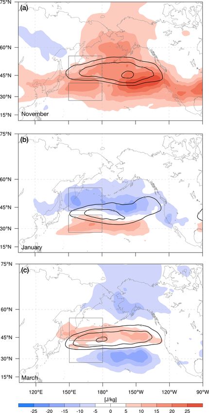
56                                                                  S. Schemm et al.: The North Pacific storm-track suppression

(Schemm and Schneider, 2018). The atypical intraseasonal               reduced because of a reduction in the baroclinic conversion
cycle of baroclinic waves over the North Pacific has triggered         efficiency. Eddies from the northern seeding branch (Chang,
considerable research during the last 2 decades. In the fol-           2005) propagate more equatorward and towards the subtropi-
lowing, we give an overview of the current understanding of            cal jet in midwinter, and during this equatorward propagation
the midwinter suppression.                                             they acquire a stronger than usual poleward tilt with height,
   Factors that have been suggested to contribute to the mid-          which reduces the eddy efficiency because of a weaker align-
winter suppression can be categorized into contributions               ment between the mean baroclinicity and the eddy heat flux
from barotropic, baroclinic, and upstream seeding processes.           (Schemm and Rivière, 2019). Schemm and Rivière (2019)
Among the barotropic contributions are the increase in the             quantified baroclinic conversion for all upper-level eddies
horizontal wind shear near the jet and the deformation acting          and surface cyclones in the western North Pacific. However,
on baroclinic wave packets in a stronger and more narrow               as shown in Sect. 4 of this study, the surface-cyclone tracks
jet stream during midwinter (James, 1987; Nakamura, 1993;              in this sector of the Pacific emerge from three different re-
Harnik and Chang, 2004; Deng and Mak, 2005). However,                  gions: (i) downstream of Kamchatka, (ii) over the Kuroshio
in idealized simulations it was shown that such a barotropic           extension, and (iii) over the East China Sea. So far, it has re-
governing mechanism is not symmetric in time around the                mained unclear whether the suppression affects the cyclones
suppression, and the increase in the horizontal shear lags the         from these genesis regions in a similar way.
onset of the suppression (Novak et al., 2020). With regard                In this study, we investigate midwinter changes in surface-
to upstream seeding processes, a reduction in the amplitude            cyclone life cycles over the western North Pacific accord-
and frequency of upper-level eddies propagating from up-               ing to their genesis region. Surface cyclones are an important
stream into the North Pacific has been suggested to play a             subcategory of the wide distribution of flow features collec-
crucial role in the formation of the midwinter suppression             tively termed “eddies”. Upper-level cyclonic eddies, some
(Penny et al., 2010, 2011, 2013), but this is strongly debated         of them shallow, correspond to troughs. Once a trough in-
because baroclinic growth is decorrelated with the strength            teracts with a surface eddy, they mutually amplify (Hoskins
of upstream seeding (Chang and Guo, 2011, 2012). More-                 et al., 1985, Fig. 21) and propagate poleward in tandem (Gilet
over, a reduced midwinter suppression also occurs in sim-              et al., 2009; Rivière et al., 2012; Oruba et al., 2013). The
ulations with the upstream Asian mountains removed (Park               combined system develops into a mature low-pressure sys-
et al., 2010). The increase in the velocity of eddy propaga-           tem corresponding to a deep cyclonic eddy. With surface-
tion along the baroclinic zone and a reduced lifetime have             cyclone tracks we thus identify particularly strong cyclonic
also been shown to be insufficient to explain the suppres-             eddies that play an essential role in the overall storm-track
sion (Chang, 2001; Nakamura and Sampe, 2002). The reduc-               climatology. Over the North Pacific, we expect to find dif-
tion in the lifetime also occurs over the North Atlantic, which        ferent life-cycle characteristics in midwinter compared to
does not exhibit a suppression in most winters (Schemm and             November and March because in midwinter the cyclones typ-
Schneider, 2018).                                                      ically form on the poleward flank of a strong subtropical jet,
   There is mounting evidence that the shift to a subtropical          whereas in November and March they usually develop on the
jet regime in the western North Pacific is essential for the           equatorward flank of a more poleward-located jet. Schemm
formation of the midwinter suppression. During the shift to a          and Schneider (2018) have already shown that for the en-
subtropical jet regime, the subtropical thermally driven jet in-       tire North Pacific the lifetime of surface cyclones is shortest
creases its strength, shifts equatorward, and extends into the         in midwinter. Here we study in detail all surface cyclones
zonal direction. Idealized studies have shown that the transi-         that affect the region of the midwinter suppression in the
tion to a subtropical jet regime is able to reproduce a realistic      western North Pacific between October and April and quan-
midwinter suppression and thus ruled out the absolute neces-           tify their frequency, lifetime, intensity, baroclinic conversion
sity of zonal asymmetries, such as upstream mountains, for             rates, and other characteristics according to their genesis re-
its formation (Yuval et al., 2018; Novak et al., 2020). The            gion. This approach will serve to address the following ques-
importance of a subtropical jet regime for the formation of a          tions.
storm-track suppression is reinforced by the fact that a mild
suppression is also observed over the North Atlantic in years            – What is the relative contribution of different genesis re-
with strong subtropical jets (Penny et al., 2013; Afargan                  gions to the surface-cyclone frequency in the region af-
and Kaspi, 2017). Chang (2001) and Nakamura and Sampe                      fected by the midwinter suppression?
(2002) already hinted at the potential key role of the subtrop-          – Are there any differences in the character of the surface
ical jet and its meridional displacement relative to the low-              cyclones of different origin between midwinter and the
level zone of highest baroclinicity, but the exact mechanism               shoulder months? For example, how do their number,
that reduces baroclinic growth has remained unclear. Such a                lifetime, and time to maximum intensity vary during the
mechanism was suggested by Schemm and Rivière (2019),                      cold season?
who showed that in the subtropical jet regime the ability of
eddies to extract eddy energy from the mean baroclinicity is

Weather Clim. Dynam., 2, 55–69, 2021                                                        https://doi.org/10.5194/wcd-2-55-2021
S. Schemm et al.: The North Pacific storm-track suppression                                                                    57

    – Is the suppression of the baroclinic conversion during       1955; Orlanski and Katzfey, 1991; Chang, 2001). A detailed
      midwinter equally strong for cyclones of different ori-      derivation of both tendency equations using 10 d high-pass-
      gin?                                                         filtered input data is given in Schemm and Rivière (2019).
                                                                   The baroclinic conversion to eddy energy, which is the sum
   To answer these questions, we use an object-based surface-      of eddy kinetic and eddy available potential energy, is the
cyclone tracking algorithm and evaluate baroclinic conver-         scalar product between the eddy heat flux √1 θ 0 v 0 and the
                                                                                                                   S
sion rates obtained from band-pass-filtered data along indi-                                  ∇θ
vidual cyclone tracks. With this approach, we combine two          background baroclinicity − √  :
                                                                                                 S
complementary perspectives on storm-track dynamics.
   Our study is organized as follows. In Sect. 2 we introduce               1
                                                                   Bconv = − θ 0 v 0 · ∇θ ,                                   (1)
the data and methods used. In Sect. 3 we describe the mid-                  S
winter evolution of eddy kinetic energy (EKE) over the North
                                                                   where v 0 denotes the high-pass-filtered horizontal wind, θ the
Pacific and define specific target regions characterized by an
                                                                   low-pass-filtered potential temperature, and S the static sta-
increase and decrease in EKE during winter, respectively.
                                                                   bility in pressure coordinates S = −h−1 ∂θ    R
                                                                                                               ∂p . The reference
The surface-cyclone tracks and the genesis regions of cy-
                                                                   potential temperature θR is computed from monthly mean
clones that propagate through the target regions are presented
                                                                   data, and h denotes the scale height. Background baroclin-
in Sect. 4. Section 5 presents a detailed analysis of changes
                                                                   icity is defined as the horizontal gradient of the low-pass-
in different life-cycle characteristics. Baroclinic conversion
                                                                   filtered potential temperature divided by the static stability,
along cyclone tracks of different origin is studied in Sect. 6.            ∇θ
We conclude our study in Sect. 7.                                  B = −√      . The background baroclinicity is closely related
                                                                             S
                                                                   to the Eady growth rate (Lindzen and Farrell, 1980). The
                                                                   scalar product that defines the baroclinic conversion can fur-
2     Data and methods                                             ther be decomposed into contributions from the background
                                                                   baroclinicity and the baroclinic conversion efficiency, which
The analysis period is October to April 1979–2018. All di-         is a measure for how efficiently cyclones convert the baro-
agnostics rely on 6-hourly ERA-Interim data that are inter-        clinicity into eddy energy. The baroclinic conversion effi-
polated to a 1◦ grid. ERA-Interim is publicly available for        ciency is connected to the vertical tilt of the growing cy-
download via the ECMWF archive at https://apps.ecmwf.int/          clone and is maximized if the vertical tilt is such that the
datasets/ (last access: January 2021).                             eddy heat flux aligns with the mean baroclinicity – for more
                                                                   details see Schemm and Rivière (2019). We base our anal-
2.1    Surface-cyclone tracks and surface cyclogenesis             ysis on the conversion rates at the 500 hPa level. This is a
                                                                   pragmatic choice because the suppression increases in am-
For the identification and tracking of surface cyclones,           plitude with altitude, while baroclinic conversion is largest
we make use of the algorithm introduced by Wernli and              in the lower troposphere (Schemm and Schneider, 2018). At
Schwierz (2006) and refined by Sprenger et al. (2017). The         the 500 hPa level, the suppression of baroclinic conversion is
detection of surface cyclones is based on a contour search in      a well-marked feature.
the mean sea level pressure (SLP) field at intervals of 0.5 hPa.
To obtain a cyclone mask at each time step, all grid points in-
side the outermost closed contour, which must not exceed           3   EKE of the North Pacific storm track in midwinter
7500 km in length, are labeled with 1 and all others with 0.
The obtained binary cyclone fields are used to compute cy-         This section recapitulates the seasonal cycle and transition
clone frequencies. Cyclone centers are defined as the grid         of the North Pacific storm track as seen in EKE at 500 hPa.
point with minimum SLP inside the outermost closed con-            In November, EKE increases relative to October across the
tour. The cyclone centers are tracked using 6-hourly cyclone       entire North Pacific (red shading in Fig. 1a), with the max-
center positions, and a track is accepted if it exists for a pe-   imum increase over the eastern North Pacific near 150◦ W.
riod of at least 1 d. The first time step along each track is      In January, EKE is reduced compared to December in an
defined as the genesis time step, and the SLP minimum de-          elongated band across the Pacific north of ∼ 43◦ (blue shad-
fines the genesis location. The algorithm contributed to the       ing in Fig. 1b). Equatorward of this latitude, however, EKE
cyclone identification and tracking intercomparison project        increases (red shading in Fig. 1b). This dipole pattern in
of Neu et al. (2013).                                              EKE tendency results from the equatorward shift of the
                                                                   North Pacific jet during midwinter. Absolute values of EKE
2.2    Baroclinicity and baroclinic conversion                     (black contours in Fig. 1b) are reduced compared to those
                                                                   in November, which is due to the stronger EKE reduction
The background baroclinicity and the corresponding baro-           poleward of ∼ 43◦ N compared to the simultaneous increase
clinic conversion are defined based on tendency equations          equatorward (see Fig. 1 in Schemm and Schneider, 2018, for
for eddy kinetic and available potential energy (Lorenz,           a more detailed discussion of month-to-month EKE varia-

https://doi.org/10.5194/wcd-2-55-2021                                                   Weather Clim. Dynam., 2, 55–69, 2021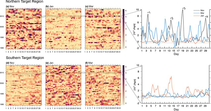
58                                                                    S. Schemm et al.: The North Pacific storm-track suppression

Table 1. Total number (first column) of surface cyclones in the
northern target region and number of cyclones per day in paren-
theses (1980–2018). Fraction and number (in parentheses) of (sec-
ond column) Kamchatka, (third column) Kuroshio, and (fourth col-
umn) East China Sea cyclones. The northern target region is shown
in Fig. 1. For the genesis locations, the following definitions are
used (see also Fig. 2). Kuroshio cyclones: south of 45◦ N and east
of 135◦ E. East China Sea cyclones: south of 45◦ N and west of
135◦ E. Kamchatka cyclones: north of 45◦ N.

                Cyclones in    Kamchatka    Kuroshio          East
               target region                             China Sea
    November    507 (0.43)     45 % (229)   41 % (207)    14 % (71)
    January     516 (0.43)     40 % (206)   46 % (236)    14 % (74)
    March       527 (0.44)     39 % (208)   39 % (204)   22 % (115)

tions). From February to March, EKE increases again in a
meridionally confined band between ∼ 40◦ and 50◦ N and
decreases equatorward of ∼ 40◦ . Based on theses patterns
of intraseasonal changes in EKE, we select in the following
surface cyclones that propagate through one of the regions
with a midwinter (December to January) EKE decline or in-
crease, respectively. The two target regions are indicated as
gray boxes in Fig. 1 and are located at the entrance of the
storm track (EKE maximum). One of our aims is to assess if
and how the EKE tendency dipole seen in Fig. 1b is linked
to characteristics of the surface-cyclone tracks. We focus in
particular on cyclones that propagate through the northern
target region, which exhibits a decline in EKE during mid-
winter and is therefore essential for understanding the mid-
winter suppression phenomenon.

4     Surface-cyclone view on the North Pacific storm
      track in midwinter

4.1    Surface cyclogenesis

Consideration is first given to cyclogenesis associated with
surface-cyclone tracks that propagate through the northern
target region, i.e., the region where EKE decreases during               Figure 1. Mean EKE at the 500 hPa level (black contours at 85,
midwinter (Fig. 1b). To this end, we extract all tracks for              95, and 105 J kg−1 ) and corresponding change relative to the corre-
which the cyclone center is inside the target region for at least        sponding previous month (color shading) for (a) November, (b) Jan-
one time step. In November, these surface cyclones originate             uary, and (c) March. Additionally shown are two target regions
from two preferred regions (Fig. 2a). The first region is lo-            (gray boxes) that are used for the detailed diagnostics of surface-
cated over the Kuroshio extension (near 35◦ N) and the sec-              cyclone tracks throughout this study.
ond region downstream of the Kamchatka Peninsula (near
53◦ N). This pattern and the number of events are fairly sim-
ilar in January (Fig. 2c). In March (Fig. 2e), a third cycloge-
                                                                            The southern target region, i.e., the region where EKE in-
nesis region emerges southwest of Japan over the East China
                                                                         creases during midwinter (Fig. 1b), is fed exclusively by sur-
Sea (near 30◦ N), while the other two cyclogenesis regions
                                                                         face cyclones with genesis over the Kuroshio extension dur-
retain fairly similar frequencies. For cyclones propagating
                                                                         ing November (Fig. 2b). In January, a second but weaker cy-
through the target region of the midwinter suppression, there
                                                                         clogenesis region emerges southwest of Japan over the East
is no signal of a suppression in the genesis and therefore the
                                                                         China Sea. In March (Fig. 2f), the two genesis regions ex-
number of these cyclones (Table 1).
                                                                         hibit similar cyclogenesis frequencies and contribute equally

Weather Clim. Dynam., 2, 55–69, 2021                                                           https://doi.org/10.5194/wcd-2-55-2021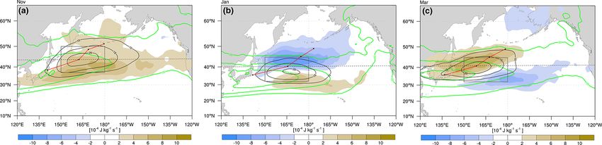
S. Schemm et al.: The North Pacific storm-track suppression                                                                             59

Figure 2. Cyclogenesis frequency (color shading; %) for surface-cyclone tracks that propagate through the northern (a, c, e) and south-
ern (b, d, f) target regions (shown as a gray box) for (a, b) November, (c, d) January, and (e, f) March. Additionally shown are EKE (black
contours; 85, 95, and 105 J kg−1 ) and baroclinicity (green contours; 25 to 45 × 10−6 s−1 by steps of 5 × 10⁻⁶ s−1 ) at the 500 hPa level.

to the cyclone tracks in the southern target region. Notably,           preferred regions of surface cyclogenesis (Fig. 2) by means
for this region there is also no midwinter suppression in the           of lagged 300 hPa geopotential anomalies. We find that Kam-
cyclone frequency. This result is in agreement with the find-           chatka and Kuroshio cyclogenesis is triggered by waves en-
ings of Schemm and Schneider (2018) that the suppression                tering the North Pacific from the northern seeding branch
is connected to a reduction in the cyclones’ intensity rather           over Siberia (Fig. S1 in the Supplement), which in January
than frequency.                                                         have a more equatorward propagation direction, in agree-
   Surface cyclones over the North Pacific are known to be              ment with Schemm and Rivière (2019). After surface cy-
triggered by two upper-level seeding branches: a northern               clogenesis, the upper-level wave packet retains its overall
branch over Siberia and a southern branch along the sub-                more zonal orientation (Fig. S1). Cyclogenesis over the East
tropical jet across southern Asia (Chang, 2005). We briefly             China Sea is associated with the southern seeding branch
report on the upper-level seeding associated with the three             and an upper-level trough downstream of the genesis loca-

https://doi.org/10.5194/wcd-2-55-2021                                                        Weather Clim. Dynam., 2, 55–69, 2021
60                                                                 S. Schemm et al.: The North Pacific storm-track suppression

tion (not shown). This behavior was already recognized by             Table 2. Mean lifetime (h) of surface cyclones passing through the
Chang (2005), who noted that “cyclogenesis for these cases            northern target region according to their genesis regions.
is probably not triggered by the (upper-level) wave packet”
(Chang, 2005, p. 1998). The genesis of these cyclones seems                             Kamchatka      Kuroshio    East China Sea
to be connected to a bottom-up development, as is the case                 November          77           98             117
for diabatic Rossby waves (e.g., Boettcher and Wernli, 2013).              January           62           86             132
                                                                           March             70           91             172
4.2    Relative surface-cyclone frequencies

In the previous section, we showed that surface cyclogene-            Table 3. Mean time to maximum deepening since genesis (h) of
sis downstream of Kamchatka, over the Kuroshio extension,             cyclones passing through the northern target region according to
and in late winter over the East China Sea contributes to the         their genesis regions.
surface-cyclone tracks in the northern target region, where
EKE exhibits a midwinter suppression. To study the relative                             Kamchatka      Kuroshio    East China Sea
importance of the tracks generated in the different genesis re-            November          35           29             43
gions for the total cyclone frequency in the target region and             January           26           21             39
elsewhere, we group the cyclone tracks into two categories.                March             31           23             42
The first contains tracks with genesis over the Kuroshio ex-
tension or the East China Sea, which enter the target region
from the south. The second category contains tracks with              gion (gray box in Fig. 1), where EKE decreases during mid-
genesis near Kamchatka that propagate through the target re-          winter.
gion. Next, we compute cyclone frequency fields for the two              The lifetime from genesis to lysis of Kamchatka and
categories at every grid point and divide them by the total cy-       Kuroshio cyclones is shortest in January and larger in
clone frequency field obtained from all cyclone tracks. The           November and March (Table 2). This is what one might
obtained relative contributions are shown for November, Jan-          expect from the strong midwinter jet and the fact that
uary, and March in Fig. 3. During all months, Kamchatka cy-           over the North Atlantic the shortest cyclone lifetimes are
clones contribute up to 40 %–50 % along the poleward side of          also observed during midwinter (Schemm and Schneider,
the target region and only 10 %–20 % along the equatorward            2018). However, it could also result from the fact that these
side. The relative contribution of cyclone tracks entering the        poleward-propagating cyclones leave the more equatorward-
target region from the south is 80 %–90 % along the equator-          located baroclinic zone earlier. Finally, the lifetime of East
ward side of the box and decreases towards higher latitudes to        China Sea cyclones increases from November to March.
50 %–60 % along the poleward side of the target region. The              The time to maximum deepening since cyclogenesis is
relative contributions indicate the tendency of the selected          shortest during midwinter, independent of the cyclogenesis
cyclone tracks to propagate poleward. For example, less than          region (Table 3). Maximum deepening is measured in Berg-
20 % of the cyclone tracks propagated from the Kuroshio re-           eron, which is the 24 h change in sea level pressure along
gion across the Pacific and into the Gulf of Alaska. Figure 3         a cyclone track normalized to 60◦ N (Sanders and Gyakum,
further corroborates the fact that the midwinter suppression          1980). Because the cyclogenesis regions exhibit almost no
is related to a change in the characteristics of these cyclones       variations in terms of their exact location (Fig. 2), the re-
and not in their frequencies. Also, we cannot focus on ei-            duced time to maximum deepening for Kuroshio and East
ther Kuroshio or Kamchatka cyclones only because they both            China Sea cyclones could result from the more equatorward
substantially contribute to the total cyclone frequency in the        location of the zone of highest baroclinicity. These poleward-
target region. In the following, we study statistics of cyclone       propagating systems eventually leave the baroclinic zone ear-
characteristics for the different genesis regions in greater de-      lier in midwinter, which explains the reduced lifetime and
tail.                                                                 the shorter time to maximum deepening. For Kuroshio and
                                                                      East China Sea cyclones, the mean latitude where maxi-
                                                                      mum deepening occurs is therefore also shifted by around 2◦
5     Detailed characteristics of surface-cyclone life cycle          equatorward in January compared to November (not shown),
                                                                      which is in agreement with the earlier deepening.
In the previous section, we showed that the northwestern                 With regard to the minimum sea level pressure as a mea-
Pacific surface storm track is fed by three preferred cyclo-          sure of the storm intensity, Kamchatka cyclones become less
genesis regions: (i) the East China Sea, (ii) Kuroshio, and           intense from November to March (Table 4). East China Sea
(iii) Kamchatka; neither of the three exhibits a midwin-              cyclones are most intense during midwinter, but they con-
ter suppression in terms of cyclogenesis frequency (Fig. 2).          tribute only 22 % to the total cyclone number (Table 1).
Next, we investigate several life-cycle characteristics. As in        Kuroshio cyclones are also most intense in January, but the
the previous sections, our focus is on the northern target re-        change in minimum SLP between November and January is

Weather Clim. Dynam., 2, 55–69, 2021                                                        https://doi.org/10.5194/wcd-2-55-2021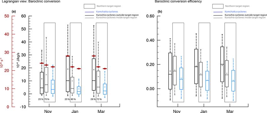
S. Schemm et al.: The North Pacific storm-track suppression 61
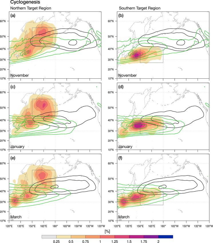
Figure 3. Relative contributions (color shading; %) of (a, c, e) Kamchatka cyclones and (b, d, f) Kuroshio combined with East China Sea
cyclones to the total surface-cyclone frequency in the northern target region (gray box). The contours show the change in EKE relative to
the corresponding previous month (solid lines are for positive values and dashed lines for negative values; −20 to 20 J kg−1 by steps of
5 J kg−1 ).
small. The equatorward movement of the baroclinic zone in with the increase in the background baroclinicity. Kuroshio
midwinter seems to be beneficial for the intensification of cyclones thus appear to deepen rapidly in a short time pe-
East China Sea cyclones in January. Kamchatka cyclones, riod (Table 3), in agreement with the midwinter peak in
however, become less intense, a result that can, at least qual- baroclinicity, but after reaching their strongest intensity they
itatively, be expected from the equatorward retreat of the also decay rapidly, as indicated by the shortest lifetime dur-
baroclinic zone. For Kuroshio cyclones the situation is com- ing midwinter (Table 2). This suggests that for Kuroshio cy-
plex. While there is a weak reduction in the minimum SLP clones the peak in baroclinic conversion occurs earlier dur-
from November to January, the fraction of life cycles that ing their life cycle and the short deepening is also more in-
satisfy the Sanders and Gyakum (1980) criterion for explo- tense, but thereafter they move out of the zone of high baro-
sive deepening, known as “bomb cyclogenesis”1 , is reduced clinicity relatively soon, resulting in less intense cyclones at
in midwinter. In contrast, for the East China Sea cyclones higher latitudes. This could also explain the dipole pattern
the bomb fraction peaks in January, which is in agreement in EKE shown in Fig. 1b because in January approximately
50 % of all cyclone tracks that propagate through the north-
1 A change in SLP larger than 24 hPa within 24 h normalized to ern target region also propagate through the southern target
60◦ N (Sanders and Gyakum, 1980). region. Thus, to better understand the intensification, in the
https://doi.org/10.5194/wcd-2-55-2021 Weather Clim. Dynam., 2, 55–69, 202162 S. Schemm et al.: The North Pacific storm-track suppression
Table 4. Mean minimum sea level pressure of surface cyclones more, the difference between January and March is less clear
passing through the northern target region according to genesis re- in the southern target region.
gions and, in parenthesis, the fraction of cyclones satisfying the The above findings suggest that the characteristics of the
criterion for “bomb cyclogenesis” (deepening larger than 24 hPa synoptic systems that propagate through the two target re-
within 24 h normalized to 60◦ N.) gions shown in Fig. 1 clearly differ between the three months.
In January, the associated baroclinic conversion is lower than
Kamchatka Kuroshio East China Sea
in November and March in the northern target region and
November 979.4 (21 %) 975.8 (49 %) 975.7 (63 %) vice versa for the southern region. There are several possible
January 982.9 (7 %) 973.6 (42 %) 967.2 (76 %) explanations for this behavior. For instance, (i) in midwinter,
March 987.3 (7 %) 979.0 (43 %) 971.4 (65 %) baroclinic conversion is reduced along the entire life cycle of
cyclones in the northern region, or (ii) the life cycles of those
cyclones that propagate through both target regions, which
are about ∼ 50 % of all cyclones that enter the northern target
next section we investigate baroclinic conversion first over
region from the south, have an earlier baroclinic conversion
the two target regions from an Eulerian viewpoint and after-
peak (in the southern target region) and reduced baroclinic
ward along the different tracks using feature-based cyclone
conversion later in the northern target region. As we show
tracking.
below, the first scenario applies to Kamchatka cyclones and
the second one to Kuroshio cyclones. But first, we explore
how baroclinic conversion changes during days when a cy-
6 Baroclinic conversion and its relationship with clone propagates through the northern target region.
surface-cyclone tracks
6.2 Baroclinic conversion in the northern target region
6.1 Baroclinic conversion over target regions (Eulerian associated with surface cyclones
perspective)
In order to quantify the contribution of surface cyclones
EKE has a baroclinic and barotropic source, and both are to the climatological monthly mean baroclinic conversion
known to be affected by a midwinter suppression (Schemm in the northern region, we split all days into cyclone and
and Schneider, 2018). In general, however, the dominant non-cyclone days using the surface-cyclone tracks. Thereby,
source of EKE is baroclinic conversion. In the following, we we essentially separate deep eddies that extend throughout
first diagnose variations in baroclinic conversion and its link the troposphere, like mature cyclones, and shallow diabat-
to surface cyclones in the northern and southern target re- ically maintained low-level cyclonic eddies, like diabatic
gions on synoptic timescales. The daily mean values of baro- Rossby waves, from upper-level shallow eddies, like troughs
clinic conversion, averaged over the northern and southern or ridges. Anticyclonic eddies are also excluded. Technically,
target regions (see Fig. 1), are shown in Fig. 4 for Novem- a surface-cyclone track may propagate outside the northern
ber, January, and March. Baroclinic conversion often peaks target region but nevertheless affect the baroclinic conver-
at regular intervals of 6–10 d (see the zoom-in for Novem- sion inside the target region. We therefore define a cyclone
ber 2009 as well as January and March 2010 in the right day as a time step when 25 % of the northern target region
panels of Fig. 4). These baroclinic conversion bursts result is covered by a cyclone mask (see Sect. 2 for details). This
mostly, but not exclusively, from the propagation of deep results in about 50 % cyclone and 50 % non-cyclone days.
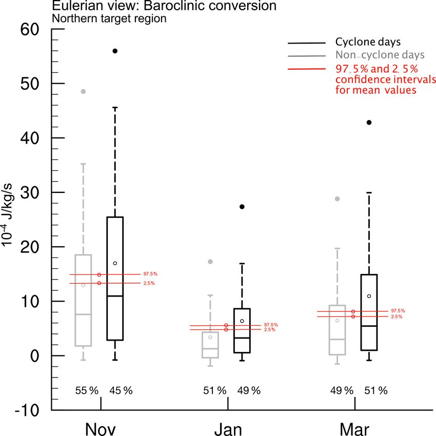
synoptic systems through the target region. In the northern Baroclinic conversion is, as expected, larger during cy-
target region in November 2009 (black contours in the top clone days compared to non-cyclone days (Fig. 5), but baro-
right panel of Fig. 4), the first and third bursts (labeled 1 clinic conversion is not zero during non-cyclone days. Only
and 3 in Fig. 4) are associated with Kuroshio cyclones, while in January is the median of the baroclinic conversion distri-
the fourth one is associated with a Kamchatka cyclone that bution near zero for non-cyclone days. The fact that baro-
propagates north of the target region but still affects a broader clinic conversion is not zero during non-cyclone days can
region around it. The second burst (13–15 November) is not be explained by baroclinic conversion related to an upper-
associated with a surface cyclone but with a jet streak devel- level trough propagating over the northern target region that
opment at the edge of an upper-level trough. In November is not accompanied by a surface cyclone, as is the case for the
and March (black and blue contours in the top right panel of second burst in Fig. 4 (upper right panel). As clearly shown
Fig. 4), the amplitude of the bursts exceeds those in January in Fig. 5, the midwinter suppression affects baroclinic con-
by a factor of 2–3 (orange contour). The opposite is found version during cyclone and non-cyclone days. Yet, the two
in the southern target region, where the baroclinic conver- distributions differ significantly from each other, in partic-
sion bursts in January exceed those in November and March. ular in January during midwinter suppression. To test this
However, the monthly differences in the southern target re- statistically, we compute 10 000 distributions, each of which
gion are smaller than in the northern target region. Further- consists of randomly selected cyclone and non-cyclone days
Weather Clim. Dynam., 2, 55–69, 2021 https://doi.org/10.5194/wcd-2-55-2021S. Schemm et al.: The North Pacific storm-track suppression 63 Figure 4. Baroclinic conversion at 500 hPa (10−3 J kg−1 s−1 ) averaged over the (a–c) northern and (d–f) southern target regions shown in Fig. 1 for (a, d) November, (b, e) January, and (c, f) March for the period 1979–2018. Attached on the right side is a zoomed-in image of the individual time series of daily mean values for November (2009), January (2010), and March (2010). with replacement. Each randomized distribution is of equal those cyclone tracks that enter the northern target region from size as the original cyclone day distribution. For each ran- the south and compare the baroclinic conversion along these domized distribution, we compute the mean baroclinic con- tracks before and after entrance. version, and from the 10 000 mean values we compute per- centiles 97.5 and 2.5, which are shown as red confidence in- 6.3 Baroclinic conversion along cyclone tracks outside tervals in Fig. 5. The mean baroclinic conversion values of and inside the northern target region (Lagrangian the cyclone (non-cyclone) day distribution is above (below) perspective) the 97.5 % (2.5 %) confidence intervals in each month. We therefore conclude that the two distributions significantly dif- Cyclones that feed the northern target region are Kamchatka fer from each other and from a randomized selection. Based cyclones, with genesis inside the target region, and Kuroshio on Fig. 5, we conclude that baroclinic conversion in the target and East China Sea cyclones, which enter the target region region is reduced in midwinter both during cyclone days and from the south. We therefore group all time steps along non-cyclone days. However, since the baroclinic conversion Kuroshio and East China Sea cyclone tracks into two periods, during cyclone days is higher than during non-cyclone days, before and after entering the northern target region. The idea the cyclone days contribute in absolute terms more to the to- is to see whether the maximum baroclinic conversion occurs tal baroclinic conversion in the Pacific storm track. Never- earlier during the life cycle in January, as suggested in Sect. 5 theless, the relative contribution to the suppression is fairly and based on Table 3, and therefore outside the northern tar- similar. The average baroclinic conversion on a cyclone day get region. In the following, we discuss box-and-whisker dia- is reduced from 17 to 6×10⁻⁴ J kg s−1 and on a non-cyclone grams of baroclinic conversion, the background baroclinicity day from 13 to 3 × 10⁻⁴ J kg s−1 , and the number of days in (Fig. 6a), and the baroclinic conversion efficiency (Fig. 6b) each category is close to 50 % (Fig. 5). The separation into separately for cyclones that enter the target region from the cyclone days and non-cyclone days is not clear-cut. We de- south (Kuroshio and East China Sea cyclones) for time steps fined non-cyclone days as those days during which the tar- before and after entering the target region and for Kamchatka get region is less than 25 % covered with a cyclone mask. cyclones, which reside inside the target region. For all cy- Baroclinic conversion on non-cyclone days might thus still clones, baroclinic conversion and its efficiency are averaged be associated with surface cyclones in close proximity to the within a 1000 km radius around the cyclone center. target region. In a next step, we investigate in more detail https://doi.org/10.5194/wcd-2-55-2021 Weather Clim. Dynam., 2, 55–69, 2021
64                                                                         S. Schemm et al.: The North Pacific storm-track suppression

                                                                              hence out of the zone of high baroclinicity as originally hy-
                                                                              pothesized by Nakamura (1992). On their way poleward,
                                                                              they also become less efficient in converting the mean baro-
                                                                              clinicity (Fig. 6b). The reduction of baroclinic conversion in
                                                                              the northern target region in January occurs despite the fact
                                                                              that the mean baroclinicity along the tracks of Kuroshio cy-
                                                                              clones is only marginally reduced compared to other months
                                                                              (horizontal red bars on top of the gray box-and-whisker dia-
                                                                              grams in Fig. 6). Equatorward of the target region, the baro-
                                                                              clinic conversion efficiency in January is higher compared
                                                                              to November, but once Kuroshio cyclones have entered the
                                                                              target region the conversion efficiency declines and is lower
                                                                              in January. In November, the mean efficiency even increases
                                                                              when Kuroshio cyclones enter the northern target region. The
                                                                              conversion budget discussed in Schemm and Rivière (2019)
                                                                              showed that the reduced baroclinic conversion in this region
                                                                              indeed results from a reduction in both the mean baroclin-
                                                                              icity and the conversion efficiency, with the conversion effi-
                                                                              ciency making the larger contribution to the reduction. Over-
                                                                              all, the results presented here indicate that Kuroshio cyclones
                                                                              in January deepen rapidly equatorward of the target region
Figure 5. Box-and-whisker diagram of baroclinic conversion at                 and their growth is even stronger compared with November
500 hPa (10−4 J kg−1 s−1 ) averaged over the northern target re-
                                                                              and March, but on their way poleward their conversion effi-
gion (gray box in Fig. 1) for days (black) with and (gray) with-
out a surface cyclone affecting the target region (referred to as cy-
                                                                              ciency decreases, in agreement with the dipole anomaly seen
clone and non-cyclone days). Whiskers span between the 10th and               in Fig. 4 in Schemm and Rivière (2019). The stronger growth
90th percentiles and the box spans the 25th to 75th percentile range.         in January equatorward of the target region appears to accel-
Filled dots indicate the 95th percentile. Open circles indicate the           erate the life cycle, and the cyclones seem to reach a stage
mean value and horizontal lines the median value. The 2.5 % and               when they become less efficient at converting the mean baro-
97.5 % confidence intervals of a statistical test (see text for details)      clinicity into eddy energy earlier during the life cycle.
are shown in red. Percentage values at the bottom indicate the frac-             For Kamchatka cyclones, baroclinic conversion is reduced
tion of days in each sample.                                                  in midwinter compared to the shoulder months (blue boxes
                                                                              in Fig. 6), in agreement with the reduced baroclinicity and
                                                                              reduced efficiency (Fig. 6b). The re-intensification of Kam-
   Before entering the northern target region from the south,                 chatka cyclones during March occurs despite no notable
baroclinic conversion along cyclone tracks is larger in Jan-                  change in the mean baroclinicity (horizontal red bars on top
uary than in November and March (black boxes in Fig. 6).                      of the blue box-and-whisker diagrams in Fig. 6), a finding
The distribution of baroclinic conversion outside the target                  that again points towards an increase in the baroclinic con-
region exhibits a seasonal cycle that is qualitatively in agree-              version efficiency as an important moderating process. Kam-
ment with the seasonal cycle of the mean baroclinicity equa-                  chatka cyclones contribute with 40 % to the storm track over
torward of the target region. The difference between January                  the northern target region, and their weakening is therefore
and March is small, which is a result of the increasing in-                   an important contribution to the suppression.
fluence of East China Sea cyclone tracks towards late winter                     In summary, maximum baroclinic conversion along the
and early spring. East China Sea cyclones deepen on average                   surface-cyclone tracks with genesis over the Kuroshio exten-
more rapidly than Kuroshio cyclones (Table 4), and they are                   sion is climatologically largest in January but occurs equa-
particularly frequent in March (Fig. 2 and Table 1).                          torward of the northern target region and therefore earlier
   After entering the northern target region, baroclinic con-                 during the cyclone life cycle. The larger conversion is thus
version associated with Kuroshio and East China Sea cy-                       in agreement with an overall higher mean baroclinicity over
clones is reduced in January compared to November and                         the North Pacific, but the equatorward shift of the strength-
March, which reflects the midwinter suppression (gray boxes                   ened baroclinic zone causes earlier intensification because
in Fig. 6). Kuroshio cyclones spend most of their life cycle                  the zone shifts towards the preferred region of Kuroshio cy-
in the northern target region (the percentage of time steps                   clogenesis. Kuroshio cyclones not only leave the zone of
in each category is shown below each box in Fig. 6). In                       highest baroclinicity faster in midwinter, but on their way
January, the fraction of time steps outside the northern tar-                 poleward they also become less efficient at converting the
get region is lower than in November and March, suggest-                      mean baroclinicity into eddy energy. For Kamchatka cy-
ing that in January cyclones propagate poleward faster and                    clones, the change throughout the cold season is in fairly

Weather Clim. Dynam., 2, 55–69, 2021                                                               https://doi.org/10.5194/wcd-2-55-2021
S. Schemm et al.: The North Pacific storm-track suppression 65
Figure 6. Box-and-whisker diagram for (a) baroclinic conversion at 500 hPa (10−4 J kg−1 s−1 ) averaged within a radius of 1000 km around
the surface-cyclone centers of Kuroshio and East China Sea cyclones before (black) and after (gray) entering the northern target region, as
well as for Kamchatka cyclones (blue). Additionally shown are the mean background baroclinicity along the tracks (red horizontal lines) and
the percentage of time steps before and after entering the target region. (b) Similar to (a) but for the baroclinic conversion efficiency.
good agreement with what must be expected from a reduc- baroclinic conversion in all months (black contours in Fig. 7).
tion in the background baroclinicity during midwinter and This underlines the fact that the selected tracks play an im-
an increase in early spring. portant role in shaping the monthly mean baroclinic conver-
sion. The mean location of the maximum deepening is lo-
6.4 Baroclinic conversion along cyclone tracks in a cated farthest equatorward during January (Fig. 7b). We split
target region that shifts with the maximum these tracks into time steps before and after the cyclones have
monthly mean baroclinic conversion crossed the latitude of the maximum deepening (dashed lines
in Fig. 7) and compute box-and-whisker plots of the corre-
In the previous sections, attention was given to baroclinic sponding baroclinic conversion rates. The results show that
conversion in a target region that is centered on the location in every month, baroclinic conversion rates are higher be-
of the maximum reduction in EKE during midwinter. In this fore the maximum deepening is reached. When comparing
section, we explore baroclinic conversion associated with cy- the three months, we find that baroclinic conversion is high-
clone tracks that propagate through a target region that shifts est during January (black boxes in Fig. 8). An important fea-
with the location of the maximum monthly mean baroclinic ture of the suppression is the drop in baroclinic conversion in
conversion (black target box in Fig. 7). The maximum is lo- January after maximum deepening (difference between the
cated over the western North Pacific throughout the winter black and gray boxes in Fig. 8), which is larger in January
and shifts equatorward in January. The target box, which has compared to November and March. Consequently, we arrive
the same latitudinal and longitudinal range in each month, at similar conclusions as in the previous section. During Jan-
is shifted latitudinally only. Baroclinic conversion decreases uary, the cyclones benefit from the increased baroclinicity
north of approximately 41◦ N in January and increases south early during the life cycle, but due to the equatorward shift
of it (blue shading in Fig. 7a). Next, in line with our previous of the baroclinic zone the maximum in baroclinic conver-
analysis, we identify all surface-cyclone tracks that propa- sion occurs at lower latitudes (second black dot along the red
gate into this target region from upstream. Figure 7 shows mean track in Fig. 7). The cyclones leave the baroclinic zone
the mean position of the selected tracks (red lines in Fig. 7). early on their way poleward, which can be deduced from
The black dots along this mean track indicate the mean lo- the mean cyclone tracks in Fig. 7, and baroclinic conversion
cation of cyclogenesis, the location of maximum deepening is reduced to levels below that found during November and
(defined as the largest 6-hourly reduction in mean SLP), the March after the cyclones cross the latitude where maximum
location of maximum intensity (defined as the minimum in deepening is observed.
SLP), and the mean location of cyclolysis. The first result is
that the mean location at maximum deepening (second black
dot along the red line) is either exactly at (November, March)
or very close to the location of the maximum monthly mean
https://doi.org/10.5194/wcd-2-55-2021 Weather Clim. Dynam., 2, 55–69, 202166 S. Schemm et al.: The North Pacific storm-track suppression
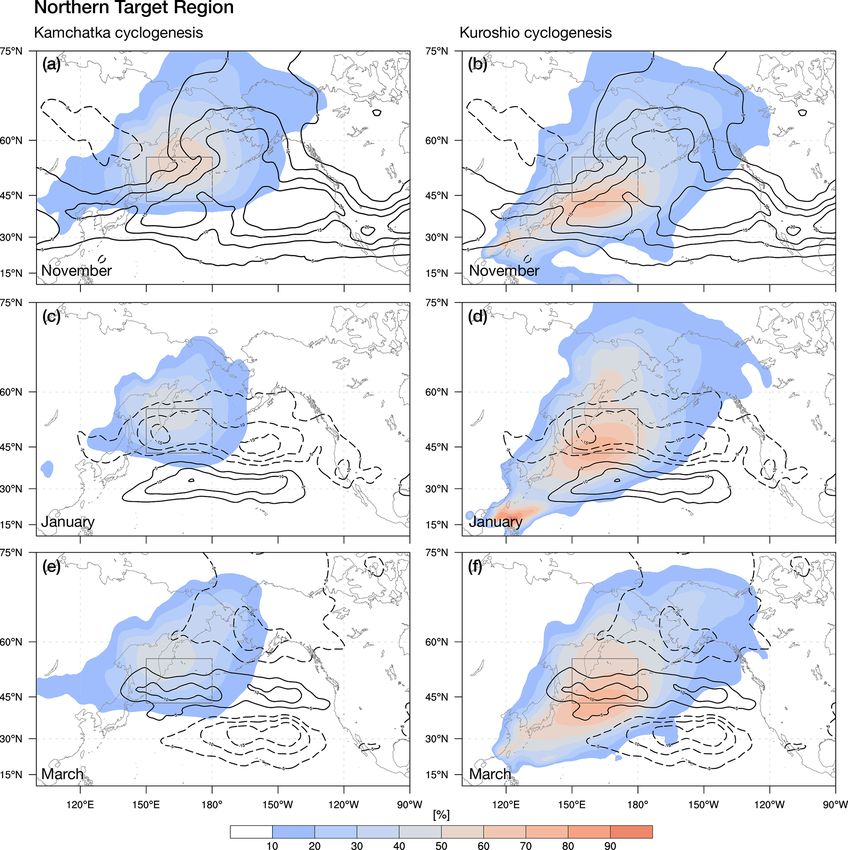
Figure 7. Monthly mean baroclinic conversion at 500 hPa (black contours, 10−4 J kg−1 s−1 ), its change relative to the previous month (color
shading), and a target region (black box) that shifts with the maximum in the mean baroclinic conversion for (a) November (150–180◦ E,
37–50◦ N), (b) January (150–180◦ E, 32–45◦ N), and (c) March (150–180◦ E, 33–46◦ N). The red line indicates the mean location of cyclone
tracks that propagate into the target region from upstream. The black dots along the mean track indicate the mean location of cyclogenesis, the
location of maximum deepening (6-hourly SLP change), the location of maximum intensity (minimum SLP), and the location of cyclolysis.
Additionally shown is the monthly mean baroclinicity (green contours; 25 to 45 × 10−6 s−1 by steps of 5 × 10⁻⁶ s−1 ). The latitude of the
maximum deepening is indicated by a black dashed contour.
7 Conclusions
This study presents a systematic analysis of the character-
istics of cyclone life cycles over the North Pacific with a
particular focus on surface cyclones that propagate through
the western North Pacific, where EKE decreases during mid-
winter (referred to as the northern target region shown in
Fig. 1), and on surface cyclones that propagate through a tar-
get region that shifts latitudinally with the maximum in baro-
clinic conversion (Fig. 7). The goal of this study is to enrich
the existing literature on the midwinter suppression of the
North Pacific storm track with a systematic surface-cyclone
life-cycle perspective to understand how cyclone life cycles
change during midwinter in the western North Pacific.
The surface-cyclone tracks feeding the storm track in the
western North Pacific originate from three preferred regions: Figure 8. Box-and-whisker diagram for baroclinic conversion at
(i) downstream of Kamchatka, (ii) over the Kuroshio exten- 500 hPa (10−4 J kg−1 s−1 ) averaged within a radius of 1000 km
sion, and (iii) over the East China Sea (Fig. 2). Kuroshio around the surface-cyclone centers that enter the target region in
Fig. 7 from upstream before (black) and after (gray) passing the
and Kamchatka cyclones dominate the total cyclone num-
latitude of maximum deepening (black dashed line in Fig. 7).
ber over the western North Pacific throughout the cold sea-
son, while East China Sea cyclones become relevant during
spring. Kamchatka and Kuroshio cyclones are preferentially
triggered by upper-level waves entering the Pacific through since genesis is reduced, and they become less intense.
the northern seeding branch, while East China Sea cyclones They contribute about 40 % to the total cyclone number
are low-level features at genesis (Chang, 2005). The analyzed in winter over the western North Pacific, where EKE is
tracks have their lysis mostly poleward of their genesis loca- suppressed. The weakening of Kamchatka cyclones is
tion in the mid-Pacific. Cyclones in the eastern North Pacific thus a crucial contribution to the suppression. Interest-
thus require further analysis. ingly, despite the reduced baroclinicity in January, the
Our key findings can be summarized as follows. The equa- number of Kamchatka cyclones is not reduced in mid-
torward movement of the baroclinic zone in midwinter af- winter. Kamchatka cyclones do not re-intensify during
fects the life cycles of cyclones from all three genesis re- March, and thus they do not benefit from the poleward
gions, but in a different way. movement of the baroclinic zone in spring.
– Kamchatka cyclones develop in midwinter in a region – East China Sea cyclones benefit from the equatorward
of reduced baroclinicity. Compared to November, their movement of the baroclinic zone in midwinter. Com-
lifetime decreases, the time to maximum deepening pared to November, they become more intense, the frac-
Weather Clim. Dynam., 2, 55–69, 2021 https://doi.org/10.5194/wcd-2-55-2021S. Schemm et al.: The North Pacific storm-track suppression 67
tion of explosively deepening cyclones increases, and more frequent in midwinter because the lifetime of all sys-
their lifetime increases. They become weaker in March, tems is reduced in January. Baroclinic conversion also occurs
but the fraction of explosively deepening life cycles in the absence of surface cyclones, for example through the
remains higher than for Kuroshio and Kamchatka cy- propagation of an upper-level trough, like the second baro-
clones. In addition, their lifetime is longer in March clinic conversion peak in Fig. 4. Baroclinic conversion dur-
compared to January. In March, East China Sea cy- ing non-cyclone days is also affected by the midwinter sup-
clones contribute nearly 22 % to the total cyclone num- pression, and this reduction is not explained by our study.
ber over the northwestern Pacific, while in fall and win- Our study is focused on the western North Pacific, where cli-
ter their contribution is approximately 15 %. Thus, they matological mean baroclinicity is highest and the reduction
seem to play a role in the re-intensification of the storm in baroclinic conversion and EKE is thus most surprising.
track during spring. Cyclone tracks that feed the eastern North Pacific are gener-
ated over the central eastern Pacific (Hoskins and Hodges,
– The changes in the life cycles of Kuroshio cyclones are
2002; Wernli and Schwierz, 2006) where climatologically
the most complex, but understanding these changes is
baroclinicity is much lower compared with the western Pa-
crucial because Kuroshio cyclones contribute the most
cific. Cyclone tracks over the eastern North Pacific not sur-
to the total cyclone number in the northern target re-
prisingly have a large fraction of secondary cyclones (Fig. 5b
gion in midwinter (45 %). Compared to the shoulder
in Schemm et al., 2018). Mechanisms responsible for the
months, in January the lifetime of Kuroshio cyclones
suppression in the eastern North Pacific thus require further
and the time to maximum deepening are shortest. The
analysis.
fraction of cyclones satisfying the “bomb cyclogenesis”
criterion (Sanders and Gyakum, 1980) first decreases
from November to January but then remains at simi- Data availability. ERA-Interim is publicly available for download
lar levels until March. However, the highest values in via the ECMWF archive at https://apps.ecmwf.int/datasets/ (last ac-
6-hourly baroclinic conversion rates are found in Jan- cess: January 2021) (ECMWF, 2021). The cyclone track data is
uary, but these occur at lower latitudes and they are sus- made available on request.
tained for a reduced number of time steps relative to the
shoulder months. In terms of minimum sea level pres-
sure, Kuroshio cyclones are, however, most intense in Supplement. The supplement related to this article is available on-
January. line at: https://doi.org/10.5194/wcd-2-55-2021-supplement.
Overall, during midwinter, the life cycle of a Kuroshio cy-
clone is best characterized by a short and intense early deep- Author contributions. All three authors contributed to the discus-
ening, in agreement with the higher baroclinicity, followed sion and final interpretation of the results. HB and SeS performed
by a fast decay and poleward propagation away from the the analyses. SeS wrote the publication, supported by HB and HW.
more equatorward-located baroclinic zone. According to this
interpretation, we observe an acceleration of the Kuroshio
life cycle during midwinter. This interpretation is in agree- Competing interests. The authors declare that they have no conflict
ment with the idea of a reduced baroclinic conversion effi- of interest.
ciency because the efficiency is dictated by the vertical tilt of
a cyclone (Schemm and Rivière, 2019). Acceleration of the
life cycle with intense early growth results in cyclones that Acknowledgements. The authors acknowledge the discussions on
acquire a rather inefficient vertical tilt earlier in the life cycle. midwinter suppression with various colleagues at the 2018 storm-
Kuroshio cyclones are thus in different stages of their life cy- track workshop in Utö, Sweden, and thank two anonymous review-
cle in different months at similar latitudes. The stronger but ers for their constructive comments that helped to improve this pa-
earlier deepening followed by an earlier decay is the cyclone per. We thank MeteoSwiss and the ECMWF for access to the ERA-
Interim reanalyses.
life-cycle perspective on the midwinter suppression over the
western North Pacific.
It is also important to mention a few caveats of this study.
Financial support. This research has been supported by the
Our results are based on a single object-based cyclone de- European Research Council (grant no. GLAD (848698)) and
tection scheme. It is known that cyclone tracks are sensitive the Schweizerischer Nationalfonds zur Förderung der Wis-
to the identification and tracking scheme (Neu et al., 2013); senschaftlichen Forschung (grant no. 185049).
this also holds true for the genesis location. While they typ-
ically agree on deep systems, a higher sensitivity must be
expected for shallow systems, as is the case for Kamchatka Review statement. This paper was edited by David Battisti and re-
cyclones in January. Further, we ignore short-lived systems viewed by two anonymous referees.
with a lifetime of less than 24 h. Such systems might become
https://doi.org/10.5194/wcd-2-55-2021 Weather Clim. Dynam., 2, 55–69, 2021You can also read