Consequences of delays and imperfect implementation of isolation in epidemic control - Icmc-Usp
←
→
Page content transcription
If your browser does not render page correctly, please read the page content below
www.nature.com/scientificreports

                        OPEN       Consequences of delays and
                                   imperfect implementation of
                                   isolation in epidemic control
Received: 5 October 2018           Lai-Sang Young1, Stefan Ruschel             2
                                                                                   , Serhiy Yanchuk2 & Tiago Pereira3,4
Accepted: 29 January 2019
Published: xx xx xxxx              For centuries isolation has been the main control strategy of unforeseen epidemic outbreaks. When
                                   implemented in full and without delay, isolation is very effective. However, flawless implementation
                                   is seldom feasible in practice. We present an epidemic model called SIQ with an isolation protocol,
                                   focusing on the consequences of delays and incomplete identification of infected hosts. The continuum
                                   limit of this model is a system of Delay Differential Equations, the analysis of which reveals clearly
                                   the dependence of epidemic evolution on model parameters including disease reproductive number,
                                   isolation probability, speed of identification of infected hosts and recovery rates. Our model offers
                                   estimates on minimum response capabilities needed to curb outbreaks, and predictions of endemic
                                   states when containment fails. Critical response capability is expressed explicitly in terms of parameters
                                   that are easy to obtain, to assist in the evaluation of funding priorities involving preparedness and
                                   epidemics management.

                                   Roughly 400 infectious diseases have been identified since 1940. New pathogens are emerging at higher rates,
                                   despite the increase in awareness and vigilance. A grave public health concern is when and how the next outbreak
                                   will occur1; threats of imminent global outbreaks are real2. The 1917 Spanish influenza, which killed 50 million
                                   people, was the worst-ever pandemic on record – and that was back at a time when travel by ship was the fastest
                                   means of transportation around the globe. In today’s tightly connected world, an epidemic can potentially travel
                                   at jet-speed. Indeed, Swine flu was first detected in April of 2009 in Mexico and within a week it turned up in
                                   London.
                                       In spite of advances in medicine, there is still no known vaccine for many infectious diseases, and even when
                                   a vaccine is known, it is generally impractical to maintain an adequate stockpile. Preventive measures may fall
                                   out of fashion when the disease is absent for long periods, only to hit harder when it returns due to the lower
                                   level of immunity. A standard recommendation of health organizations in the face of an outbreak is the isolation
                                   of infected individuals3–5. This control strategy dates back centuries and its usefulness has not diminished with
                                   time, as evidenced in the recent outbreaks of SARS in Asia and Ebola in West Africa. Research has progressed
                                   in the meantime; mathematical models to understand the impact and effectiveness of isolation and quarantine
                                   protocols have been proposed and analyzed6–9; it has been shown that the effectiveness of isolation protocols can
                                   be increased by contact tracing and isolation of individuals prior to symptoms10,11.
                                       Perfect implementation of isolation, however, can never be achieved. Among the obstacles are the following:
                                   Physical facilities to house the isolated population, and medical personnel to care for them, have to be availa-
                                   ble11,12. Even then, the identification of infected hosts, a crucial first step in any isolation strategy, can be a for-
                                   midable task. At early stages of an outbreak, the general population – even local health authorities – may fail to
                                   recognize the symptoms of an infectious disease (which are often ambiguous), or they may not be cognizant of
                                   the potential dangers of runaway exponential growth of infectious diseases9. For reasons of their own, such as dis-
                                   trust of authorities, infected individuals may choose not to seek medical attention. The cost of preparedness and
                                   surveillance, and the maintenance of adequate infrastructure and personnel that can be deployed at a moment’s
                                   notice, can be prohibitively high13.
                                       A case in point was the initial less-than-adequate emergency response in the devastating Ebola epidemics in
                                   West Africa. It was not until Oct 2014 that billions of dollars were allocated for training of personnel, construction

                                   1
                                    Courant Institute of Mathematical Sciences, New York University, New York, USA. 2Institut für Mathematik,
                                   Technische Universität Berlin, Berlin, Germany. 3Instituto de Ciencias Matemáticas e Computação, Universidade
                                   de São Paulo, São Carlos, Brazil. 4Department of Mathematics, Imperial College London, London, SW7 2AZ, UK.
                                   Correspondence and requests for materials should be addressed to T.P. (email: tiago.pereira@imperial.ac.uk)

        Scientific Reports |   (2019) 9:3505 | https://doi.org/10.1038/s41598-019-39714-0                                                                1
www.nature.com/scientificreports/ www.nature.com/scientificreports
and maintenance of holding centers and treatment units. Once the response capability improved, and delays in
identifying infected individuals were shortened, the spreading of the disease was more effectively curtailed12,14.
Detrimental effects of delay were also reported during the SARS outbreak, which became more effectively con-
trolled only when the time between onset of symptoms and isolation was shortened12,15. Though recent studies
have used linear analysis6,16 and simulations17 to investigate the role of isolation, a general comprehensive theory
of isolation as a means of epidemic control that focuses on consequences of imperfect implementation is lacking,
as are studies of the nonlinear effects of isolation protocols.
This paper addresses fundamental issues pertaining to imperfections in the implementation of isolation strat-
egies as a means of disease control. First and foremost is the minimum response capability required to contain
an outbreak. We determine the isolation probability, the critical fraction of the infected population that must be
isolated, and the identification time, how quickly local authorities must act to prevent a full-blown outbreak. Our
model predicts the nature of the endemic state that follows should the response be inadequate, and the extent
to which a stronger response can ameliorate the severity of an outbreak. It offers crucial information to health
authorities such as estimates on the fraction of the population that can be expected to fall ill, and answers theoret-
ical questions such as the potential benefits of longer durations of isolation.
These and other questions of a highly nonlinear nature are best tackled using dynamical systems tech-
niques18,19. In the present work, we analyzed the continuum limit of an isolation strategy. Under some assump-
tions on identification and isolation times, we obtained a system of Delay Differential Equations (DDE) describing
the time course of an infection following an outbreak. These equations are amenable to mathematical analysis20,21,
enabling us to understand rigorously many of the issues above. Our model is complex enough to capture key
ideas, and simple enough to permit the representation of relevant quantities explicitly in terms of disease and
control parameters. We view these as among our model’s greatest strengths.
Results
SIQ: an epidemic model with (partial) isolation. Consider, to begin with, a random network of N
nodes; each node represents a host, and nodes that are linked by edges are neighbors. The mean degree at a node
is given by ⟨k⟩, and an important parameter for us is the density of connections m = ⟨k⟩/N at each node. In the
absence of any control mechanism, the situation is as follows. Each host is in one of four discrete states: healthy
and susceptible (S), incubating (E), infectious (I), and recovered (R). Infectious hosts infect their neighbors at rate
β; infected nodes incubate the disease for a period of σ units of time during which they are assumed to be neither
symptomatic nor infectious. At the end of the incubation period they become infectious. Infectious nodes remain
in that state until they recover and gain immunity for a period that on average lasts 1/α units of time at the end of
which they rejoin the susceptible group.
To the setting above, we introduce the following isolation scheme: If a host remains infectious for τ units of
time without having recovered, it enters a new state, Q (for quarantine), with probability p. The hosts that do not
enter state Q at time τ remain infectious until they recover on their own. We use the terms isolation and quar-
antine interchangeably, and use the letter Q to better distinguish it from the infectious state I. A host in state Q
does not infect others; it remains in this state for κ units of time, at the end of which it is discharged and joins the
recovered class.
Figure 1 depicts the model states and main parameters: The five states of this model are S, E, I, Q and R, repre-
senting respectively the healthy and susceptible, incubating, infectious, isolated and recovered groups within the
population. The numbers σ, τ, κ > 0 and p ∈ [0, 1] are the new parameters of the model, with σ being the incu-
bation period, τ representing the length of time between a host’s becoming infectious and entering isolation if it
is identified, and κ the isolation time. The number p is the probability that an infectious host is identified and
isolated. We refer to p as the isolation probability, and τ as the identification time.
Table 1 summarizes the main parameters of the SIQ model and their meaning.
Continuum limit. We assume the total population is constant, and let S(t), E(t), I(t), Q(t) and R(t) denote the
fractions of susceptible, incubating, infectious, isolated and recovered nodes at time t, so that S(t) + E(t) + I(t) +
Q(t) + R(t) = 1.
Assuming that links between the infectious and susceptible nodes are uncorrelated, we obtain, by moment
closure, the following system of DDEs in the continuum limit as N → ∞:
S (t ) = − βmS(t )I (t ) + αR(t ), (1)
Ė(t ) = βm[S(t )I (t ) − S(t − σ )I (t − σ )], (2)
I(t ) = βmS(t − σ )I (t − σ ) − γI (t ) − βmpe−γτS(t − σ − τ )I (t − σ − τ ), (3)
Q̇(t ) = βmpe−γτ[S(t − σ − τ )I (t − σ − τ ) − S(t − σ − τ − κ)I (t − σ − τ − κ)], (4)
Ṙ(t ) = − αR(t ) + γI (t ) + βmpe−γτS(t − σ − τ − κ)I (t − σ − τ − κ)] . (5)
Each term in the rate equation model (1)–(5) can be attributed to a specific transition between the compart-
ments, see Fig. 1. For instance, the terms βmS(t)I(t) in Eqs (1) and (2) correspond to the transition from S (sus-
ceptible) to E (incubating). It is proportional to the product S(t)I(t) that is, the contact probability of an infected
and a susceptible node, the transmission rate β, and the density of contacts m. After time σ, these incubating
Scientific Reports | (2019) 9:3505 | https://doi.org/10.1038/s41598-019-39714-0 2www.nature.com/scientificreports/ www.nature.com/scientificreports
Figure 1. The SIQ model. Healthy individuals in contact with an infected node become infected at rate β.
Once infected, a node incubates the disease for σ units of time, during which it is not symptomatic and cannot
transmit the disease. At the end of incubation, these nodes become infectious. Infectious nodes recover on their
own at rate γ gaining immunity against the disease. Immunity is lost at a rate α. Those infectious nodes that are
not recovered after τ units of time are, with probability p, identified and isolated. They remain in isolation for a
duration of κ at the end of which they are released and rejoin the healthy group.
Parameter Meaning
β transmission rate
γ recovery rate
α rate of immunity loss
m density of contacts
p probability to identify and isolate an infected individual
τ time elapsed between infection and identification
σ incubation period
κ time spent in isolation (quarantine)
Table 1. Main parameters of the SIQ model. See Table 2 for specific values of parameters for given diseases.
r σ 1/γ pc τc
H1N1 2016 [Brazil] 1.7 4 7.0 0.41 4.7
Ebola 2014 [Guin./Lib.]28 1.5 20 12.0 0.33 10.5
Ebola 2014 [Sierra Leone]29 2.5 20 12.0 0.6 3.5
Spanish Flu 191729 2 4 7.0 0.5 3.3
Influenza A29 1.54 0.23 3.0 0.35 1.0
Hepatitis A11 2.25 29.1 13.4 0.56 4.89
SARS11 2.90 11.8 21.6 0.66 4.31
Pertussis11 4.75 7.00 68.5 0.79 0.91
Smallpox11 4.75 11.8 17.0 0.79 0.26
Table 2. Critical response capability pc and critical identification time τc (in days) for various diseases with
basic reproductive number r, and σ as well as 1/γ (in days). The critical τc is calculated assuming that 80% of
infected individuals are identified and isolated.
nodes undergo transition from E (incubating) to I (infectious), which is reflected in the terms βmS(t − σ)I(t − σ).
The infectious nodes recover with the rate γ, therefore, out of the βmS(t − σ − τ)I(t − σ − τ) nodes enter-
ing I at time t − τ, only the fraction e−γτβmS(t − σ − τ)I(t − σ − τ) remains infectious at time t. These nodes
are then undergo transition from I (infectious) to Q (isolated) with probability p corresponding to the terms
βmpe−γτS(t − σ − τ)I(t − σ − τ) in Eqs (3) and (4). The derivation of system (1)–(5) is analogous to that in22 where
Scientific Reports | (2019) 9:3505 | https://doi.org/10.1038/s41598-019-39714-0 3www.nature.com/scientificreports/ www.nature.com/scientificreports
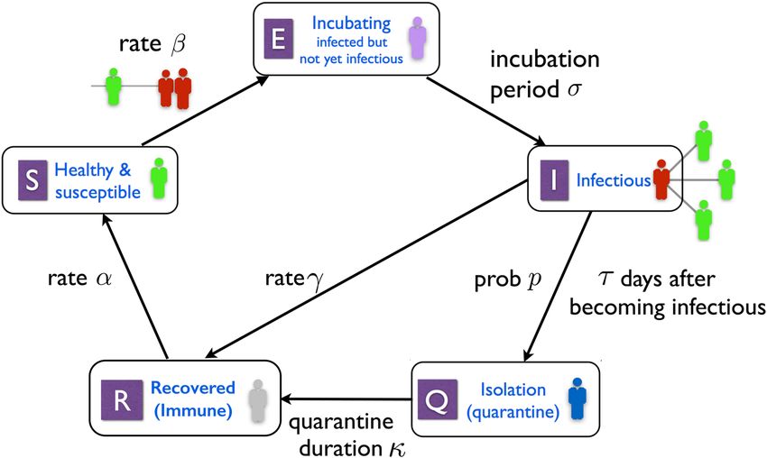
Figure 2. Critical identification time τc is independent incubation σ, isolation time κ and rate of immunity loss
α. Colors represent the asymptotic equilibrium value of infectious individuals Ieq. We consider r = 2.5 and
1/γ = 12 (as for the 2014 Ebola outbreak in Sierra Leone) with full identification probability p = 1. Our predicted
critical time is τc ≈ 6.12 days independent of κ, σ and α, in agreement with simulations. For τ > τc, the disease-
free stable state gives place to an endemic state. Left panel: α versus τ corresponds to the fixed values σ = 2.4
days and κ = 60. Center panel: σ versus τ corresponds to the fixed values κ = 60 days and α = 1/1200. Right
panel: κ versus τ corresponds to the fixed values σ = 2.4 days and α = 1/1200.
we provided a detailed derivation for a simpler model. The results below pertain to the continuum limit system
(1)–(5).
Disease-free states and minimum response needed to squash a small outbreak. Without isola-
tion and assuming everyone is susceptible, whether or not an outbreak will spread is determined by the disease
reproductive number
βm
r= ,
γ
that is, an infection spreads if and only if r > 123. We are interested in the case r > 1, so that if no measures are
taken the infection will spread and reach an endemic state.
Our first result is that when the isolation probability is p and identification time is τ, the effective disease repro-
ductive number rε becomes
rε = r(1 − ε) where ε : = pe−γτ .
The number ε can be thought of as the response capability of the affected community. Upon the sudden appear-
ance of a small group of infected individuals, the incipient epidemic is squashed if and only if r(1 − ε) < 1, i.e., the
isolation protocol as described above reduces the disease reproductive number by rε. This is under the assump-
tion that the outbreak starts near the disease-free equilibrium (S , E, I , Q , R) ≡ (1, 0, 0, 0, 0). The case where a
fraction of individuals is immune to begin with will be discussed later.
We now consider separately the two components in the notion of response capability ε.
Minimum isolation probability. An outbreak can be prevented only if p > pc where
1
pc = 1 − .
r
The number pc is a theoretical minimum: to have a chance to quell the outbreak, health authorities must have
the ability to identify – and the facilities to isolate – a fraction pc of the infectious population immediately after an
individual becomes infectious.
Critical identification time. Possessing the ability to isolate individuals with probability p > pc alone is not
enough; one must be able to identify infectious hosts with sufficient speed. We prove that for each p > pc, there is
a critical identification time
1 p
τc = ln
γ pc
so that the infection dies out if τ < τc.
Observe that in terms of what it takes to squash an outbreak, neither σ, the incubation period, nor α, the
rate of recovery, play a role. The only requirement on κ is that it should be sufficiently long for the individual in
isolation to recover. It is strictly the capability to quickly identify a large enough fraction of the infectious and to
isolate it from the general population.
Figure 2 shows the results of simulations based on the set of delay differential equations above. For illustration,
we consider r = 2.5 and 1/γ = 12 as in the 2014 Ebola outbreak in Sierra Leone (see Table 2). We also consider full
identification probability p = 1. Then, starting from a small number of infected nodes, one observes two distinct
asymptotic regimes: the system tends to a disease-free equilibrium for τ < τc ≈ 6.12 as we have shown; otherwise
it tends to an endemic state. In the left panel, we considered an incubation time σ = 2.4 days and an isolation time
Scientific Reports | (2019) 9:3505 | https://doi.org/10.1038/s41598-019-39714-0 4www.nature.com/scientificreports/ www.nature.com/scientificreports
κ = 60 days, in the middle panel an isolation time κ = 60 days and α = 1/1200. Finally, in the right panel,
α = 1/1200 and σ = 2.4. The demarkation between the two asymptotic regimes is consistent with our analytical
result that critical identification time is independent of incubation time σ, isolation time κ and the rate of immu-
nity acquisition α. Observe though that for τ > τc the asymptotic states do depend on these values.
Predicting critical isolation probabilities and identification times from data. The critical isolation probability
pc and identification time τc = τc(p, r) are readily computed once the disease reproductive number r is known.
Table 2 shows pc and τc for p = 0.8, that is, τc = τc(0.8, r), for several diseases.
As is evident from the data shown, even with the ability to identify 80% of infectious individuals, which
requires considerable resources, the critical identification time τc can be as short as 3 days for severe outbreaks
such as the Spanish Flu and the Ebola in Sierra Leone. That is to say, to prevent such an epidemic from spiraling
out of control, infected individuals must be identified and isolated within 3 days of the end of their incubation
period, which is typically when symptoms begin to appear and not always easy to recognize.
While the critical isolation probability pc depends solely on the basic reproductive number r, the critical delay
depends on both r and γ, so diseases having the same r such as Pertussis and Smallpox can have quite distinct τc.
Recall that r = βm/γ. Among diseases with the same r, for the same value of p > pc, our formula for τc implies that
τc(p) ∝ (βm)−1; that is to say, the delay one can afford is inversely proportional to the transmission rate β of the
disease for m fixed, and inversely proportional to the density of links m for fixed β.
Immunity at the time of an outbreak. The discussion above assumed that at time 0, when the infection first
appears, one is near the disease-free equilibrium (S , E, I , Q , R) ≡ (1, 0, 0, 0, 0); in particular, everyone is sus-
ceptible. We now consider the case where a fraction of the population has immunity at time 0, i.e., R(0) > 0, pos-
sibly from a previous exposure or from vaccination. Assuming α 1, and that the dynamics that determine
whether or not the outbreak can be contained is relatively fast, the situation can be approximated by one in which
R(t ) ≡ R(0) for the time period under consideration. Under these conditions, our results for the case R(0) = 0
together with a rescaling of the total population that participate in the dynamics yields the result that the outbreak
is contained if and only if
1
r(1 − ε) (1 − R(0)) < 1, equivalently, ε > 1 − .
r(1 − R(0))
That is, the effective disease reproductive number is scaled down by a factor of 1 − R(0) as expected. Having
a fraction of the population with immunity allows greater leeway in terms of minimum isolation probability and
critical delay can be computed explicitly as before.
Of major concern is what happens if the response capability is inadequate, that is, if the isolation probability
falls below the required minimum, or if the required identification time is not met. Our next result addresses this
scenario.
Prediction of endemic states. When the response capability as defined above is inadequate, the infection
will persist. That is, for parameters p, τ, κ and σ such that pe−γτ > 1 − 1 , starting from the sudden appearance of
r
a small group of infectious individuals, i.e., from an initial condition near 0 < I 1, S = 1 − I and E = Q = R = 0,
the I-component of the solution will grow; see Methods for more detail. For such initial conditions, we determine
that the solution tends to an endemic equilibrium
1 1
Seq = =
rε r(1 − ε) (6)
(1 − ε)(1 − Seq )
Ieq = −1
γα + γσ + γκε + 1 − ε (7)
γσ
Eeq = Ieq
1−ε (8)
γκε
Qeq = Ieq
1−ε (9)
γα−1
Req = Ieq .
1−ε (10)
A precise statement is as follows: Given p, τ, κ, σ and an initial condition as above, we prove analytically that
there is a unique endemic equilibrium to which the solution can converge, and that this endemic equilibrium
tends to (Seq, Eeq, Ieq, Qeq, Req) given by the formulas above as the initial condition tends to (1, 0, 0, 0, 0). The fact
that orbits starting from near (1, 0, 0, 0, 0) will approach an endemic equilibrium is difficult to prove; this part of
our prediction is supported by numerical simulations. Figure 3 shows the behavior of such solutions tending to
their respective endemic equilibrium, with I > 0.
Observe that ε, the response capability, not only determines whether or not a small outbreak can be contained,
it influences strongly the eventual endemic state when the outbreak happens: Seq, the fraction of the population
Scientific Reports | (2019) 9:3505 | https://doi.org/10.1038/s41598-019-39714-0 5www.nature.com/scientificreports/ www.nature.com/scientificreports
Figure 3. Transient dynamics. (a) Time evolution of epidemic from outbreak to endemic state when isolation
protocol fails. (b) Zoom-in of (a) to show events in the first two cycles. These two panels show the solution
starting from initial condition (S(t), E(t), I(t), Q(t), R(t)) = (1, 0, 0, 0, 0) for t < 0 and (S(0), E(0), I(0), Q(0),
R(0)) = (0.99, 0, 0.01, 0, 0) corresponding to a small initial infection, with parameters r = 2.5, α = 1/1200,
γ = 1/12, σ = 2.4, κ = 60, p = 1 and τ = 12. Panels (c–e) show the dependence of Ipeak, Qpeak (solid lines) and
endemic equilibrium values Ieq, Qeq (dashed lines) on α, σ, and ε respectively. Unspecified parameters are as in
(a and b).
that remains healthy in the eventual endemic steady state, is inversely proportional to (1 − ε), and the fraction Ieq
can be rewritten as
Ieq =
1
(r
r ε
− 1)
=
(1 − ) − ε
1
r
.
γα−1 + γσ + γκε + 1 − ε γα−1 + γσ + γκε + 1 − ε
Observe in the numerators of the quantities above that rε = 1, equivalently 1 − 1 = ε, is the tipping point on
r
one side of which the initial outbreak is contained and on the other the system tends to an endemic equilibrium
with Ieq > 0. While the parameters σ, κ and α appear in the formula for Ieq, hence in Eeq, Qeq and Req as can be seen
in Fig. 2, we observe that the dependence on σ and κ is weak when α 1, that is, when acquired immunity lasts
for a significantly longer time period than incubation, recovery or isolation, which is the case for most diseases.
Assuming that, we have
α 1 2
Ieq = 1 − − ε + O(α ) .
γ r
Here the effect of ε is particularly clear: Since 1 − 1 is the number ε must beat in order to contain the initial
r
outbreak, it can be seen as the minimal response capability required to prevent a full-blown epidemic. We there-
fore have the interpretation that the fraction of infectious in the endemic state is proportional to how far short the
actual response capability ε is from the minimum response needed.
Infection cycles between outbreak and endemic equilibrium. Here we consider the situation where
an outbreak occurs at a time no one in the population has immunity, such as after the disease has vanished for
a couple of generations and suddenly returns, and the response is inadequate for curbing the initial outbreak.
Figure 3(a,b) depict the time evolution of the epidemic from outbreak to near-endemic equilibrium assuming p,
τ, and κ remain fixed throughout. It is evident that the infection occurs in waves, or cycles, at least initially, with
the size of the infection decreasing with each cycle leveling off as it approaches endemic state. It is also quite evi-
dent that even as Ieq is small in the endemic state, the first wave of infection is orders of magnitude worse.
The oscillatory behavior seen is known to occur in the SIRS model23 here it occurs for the same reason: as a
large enough fraction of the population acquires immunity, and immunity is lost at a slow rate, the size of the
susceptible fraction of the population decreases causing the rate of infection, which is proportional to S(t)I(t), to
Scientific Reports | (2019) 9:3505 | https://doi.org/10.1038/s41598-019-39714-0 6www.nature.com/scientificreports/ www.nature.com/scientificreports
slow down – only to flare up again when the R-part of the population rejoins the S-part. What is different here is
that we have assumed a constant response ε, so that for small I(t), the situation is similar to that discussed in the
paragraph on R(0) > 0 in the first part of Results. In particular, if S(t) is such that r(1 − ε)S(t) < 1, the infection
will temporarily abate, to flare up again when S(t) is large enough to bring this quantity above 1. Notice that the
x-axis in Fig. 3(a) is in units t/(τ + σ + κ), so that the timescales for the cycles of infection are significantly longer
than any of these quantities. Rather it is indexed to α and is affected by the fraction of individuals infected during
the course of one cycle. A smaller group is infected in the second cycle than the first because a fraction of the
population is immune at the time of the second outbreak.
We introduce the quantity Ipeak = maxt>0I(t), the maximal fraction of infected individuals that is reached dur-
ing the transient to Ieq; Qpeak is defined analogously. These quantities are of great relevance from the practical
standpoint for health authorities involved in the planning of facilities and care for patients during isolation. To
get our hands on these quantities, we consider first the limiting case where α = σ = ε = 0. In this case, our model
reduces to the classical SIR model, for which we obtain
⁎ 1 1
Ipeak =1− − ln r,
r r
⁎
so that Ipeak can never be larger than 1 − 1 , although a direct connection between Ipeak ⁎
and Ipeak cannot be made.
r
Figure 3(c–e) describe how Ipeak and Qpeak vary as we permit α, σ and ε to become positive. From Fig. 3(c), we see
that while α has a strong effect on Ieq and Qeq, its effect on Ipeak and Qpeak are relatively small, because immunity
loss occurs on a much longer timescale than the time it takes to reach Ipeak or Qpeak. Figure 3(d) shows that both
Ipeak and Qpeak are smaller for diseases with longer incubation periods. This presumably is due to the fact that a
long incubation slows down the rate of infection, while recovery occurs at the same rate. Figure 3(e) shows that
Ipeak decreases as the response is stronger as expected. The dependence of Qpeak on ε is more complicated: In the
figure, τ is fixed and p is increased, i.e., a larger fraction of the infectious is isolated and Qpeak increases with ε for
this interval of ε, but this trend will be reversed as ε continues to increase and Ipeak continues to drop.
Discussion
Isolation of infected hosts disconnects the infection pathway for diseases that are transmitted human-to-human
and should, in principle, be 100% effective, yet it has not always stopped incipient outbreaks from burgeoning into
full-blown epidemics. In this paper we called attention to the fact that a major reason may be “too little, too late”,
meaning the identification of infected hosts may not be sufficiently thorough and are too often subject to delays.
We sought a mathematical model that could offer guidance on the response needed to contain an outbreak, as well
as predict the consequences when one falls short. Our aim was to develop a general theory that is relevant rather
than to carry out detailed studies of specific diseases. Such a model is necessarily a little idealized to be amenable
to (rigorous) mathematical analysis. With these goals in mind we came up with the system of delay differential
equations (1)–(5), the analysis of which produced the results reported here.
We have framed response capability in terms of isolation probability, representing the fraction of the infectious
population that will be identified and isolated, and identification time, the duration an infectious individual can
transmit the disease before being isolated. An isolation strategy can prevent an outbreak only if the response
capability exceeds a minimum threshold value. This was evident in the Ebola outbreak in West Africa, where the
epidemic had started to escalate but reversed course after response capability was increased through international
financial support12.
We have sought to build a theory from first principles. To stress the novelty of this class of models, which
focuses on isolation including the costs of failure in its implementation, we have taken the liberty to name the
class of models considered here SIQ, “Q” for “quarantine”, to distinguish it from standard SIR type models. In
our model, we do not distinguish between isolation and quarantine. We are aware of a different use of the term
“quarantine” in the literature to refer to the isolation of individuals who may have been infected but are not yet
symptomatic4,5.
An interesting direction of research is to consider the isolation of individuals that have been exposed but are
not yet infectious, using for example contact tracing. These strategies have the effect of increasing the isolation
probability, thereby leading to possibility larger tolerable implementation delays. The influence of the underlying
spatial topology of the contact network here was traded off for a clear understanding of the effects of delays in
isolation. The network heterogeneity can strongly influence the dynamics24 and it can either be tackled by means
of heterogeneous mean field approximation25,26, or by a direct study of networks with adaptive change of the
structure due to network rewiring caused by the isolation protocol27. Such approaches should enable one to clarify
the role of highly connected nodes in the isolation protocol.
Methods
Dynamical Systems Framework. Here we present a mathematical framework for the study of the delay
system (1–5) 20. Time delay implies that this system is infinite-dimensional, i.e. its state can be described by the
history function, where the variables S, I, E, Q, R are prescribed on an interval of the length σ + τ + κ of maximal
time delay. More specifically, let : = C([ − σ − τ − κ , 0], 5) be the Banach space of 5-valued continuous
functions with the sup-norm. Given an initial function φ ∈ , the solution x(t , φ) ∈ 5, t ≥ 0, to the initial value
problem exists and is unique20. Using the notation
x t(φ) = x(t + θ , φ), θ ∈ [ − σ − τ − κ , 0],
it is known that T t : φ x t(φ) defines a C1 semi-flow on .
Scientific Reports | (2019) 9:3505 | https://doi.org/10.1038/s41598-019-39714-0 7www.nature.com/scientificreports/ www.nature.com/scientificreports
The conservation of mass property, namely S′(t) + E′(t) + I′(t) + Q′(t) + R′(t) = 0 for all t ≥ 0, implies that if
φ = (φS, φE, φI, φQ, φR) and x(t; φ) = (S(t), E(t), I(t), Q(t), R(t)), then S(t) + E(t) + I(t) + Q(t) + R(t) = φS(0) + φE(0
) + φI(0) + φQ(0) + φR(0) for all t ≥ 0. To obtain biologically relevant solutions we further restrict to the subset on
which S(t), E(t), I(t), Q(t), R(t) ≥ 0.
In Results, we considered initial conditions φ representing the sudden appearance of a small group of infec-
tious individuals. These initial conditions should be near (1, 0, 0, 0, 0), the disease-free equilibrium with constant
coordinate functions. Two examples are (i) φ = (φS, φE, φI, φQ, φR) where φS = 1 − c, φI = c and φE = φQ = φR = 0,
all constant functions with 0 < c 1, and (ii) φ(t) = (1, 0, 0, 0, 0) for t < 0 and φ S(0) = 1 − c, φ I(0) = c,
φE(0) = φQ(0) = φR(0) = 0. While such a φ is not in , T t(φ) ∈ for t ≥ σ + τ + κ.
Numerically, DDEs are solved using the method of steps: Given an initial function φ we obtain the solution x(t, φ)
to the DDE in the interval [0, τ + σ + κ] as the solution of the nonautonomous Ordinary Differential Equation using a
4th order Runge-Kutta with integration step 10−3 where the initial function is a known time-dependent input.
Disease-free states. For fixed α, σ, p, τ and κ, the set of initial conditions φ for which all component
functions are constant and φI is identically equal to zero defines the “disease-free” equilibria. These comprise the
two-parameter family of constant functions (S(t), E(t), I(t), Q(t), R(t)) = (S(0), E(0), 0, Q(0), 0) for all t, where
S(0) + E(0) + Q(0) = 1. To investigate the stability of a given equilibrium solution, we linearize the system to
obtain the following quasi-polynomial characteristic equation
χ(λ) = λ2(λ + α) (λ + γ − βme−σλ(1 − εe−τλ )S(0)) = 0.
Two zero eigenvalues correspond to directions along the manifold of equilibria. An analysis shows that all
disease-free equilibria are linearly stable if S(0) ≤ 1/r(1 − ε), and unstable otherwise. At this bifurcation value,
a third eigenvalue crosses the imaginary axis with nonzero speed and gives rise to a different class of endemic
(nonzero infected) equilibria. If S(0) ≤ 1/r(1 − ε) no further bifurcations occur, so that these disease-free equilib-
ria are linearly stable independently of the incubation time and isolation protocol.
The analysis above is carried out for fixed α, σ, p, τ and κ. We now turn the question around and ask for which
values of these parameters is (S , E, I , Q , R) ≡ (1, 0, 0, 0, 0) a stable equilibrium. This is how the minimum iso-
lation probability pc and critical identification times τc(p) announced in Results were deduced.
Endemic states. In addition to the disease-free states, system (1)–(5) possesses a two-parameter family of
endemic equilibria consisting of constant functions (S(t), E(t), I(t), Q(t), R(t)) = (Seq, E(0), I(0), Q(0), γα−1I(0)/
(1 − ε)) with I(0) > 0, Seq = 1/rε and
γα−1
Seq + E(0) + Q(0) + 1 + I (0) = 1,
(1 − ε) (11)
where I(0) and Q(0) can be considered as the free parameters. One sees immediately that Seq is not affected by the
recovery rate α, the incubation period σ and isolation time κ. In particular, it is constant for the whole family of
endemic equilibria. The linear stability analysis of these equilibria is very challenging from an analytical point of
view. They are stable for reasonable values of κ, destabilizing as κ increases. A detailed analysis will be published
elsewhere. The formal limiting case α → ∞ (immediate waning of immunity) has been studied in detail22.
The main concern of this paper is the effect of isolation on disease outcome starting from a small outbreak. To
this end, the following conserved quantities will be of major help:
0
HE(φ) = φE(0) − βm∫−σ φS(θ)φI(θ) dθ
−σ − τ
HQ(φ) = φQ(0) − βmε ∫ φS(θ)φI(θ) dθ
−σ − τ − κ
The conservation of these quantities along solutions d HE , Q(x t(φ)) = 0 can be proved by direct computation.
dt
Restricting our attention to initial functions of the type (1, 0, 0, 0, 0) for t ∈ [ − τ − σ − κ , 0) and (1 − I0(0), 0,
I0(0), 0, 0) at t = 0 for some I0(0), we have HE,Q(xt(φ)) = HE,Q(φ) = 0. This implies
t
E (t ) = β m ∫t−σ S(θ)I (θ)dθ, (12)
t −σ −τ
Q(t ) = βmε ∫t−τ−σ−κ S(θ)I (θ)dθ. (13)
Equations (12) and (13) can be used to find the corresponding endemic equilibrium (Seq, Eeq, Ieq, Qeq, Req)
reached from the considered initial function. More specifically, we determine Eeq = βmσSeqIeq and Qeq = βmεκSe-
qIeq. Inserting these values in Eq. (11), we obtain Ieq, and, hence, the unique endemic equilibrium (6)–(10).
References
1. Woolhouse, M. E., Brierley, L., McCaffery, C. & Lycett, S. Assessing the epidemic potential of rna and dna viruses. Emerg Infect
Diseases 22, 2037 (2016).
2. Tian, H. et al. Avian influenza h5n1 viral and bird migration networks in asia. PNAS 112, 172–177 (2015).
Scientific Reports | (2019) 9:3505 | https://doi.org/10.1038/s41598-019-39714-0 8www.nature.com/scientificreports/ www.nature.com/scientificreports
3. Center for Disease Control & Prevention. Legal authorities for isolation and quarantine, https://www.cdc.gov/quarantine/pdf/legal-
authorities-isolation-quarantine.pdf.
4. Siegel, J. D., Rhinehart, E., Jackson, M. & Chiarello, L. 2007 guideline for isolation precautions: preventing transmission of infectious
agents in health care settings. Am J Infect Control 35, S65–S164 (2007).
5. Center for Disease Control & Prevention. Announcement: Interim us guidance for monitoring and movement of persons with
potential ebola virus exposure. MMWR Morb Mortal Wkly Rep 63, 984 (2014).
6. Zuzek, L. A., Stanley, H. & Braunstein, L. Epidemic model with isolation in multilayer networks. Sci Rep 5, 12151 (2015).
7. Grigoras, C. A., Zervou, F. N., Zacharioudakis, I. M., Siettos, C. I. & Mylonakis, E. Isolation of C. difficile carriers alone and as part
of a bundle approach for the prevention of Clostridium Difficile Infection (CDI): A mathematical model based on clinical study
data. PLOS One 11, 1–12 (2016).
8. Reppas, A. I., Spiliotis, K. G. & Siettos, C. I. Epidemionics: from the host-host interactions to the systematic analysis of the emergent
macroscopic dynamics of epidemic networks. Virulence 1, 338–349 (2010).
9. Day, T., Park, A., Madras, N., Gumel, A. & Wu, J. When is quarantine a useful control strategy for emerging infectious diseases? Am
J Epidemiol 163, 479–485 (2006).
10. Fraser, C., Riley, S., Anderson, R. M. & Ferguson, N. M. Factors that make an infectious disease outbreak controllable. PNAS 101,
6146–6151 (2004).
11. Peak, C. M., Childs, L. M., Grad, Y. H. & Buckee, C. O. Comparing nonpharmaceutical interventions for containing emerging
epidemics. PNAS 114, 4023–4028 (2017).
12. Kucharski, A. J. et al. Measuring the impact of ebola control measures in sierra leone. PNAS 112, 14366–14371 (2015).
13. Herstein, J. J. et al. Sustainability of high-level isolation capabilities among us ebola treatment centers. Emerg Infect Diseases 23, 965
(2017).
14. Team, W. E. R. Ebola virus disease in west africa - The first 9 months of the epidemic and forward projections. N Engl J Med 2014,
1481–1495 (2014).
15. Donnelly, C. A. et al. Epidemiological determinants of spread of causal agent of severe acute respiratory syndrome in hong kong.
Lancet 361, 1761–1766 (2003).
16. Pereira, T. & Young, L. S. Control of epidemics on complex networks: Effectiveness of delayed isolation. Phys Rev E 92, 4–7 (2015).
17. Reppas, A. I., Tsoumanis, A. C. & Siettos, C. I. Coarse-grained bifurcation analysis and detection of criticalities of an individual-
based epidemiological network model with infection control. Appl. Math. Model. 34, 552–560 (2010).
18. Lu, K., Wang, Q. D. & Young, L.-S. Strange attractors for periodically forced parabolic equations. AMS Memoirs 223, 1054 (2013).
19. Guckenheimer, J & Holmes, P. Nonlinear oscillations, Dynamical Ssystems, and Bifurcations of vector fields Applied Math Sc. Vol. 42
(Springer, 2002).
20. Hale, J. K & Lunel, S. M. V. Introduction to Functional Differential Equations, Applied Mathematical Sciences Vol. 99 (Springer New
York, New York, NY, 1993).
21. Yanchuk, S. & Giacomelli, G. Spatio-temporal phenomena in complex systems with time delays. J Phys A Math Theor 50, 103001
(2017).
22. Ruschel, S., Pereira, T., Yanchuk, S. & Young, L.-S. SIQ: a delay differential equations model for disease control via isolation. arXiv
preprint arXiv:1804.02696 (2018).
23. Brauer, F. & Castillo-Chavez, C. Mathematical models in population biology and epidemiology, Texts in Applied Mathematics Vol. 40
(Springer, 2012).
24. Kuperman, M. & Abramson, G. Small world effect in an epidemiological model. Phys. Rev. Lett. 86, 2909–2912 (2001).
25. Barthélemy, M., Barrat, A., Pastor-Satorras, R. & Vespignani, A. Dynamical patterns of epidemic outbreaks in complex
heterogeneous networks. J Theor Biol 235, 275–288 (2005).
26. Hayashi, Y., Minoura, M. & Matsukubo, J. Oscillatory epidemic prevalence in growing scale-free networks. Phys. Rev. E 69, 016112
(2004).
27. Shaw, L. B. & Schwartz, I. B. Fluctuating epidemics on adaptive networks. Phys. Rev. E 77, 066101 (2008).
28. Althaus, C. L. Estimating the Reproduction Number of Ebola Virus (EBOV) During the 2014 Outbreak in West Africa. PLOS Curr
Outbreaks pp. 1–12 (2014).
29. Müller, J. & Kuttler, C. Methods and Models in Mathematical Biology. 1 edition, (Springer-Verlag, Berlin, Heidelberg, 2015).
Acknowledgements
This paper was developed within the scope of the IRTG 1740/TRP 2015/50122-0, funded by the DFG/FAPESP.
L.-S.Y. was partially supported by NSF Grant DMS-1363161. T.P. was partially supported by FAPESP grant
2013/07375-0 and Serrapilheira grant G-1708-16124. T.P. and S.R. thank the Courant Institute for the hospitality.
Author Contributions
All authors carried out the research. L.-S.Y. and T.P. wrote the main body of the manuscript. All authors wrote and
edited the manuscript. S.R. and T.P. conducted numerical experiments. L.-S.Y. designed Figure 1, T.P. prepared
Figures 1 and 2 and S.R. and S.Y. prepared Figure 3.
Additional Information
Competing Interests: The authors declare no competing interests.
Publisher’s note: Springer Nature remains neutral with regard to jurisdictional claims in published maps and
institutional affiliations.
Open Access This article is licensed under a Creative Commons Attribution 4.0 International
License, which permits use, sharing, adaptation, distribution and reproduction in any medium or
format, as long as you give appropriate credit to the original author(s) and the source, provide a link to the Cre-
ative Commons license, and indicate if changes were made. The images or other third party material in this
article are included in the article’s Creative Commons license, unless indicated otherwise in a credit line to the
material. If material is not included in the article’s Creative Commons license and your intended use is not per-
mitted by statutory regulation or exceeds the permitted use, you will need to obtain permission directly from the
copyright holder. To view a copy of this license, visit http://creativecommons.org/licenses/by/4.0/.
© The Author(s) 2019
Scientific Reports | (2019) 9:3505 | https://doi.org/10.1038/s41598-019-39714-0 9You can also read