Cooperation dynamics under pandemic risks and heterogeneous economic interdependence - arXiv
←
→
Page content transcription
If your browser does not render page correctly, please read the page content below
Cooperation dynamics under pandemic risks and heterogeneous economic
                                                                             interdependence

                                                                     Manuel Chicaa,b,∗, Juan M. Hernándezc , Francisco C. Santosd
                                                              a
                                                               Andalusian Research Institute DaSCI “Data Science and Computational Intelligence”,
                                                                                    University of Granada, 18071 Granada, Spain
                                                                                 b
                                                                                   School of Electrical Engineering and Computing,
                                                                          The University of Newcastle, Callaghan, NSW 2308, Australia
                                                                     c
                                                                       Department of Quantitative Methods in Economics and Management,
                                                                Universtiy Institute of Tourism and Sustainable Economic Development (TIDES),
arXiv:2108.00886v1 [physics.soc-ph] 30 Jul 2021

                                                                      University of Las Palmas de Gran Canaria, 35017 Las Palmas, Spain
                                                         d
                                                           INESC-ID & Instituto Superior Técnico, Universidade de Lisboa, 2744-016 Porto Salvo, Portugal

                                                  Abstract

                                                     The spread of COVID-19 and ensuing containment measures have accentuated the profound
                                                  interdependence among nations or regions. This has been particularly evident in tourism, one of the
                                                  sectors most affected by uncoordinated mobility restrictions. The impact of this interdependence
                                                  on the tendency to adopt less or more restrictive measures is hard to evaluate, more so if diversity
                                                  in economic exposures to citizens’ mobility are considered. Here, we address this problem by
                                                  developing an analytical and computational game-theoretical model encompassing the conflicts
                                                  arising from the need to control the economic effects of global risks, such as in the COVID-19
                                                  pandemic. The model includes the individual costs derived from severe restrictions imposed by
                                                  governments, including the resulting economic interdependence among all the parties involved in
                                                  the game. By using tourism-based data, the model is enriched with actual heterogeneous income
                                                  losses, such that every player has a different economic cost when applying restrictions. We show
                                                  that economic interdependence enhances cooperation because of the decline in the expected payoffs
                                                  by free-riding parties (i.e., those neglecting the application of mobility restrictions). Furthermore,
                                                  we show (analytically and through numerical simulations) that these cross-exposures can transform
                                                  the nature of the cooperation dilemma each region or country faces, modifying the position of the
                                                  fixed points and the size of the basins of attraction that characterize this class of games. Finally, our
                                                  results suggest that heterogeneity among regions may be used to leverage the impact of intervention
                                                  policies by ensuring an agreement among the most relevant initial set of cooperators.
                                                  Keywords: Collective risk dilemma; Economic interdependence; Pandemic risks; COVID-19;

                                                                                                        1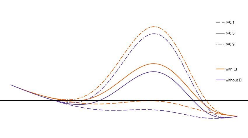
Evolutionary game theory;

1. Introduction

       The COVID-19 pandemic has caused the most severe global economic breakdown of the recent
history, mainly due to the measures to control the virus spread (e.g., quarantines, stay-at-home
and social distancing policies), which have produced a dramatic shutdown of the economic activity.
In this context, the coordination among countries is an essential instrument to efficiently control
pandemic and enhance economic recovery [35, 17].
       The pandemic control measures result in two types of negative economic effects on countries
and regions. First, the direct effects, derived from internal mobility restrictions, which seriously
injure many sectors in the country. They do not just include hospitality and entertainment, but
also banks, stock market and education sector [25]. Second, indirect effects, induced by trade
and financial linkages among countries, which produce economic contagion of the consequences of
restrictions in a country to a foreign linked country [25, 13]. An example of an indirect effect is
the travel restrictions in tourist dependent countries, which produce a serious economic loss to
destination countries [31]. Other pandemic consequences are found in international supply chains.
Thus, export-oriented countries are influenced by demand shortfall of the importing countries and,
at the same time, supply disruption from some countries such as China produces input shortages
and inflationary pressure in import-countries [28]. In addition, the contact pattern in some regions
are influenced by the social distancing policies followed in others [17]. All this phenomena stem
from the economic interdependence (EI) among countries.
       Furthermore, the economic impact of the pandemic control measures is not homogeneous for
all the countries and regions. Those service and export-oriented countries, such as those depending
on tourism, entertainment and transport, have been more affected than others [4]. For example,
Panama, which depends mainly on tourism and transport services, suffered a serious GDP decrease
in 2020 (19%), and other many tourism-dependent small-islands states, such as Maldivas, Fiji
and Bahamas, experimented similar economic consequences. In Europe, the COVID-19 pandemic

   ∗
    Corresponding author
    Email addresses: manuelchica@ugr.es (Manuel Chica ), juan.hernandez@ulpgc.es (Juan M. Hernández),
franciscocsantos@tecnico.ulisboa.pt (Francisco C. Santos)

Preprint submitted to Elsevier                                                              August 3, 2021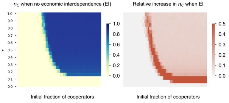
economic loss in Spain, around 10% decrease of the GDP, duplicated the economic loss in Germany.
These evidences show that the economic consequences of the implementation of control measures
are markedly heterogeneous.
   The coordination problem of pandemic control measures can be represented through a collective-
risk dilemma (CRD) [22, 33]. This is a multiplayer public good game (PGG) where every player can
contribute with some amount to avoid a certain risk of failure. Normally, it is not necessary that all
players contribute to achieve the common goal and there is some space for free-riders who benefit
from the others’ contribution. Traditionally, cooperation to mitigate climate change by cutting
carbon emissions has been one of the most important applications of CRDs [37, 21, 1, 27, 42, 14, 10].
More recently, CRDs have been proposed for the coordination of restrictions and reopen policies
in the current context of the COVID-19 pandemic [7].
   The aim of our study is to analyze the conditions for achieving coordination among countries
to control pandemic situations, taking into account the specific economic consequences of these
measures. Specifically, we propose a new CRD model where EIs among the players are considered
by altering the expected profits by regions given the restrictions applied by cooperating regions.
The proposed CRD model also incorporates the heterogeneity found for regions and countries with
respect to their income loss when cooperating by restricting the economic activity. Heterogeneity is
omnipresent in reality but only few studies included heterogeneous features in social dilemmas [19].
   We fit a log-normal distribution for feeding the model with heterogeneous economic loss values
by analyzing real data from tourism contribution to GDP of the European Union NUTS2 regions.
The experiments comprise the evaluation of the final cooperation levels of the population with
and without EI and validate them under the presence of heterogeneity. Our results show that the
existence of EI among countries can favor cooperation for all the tested conditions. To understand
the reason behind these observations, we extract the stable and unstable points of the new dilemma
with and without heterogeneity. To this end, we propose a new way of calculating the internal
roots from the agent-based simulation results.
   Finally, we take advantage of the reality coming from the income loss heterogeneity of the
model to analyze those initial conditions facilitating cooperation. Three scenarios are evaluated.
We first set the initial cooperators at random but we also condition those initial cooperators by a
positive and negative bias by they income losses of the regions. The reader will see how significant

                                                  3
differences in the final cooperation levels are achieved when choosing the best initial conditions
alternative. These results will help to engineer more effective governmental policies to increase
cooperation.
2. Model
We present a CRD model to represent the cooperation game among regions or countries (we
call them countries from now on) when adopting measures to control pandemic spread having
into account their negative economic consequences. We resort to evolutionary game theory and
stochastic population dynamics [16, 34, 24, 38, 23, 30, 29] when required, combined with agent-
based computer simulations [20, 2]. The inspiration for this model was found in previous CRD
models for cooperative actions against climate change [33, 42] and pandemic spread [7].
2.1. Game definition including economic interdependence (EI)
The model includes a finite number Z of countries or regions. Every player i can choose two
strategies si (t) at every time step t: cooperation (C), which means adopting measures to control
the pandemic spread and suffering income loss; and defection (D), which means not adopting any
measure, continuing with the normal economic activity and eventually free-riding the correct public
health conditions derived from others’ cooperation.
Players interact in groups of size N , representing international or regional agreements, alliances
or work-groups. By assumption, these groups are randomly formed. Every group faces a risk
r ∈ [0, 1] for the health care system to collapse and the resulting economic breakdown, if the
epidemic is not controlled enough inside the group. This happens when the number of cooperators
in the group does not achieve a minimum M ≤ N . When the number of cooperators is equal or
higher than M in a group of size N countries, the pandemic is under control and the economic
breakdown is not produced.
When a country i cooperates, economic activity critically stops and an income loss ci occur
in the region ought to these restrictions. This loss is not necessarily constant throughout the
population, but every country has its loss value, which depends on the specific economic structure
of the country. In addition, the economic breakdown in the cooperator i is spread to the rest of
countries due to the international economic linkages among them. Thus, defector countries are not
free of economic negative spillovers or contagion from other countries. Instead, they are influenced
4by the number of cooperators in the total population. The more the cooperator countries in the
total population, the higher the negative economic consequences in the defector country.
The conditions above are represented in the expected payoff ΠiD (ΠiC ) of a defector (cooperator)
country i. They are:
k
ΠiD (j)= 1 − ci [Θ(j − M ) + (1 − r) (1 − Θ(j − M ))], (1)
Z
i i k
ΠC (j) = ΠD (j) − 1 − ci , (2)
Z
where j is the number of cooperators in the group and k is the number of cooperators in the total
population. The variable M = mN , where N is the group size and m is the minimum fraction
of cooperators to avoid collapse. The Heaviside step function Θ(x) is equal to 0 whenever x < 0
and equal to 1 otherwise. The initial endowment or maximum payoff obtained in absence of any
pandemic is normalized to 1.
The first term of Equation 1 shows that when the number of cooperators in the group is above
the threshold M , the expected payoff of a defector is not maximum, but lowers an amount due
to the economic interdependence with cooperator countries. Specifically, the loss of the defector’s
k
income is a fraction Z of its own maximum loss ci . This term ci Zk is added to the cooperator’s
payoff (Equation 2) since we assume that the single cost of cooperation ci already includes the
economic contagion derived from international linkages. The total loss in the cooperators’ income
is ci , as expected. When the necessary number of cooperators in a group is not achieved (j < M ),
both cooperators and defectors have a risk r of global economic collapse and null economic activity.
2.2. Individual update of the game strategies
After playing a game round t, players can update their strategies according to the received
payoffs. Here, we have considered the Fermi function as the evolutionary update rule [36, 39]. The
Fermi rule is a stochastic pairwise comparison rule in which strategies that do well, are more likely
to be imitated, and spread throughout the population. In detail, at each time-step, a player i
with a payoff Πi is randomly selected from the population for strategy revision. Player i will then
randomly select another player j from the population as a potential role model; i will imitate the
strategy of j with a probability p that increases with their payoff difference — (Πj − Πi ) — and
can be written as in [38]:
51
p= . (3)
1+ e−β(Πj −Πi )
The free parameter β is the intensity of selection, encoding the chance of mistakes during the
imitation process. This means that a player i can copy another player’s strategy j despite having
a lower payoff. We set β = 1 in all the experiments of the study. Additionally, the players of
the game can randomly explore other strategies, adopting a strategy at random with probability
1
µ. This mutation (or exploration) probability (µ) equals Z in all experiments. This update rule
can be used in both synchronous and asynchronous paradigm. We have confirmed via numerical
simulations that our conclusions remain valid for both cases.
2.3. Stochastic population dynamics
Let us start by assuming that the income loss ci is homogeneous for all players. Then we
have a unique income loss c for all countries and the payoff derived from any strategy depends on
the general parameters and the number of cooperators j in the group. Let us also assume that
all players are equally likely to interact, a configuration known as a well-mixed population [34].
In other words, we have a random selection of partners to form groups. In this limit, we can
analytically compute the expected payoff (or fitness) of a cooperator/defector for a given number
of cooperators k in the population by using an hyper-geometric sampling [15, 26]:
−1
N −1
Z −1 X k−1 Z −k
fC (k) = ΠC (j + 1),
N −1 j=0 j N − j − 1
−1
N −1
Z −1 X k Z −k−1
fD (k) = ΠD (j),
N −1 j=0 j N −j−1
where we have removed the super-index referring to player i in the payoff functions.
The update rule described in section 2.2 defines a Markov process where, at every time step,
the probability to increase the number of cooperators k in the population is [38],
+ Z −k k 1
T (k) = (1 − µ) +µ , (4)
Z Z 1 + e−β(fC (k)−fD (k))
and the probability to decrease the number of cooperators is
− k Z −k 1
T (k) = (1 − µ) +µ . (5)
Z Z 1 + e−β(fD (k)−fC (k))
6Several tools can be used to analyze the evolutionary dynamics emerging from this ergodic
Markov chain. First, the gradient of selection [26, 33], G(k) = T + (k) − T − (k), indicates the
direction of change for every cooperation level. Second, as the process includes probabilistic mu-
tation (µ), the population does not fixate in any stationary state. Thus, instead of computing
the probability of fixation in each absorbing state, we can make use of the stationary distribution
of this Markov chain to analyze the asymptotic state of the population, and assess the perva-
siveness in time of a each fraction of cooperators. To this end, we build the transition matrix
M = (pij )(Z+1)×(Z+1) , where pk,k±1 = T ± (k), pk,k = 1 − pk,k+1 − pk,k−1 and 0 for the rest. This
is a tridiagonal matrix and the stationary distribution is the normalized eigenvector (p̄k )k=0..Z
corresponding to eigenvalue 1 of the transpose of matrix M . Third, the expected final number of
cooperators is calculated from the stationary distribution, as nC = Z
P
k=0 p̄k k. We can also use
the hypergeometric distributions above to calculate the probability aG (k) of having groups with
M cooperators or more for every cooperation level k [41, 42]. This is given by ηG = Z
P
k=0 p̄k aG (k)
indicating the average group achievement of the game in the stationary solution.
2.4. Agent-based computer simulations
While convenient for the case with homogeneous income losses (c), the analytical mean-field
approach described above is no longer valid in the case of heterogeneous exposures or losses. The
inclusion of regions or countries’ diversity in exposure introduces a higher level of complexity may,
nonetheless, be conveniently described through Monte-Carlo (MC) agent-based simulations [20,
2], performed in computer clusters and resorting to parallel computing architectures. Evolution
proceeds in discrete steps involving imitation and mutation, in line with the stochastic dynamics
described above.
We fix the size of the groups N to 10 and the minimum threshold m to 0.7 (i.e., M = 7) for
the whole set of experiments shown in the study. Experiments with group sizes N = {5, 10, 25}
and m = {0.5, 0.7} were carried out without noticing significant changes. For the sake of numerical
tractability, the size of the population in the analytical results is Z = 200. For the agent-based
simulations, the size of the population is Z = 2.0 × 10³ and we run the model for 30 independent
MC realizations and a maximum number of 103 synchronous time-steps, where all the realizations
reach a stationary stable state and deviation from the MC realizations is low. Finally, all the
simulation results were obtained by averaging the last 25% of the simulation time-steps in the
7independent MC runs.
3. Results and discussion
In this section we analyze the results of three different experiments by considering the effects
of the economic interdependence (EI) in the dilemma. First, we present the analytical study of the
game when having homogeneous costs c in Section 3.1. We later apply agent-based simulations
to the dilemma with costs heterogeneity (Section 3.2) and study the roots of the dilemma in
Section 3.3. Finally, Section 3.4 provides guidance on how to engineer interventions for increasing
cooperation by taking into account heterogeneity.
3.1. Analytical study of the cooperation increase when considering EI
First, we analyze the effect of the income loss on the final stationary state of the game. Figure
1 shows the average final percentage of cooperators as a function of the homogeneous income loss
c for three risk levels. To analyze the effect of economic interdependence (EI), we represent the
trajectories with two models: one adopting the payoff equations 1 and 2 (model with EI) and other
one using the same equations but removing the term ci Zk (model without EI).
1.00
fraction of cooperators (nC)
0.75
0.50 with EI
without EI
0.25
0.00
0.0 0.1 0.2 0.3 0.4
income loss (c)
Figure 1: Final fraction of cooperators for different values of homogeneous income loss c for the models with economic
interdependence (EI) and without EI. We assume three risk levels. This figure shows that EI increases the levels of
cooperation and group success for wide intervals of income losses and risk values. The parameter values are: Z = 200,
N = 10, M = 7, β = 1, µ = 1/Z.
8As it can be observed, the income loss negatively influences on the final number of cooperators.
In general, its effect is not strong for income loss values near zero, but up to a certain threshold,
the expected number of cooperators dramatically decreases until achieving almost null values. The
lower the risk associated with the game, the lower the levels of income loss where null cooperation
is achieved.
Moreover, Figure 1 shows the positive effect of EI on the cooperation in the three risk levels
shown. Therefore, the existence of economic linkages among countries in the pandemic context
favors cooperation in the dilemma. The gap in the number of cooperators between the two models
is larger for larger risk values. This result is apparently counter-intuitive, since including new
economic costs to the players may in general deter the disposition to cooperate. However, this is
not the case in this context, since the income loss due to EI reduces the overall economic benefit
at stake for all players and therefore shortens the benefit margin of being defector.
0.03
Gradient of selection, G(k)
with EI
without EI
0.02 unstable
stable
0.01
0.00
-0.01 xL xR
0.0 0.25 0.5 0.75 1.0
fraction of cooperators, k/Z
Figure 2: Gradient of selection for the models with and without EI. According to the sign of the Gradient of selection
G(k), cooperators (defectors) are likely to increase in the population whenever G(k) > 0 (G(k) < 0). We assume
the same three risk levels as in Figure 1. EI is able to transform the overall dynamics, by reducing the coordination
requirements (xL ) required to reach a cooperative basin of attraction. Similarly, EI also increases the stable fraction
of cooperation (xR ) reached whenever xL is overcome. Parameter values: Z = 200, N = 10, M = 7, β = 1, µ = 1/Z.
A deeper insight of the analytical solution of the model with and without EI is presented in
Figure 2, which shows the gradient of selection G(k) for the same three risk levels in Figure 1, with
and without EI. If the gradient of selection, G(k), is positive (negative), the number of cooperators
is likely to increase (decrease) whenever the population has k cooperators. The roots of G(k) offer
9the finite population analogues of fixed points in infinite populations [26, 33]. Here, we can identify
configurations with two internal roots typical of this class of dilemmas: one unstable root on the
left-hand side (xL ) and one stable root (xR ) for higher fractions of cooperators, associated with
two well-defined basins of attraction. It also suggests that a critical mass of cooperators (xL ) needs
to be surpassed such that the system naturally self-organizes into a co-existence of cooperators and
defectors.
Interestingly, the gradients in Figure 2 show that stable equilibria (xR ) occur for higher levels
of cooperators when EI is included. At the same time, the coordination point (xL ) tends to move
towards lower values of the fraction of cooperators k/Z when EI is in place. This suggests that
EI reduces the requirements to sway to the cooperative basin of attraction where cooperators and
defectors may co-exist. Naturally, the position of both (xL ) and xR depends on the value of risk
(r). The higher the perception of the risk, the lower the unstable equilibrium xL and the higher
the stable equilibrium xR , being more likely to overcome the dilemma. The position of these roots
— but also the amplitude of G(k) — determine the final stationary distribution and the expected
prevalence of cooperators. Finally, the exploration (or mutation) probability (µ) drive the system
to the center of the cooperation axis by making G(0) > 0, further favouring the shift towards the
right-hand side of the simplex.
3.2. Simulation-based results for heterogeneous income losses based on real data
As commented in the introduction, the income loss due to the implementation of pandemic
control measures is not homogeneously distributed among countries. For example, tourism was
one of the most affected sectors by the COVID-19 pandemic and tourism GDP contribution of
the European regions is one example of the heterogeneity of the players involved, as discussed
in [7]. The number of regions in the EU NUTS2 classification [12] is 312 and we use real data
from this classification to compute the exposure of the regions to a lockdown and tourism activity
halt. The considered indicator for this contribution are the nights spend at tourist accommodation
establishments per inhabitant. Although the averaged contribution of the regions is 0.04, we
observe a clear heterogeneity in the distribution. Figure 3 shows the 312 data points and two fitted
distribution: a log-normal and a power-law.
The log-normal distribution with fitted parameters µln = −4.39 and σln = 1.63 is the one
with the best fitting. Therefore, we use this distribution to feed the costs or income loss ci for
101
cumulative probability
0.1
0.01
0.001
10-4 10-3 10-2 10-1 1
tourism-dependence ratio
Figure 3: Cumulative distribution of the income loss for the 312 regions of the EU NUTS2 (circles). It shows that
regions’ typically portray a significant heterogeneity in the dependence from tourism activity. Blue solid line represent
the fitted log-normal distribution and the dashed line the fitted Pareto distribution (see main text for details).
the players. Because of the heterogeneity in the costs, it is not possible to fully assess the overall
dynamics through the mean-field analysis of the previous section. Thus, in the following, we resort
to agent-based simulations to estimate the evolutionary dynamics of the model [2, 7]. We have
tested both log-normal and power law distributions of potential income losses without significant
changes and therefore, the same conclusions apply for both distributions.
Figure 4 shows the averaged final cooperation frequency for the game with and without EI
using the log-normal distribution of income loss. To obtain each point of both curves at every
risk value, we average the simulations results from a set of sufficient discrete values for the initial
frequency of cooperators of the system, n0C .
We can see in this figure how the increase in cooperation is clear for all the risk levels after
averaging all the possible initial conditions of cooperation. The inclusion of EI boosts cooperation
even for very low risk values and the positive gap in cooperation remains practically equal for the
whole range of risk values. Therefore, we see that the main behavior of the system is the same
when injecting heterogeneity through the real distribution of income loss ci . The results are in
line with the homogeneous setting of the model. The global increase in final cooperation when
incorporating EI in the dilemma is robust, independently from the heterogeneity of the income
loss.
11Figure 4: Final fraction of cooperators nC for different risk levels r comparing the dilemma with and without
economic interdependence when having heterogeneous income loss from a fitted log-normal distribution. Economic
interdependence (EI) leads to high levels of cooperation, even when regions portray a large diversity in economic
exposure to confinement measures. Results obtained via numerical simulations with Z = 2 × 10³ , N = 10, M = 7,
β = 1, and µ = 1/Z.
3.3. Study on the internal fixed points of the game
The adoption of a different exposure for each agent makes it hard to assess the overall dynamics
from an analytical perspective. Particularly, the inference of the effective gradient of selection and
associated equilibrium from large-scale computer simulations is not always trivial (see, e.g.,[32]).
In this section we aim at explaining why there is an increase in cooperation when simulating the
model with heterogeneous costs and estimate the roots of the dynamics as in the analytical model.
Therefore, we first propose a methodology to estimate, from the sensitivity analysis on risk r and
initial cooperators n0C , the stable and unstable equilibrium points. Figure 5 shows this sensitivity
analysis on r and n0C where each cell is the averaged final frequency of cooperators nC from the
MC realizations of the agent-based model using the log-normal distribution of income loss ci . The
12plot on the left represents the absolute nC values of the game without EI while the plot on the
right shows the relative increase in nC of the game including EI with respect to the traditional
dilemma.
nC without EI Relative increase in nC with EI
1.0
0.8
0.6
risk, r
0.4
0.2
0.0
0.0 0.5 1.0 0.0 0.5 1.0
initial fraction of cooperators initial fraction of cooperators
Figure 5: Heatmaps comparing the sensitivity analysis on r and the initial fraction of cooperators when having a
log-normal heterogeneous distribution. Left plot shows the absolute nC when not considering EI while right plots
shows the relative increase of the dilemma when considering EI with respect to the CRD without EI (left plot).
Results obtained numerically, with the same parameters of Figure 4.
From the heatmaps in Figure 5, we see a clear increase in cooperation for the majority of r
values. We may also take profit from the knowledge obtained in Figure 2 regarding the existence
of two internal fixed points to, analogously, try to find these roots in the heterogeneous case.
As before, the heatmaps portray two basins of attraction: one in which cooperation cannot be
sustained (yellowish areas) and other where cooperators and defectors co-exist (blue areas). In
order to estimate the stable and unstable points from the heatmaps, we follow the next method:
• Unstable fixed points (κL ): for every value of r, we calculate the n0C value where the increase
in final cooperation nC is maximum. We discard small steps because of numerical simulation
variations such as those when r is low (e.g., below 0.1 when no EI, in Figure 5).
• Stable fixed points (κR ): for every value of r, we select the lower n0C value where the majority
of the players of the population are cooperators. This is done by defining a minimum threshold
for nC to consider the population as cooperator. We set this threshold to 0.85 for extracting
the stable points of our experiments.
13Figure 6 shows fixed points for the population dynamics in both analytical and simulation-based
approaches, with and without EI. Empty circles represent unstable fixed points (κL ), and full circles
represent stable fixed points (κR ), coming from the simulation-based outputs of the heterogeneous
setting, following the above-mentioned method. Lines are calculated from the analytical approach
when using homogeneous costs (i.e., ci = 0.04, ∀i ∈ Z).
stable unstable
1.00 computer simulations
w/ heterogeneous
analytical
w/ homogeneous
income exposures income exposures
0.75
risk, r
0.50
with EI
0.25 without EI
xL xL xR xR
0.00
0.0 0.25 0.5 0.75 1.0
roots, k*/Z
Figure 6: Analogues of unstable (empty circles) and stable (full circles) roots obtained from computer simulations
with log-normal distribution of heterogeneous costs. Purple and orange lines show the position of the stable and
unstable roots obtained analytically for homogeneous income exposures. Purple lines and points represent the
dilemma without EI while orange colour is for the dilemma with EI. Other parameters: Z = 2 × 10³ , N = 10, M = 7,
β = 1, and µ = 1/Z.
If we compare both analytical and simulation-based points, we see results are in line even when
having different heterogeneity settings. The incorporation of EI when there are pandemic risks
that can affect the payoffs of the players by others’ flow restrictions clearly shifts the fixed points.
Stable points are shifted to the right and unstable points are shifted to the left when including
this EI effects. The increase in cooperation is given by this extension of the internal points in the
dilemma. We also show that the method to obtain the internal points by exploiting the simulation
results is robust and the points are equivalent to the ones obtained by the analytical approach,
obtained the same conclusions. Therefore, heterogeneity and the use of simulation techniques are
14not generating significant differences and results are solid.
3.4. Using heterogeneity to boost cooperation by fixing the initial cooperation conditions
Given the reality is heterogeneous and the fact we were able to incorporate this heterogeneity in
the model by using simulation-based techniques, our aim is to exploit this information to glimpse
ways of boosting cooperation. These insights can serve as a kick-off for employing policies by
institutions. In this experiment we have fixed the initial conditions of the fraction of cooperators
n0C based on the heterogeneous values of cost or income loss of the countries or players ci .
Specifically, we have defined three main scenarios. In the first one, the initial cooperators are
selected at random from the members of the population and there is not any initial bias. For the
second one, we start fixing the initial cooperators from high to low values ci . And finally, the
third scenario considers the initial cooperators from low to high values of ci . Thus, the second
scenario has a positive bias of initial cooperation with respect to cooperation costs ci while the
third scenario has a negative bias.
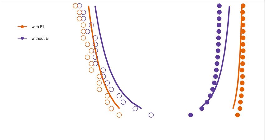
Figure 7 shows the nC comparison for a sensitivity analysis on risk r using the three scenarios for
the dilemma with EI using heterogeneous income loss (i.e., running the agent-based simulations).
In order to get the lines of the plot we averaged a sufficient set of values for initial frequency of
cooperators n0C by following each of the three scenarios. The set of values is from n0C = 0 to
n0C = 0.5 as policies should be focus on a reduced number of players in the population and it is
not suitable for the comparison to restrict initial cooperators to a high number.
The results of the plot are clear. When the system starts with those players having the lowest
income loss as cooperators, the final cooperation of the population increases significantly. On the
opposite, when we fix the initial cooperators to those having the highest income loss, the final co-
operation even decreases with respect to the random initial cooperators setting. Final cooperation
increase of negative bias with respect to positive bias is between 10% and 50% depending on the
risk values. Just when risk values are below 0.1, all the scenarios have equal results as the dilemma
does not facilitate any final cooperation.
4. Conclusions
COVID-19 pandemic and other global risks have changed how regions or countries interact
concerning global failures such as economic knockdowns. In these cases, there are economic inter-
15Figure 7: Comparison on different initial conditions n0C for achieving the best final frequency of cooperation nC in
the population. Initial coordination of players with the lowest income loss can drive the entire population to higher
levels of cooperation. On the opposite, if the initial cooperators face a significant income loss, cooperation tends to
decrease compared with the random case. This result shows that heterogeneity leads to different liabilities, depending
on the level of exposure. Moreover, it suggests that one may profit from heterogeneity to trigger prosociality at the
global level. Parameters: Z = 2 × 10³ , N = 10, M=7, β = 1, and µ = 1/Z.
dependences (EIs) or spillover effects among players when facing public goods games. For instance,
economic or mobility restrictions set by some players can affect the expected payoff by defecting
ones or free-riders. To cope with this new reality, we proposed a collective risk dilemma (CRD)
that includes EI effects among players. Real data from the tourism contribution of the EU regions
is employed to enrich the model by setting a genuine heterogeneous distribution of cooperation
costs for the players.
We show that EI robustly increases cooperation for both homogeneous and heterogeneous cases.
EI is able to modify the (finite population analogues of) internal fixed points when compared with
the dynamics in the absence of EI. We depart from a classic CRD characterized by defector dom-
16inance and coexistence among cooperators and defectors, each outcome associated with two well-
defined basins of attraction. In the absence of any additional community enforcement mechanism,
EI drops the minimum number of cooperators required to reach the cooperative basin of attraction,
and increase the prevalence of cooperators in coexistence point. We have computed these fixed
points analytically for scenarios with homogeneous costs and through agent-based simulations in
the case of heterogeneous costs. To this end, in the latter, we proposed a new method to infer
these finite population analogues of stable and unstable fixed points in infinite populations from
the simulation’s outputs.
Finally, we have discussed how biased initial conditions based on the level of exposure may
alter the final expected outcome. Results showed that the entire population benefits from having
cooperators within the sub-group of players with lower income loss. This result suggests that one
may profit from heterogeneity in designing effective interventions or governance policies to trigger
prosociality at the global level, a result of particular importance if we consider that individual
strategies may also depend on the perceived risk by each party [3]. Interventions should focus on
those players showing a lower exposure to the economic risk.
Future work can assess if rewarding and sanctioning activities can be applied [41, 6, 14, 8,
40, 18] to a specific target sub-population and the features of this subset of individuals to target,
or how positive, and negative incentives can be optimally distributed among groups and actors.
Moreover, reactions to the COVID-19 pandemic have shown a wide range of (often polarized)
responses. Recent results have shown how uncertainty may influence how each individual perceives
the dilemma [9, 37, 11, 5], potentially leading to polarized reactions [10], a development yet to be
studied in the context of cooperation dynamics related to managing economic losses under pandemic
conditions. Finally, how leaders act and influence others by their example and reputation can affect
the whole population outcome [43], and this phenomenon can be studied for this dilemma. All
these open questions remain critical in the current quest of understanding and promoting human
cooperation, given the difficulty in assessing the advantages and disadvantages of each possible
type of intervention policies.
17Acknowledgments
M.C. is supported by the Spanish Ministry of Science, Andalusian Government, and ERDF un-
der grants SIMARK (P18-TP-4475), RYC-2016-19800, and Jose Castillejo program (CAS19/00090).
J.M.H. is supported by the University of Las Palmas de Gran Canaria under grant COVID-19 04.
F.C.S. acknowledges the support from FCT-Portugal (grants UIDB/50021/2020, PTDC/MAT-
APL/6804/2020, and PTDC/CCI-INF/7366/2020).
References
[1] Abou Chakra, M., Traulsen, A., 2012. Evolutionary Dynamics of Strategic Behavior in a Collective-Risk
Dilemma. PLoS Computational Biology 8, 1–7.
[2] Adami, C., Schossau, J., Hintze, A., 2016. Evolutionary game theory using agent-based methods. Physics of
life reviews 19, 1–26.
[3] Amaral, M.A., de Oliveira, M.M., Javarone, M.A., 2021. An epidemiological model with voluntary quarantine
strategies governed by evolutionary game dynamics. Chaos, Solitons & Fractals 143, 110616.
[4] Bank, W., 2020. Gdp growth. URL: https://data.worldbank.org/indicator/NY.GDP.MKTP.KD.ZG.
[5] Barfuss, W., Donges, J.F., Vasconcelos, V.V., Kurths, J., Levin, S.A., 2020. Caring for the future can turn
tragedy into comedy for long-term collective action under risk of collapse. Proc Natl Acad Sci USA 117,
12915–12922.
[6] Chen, X., Sasaki, T., Brännström, Å., Dieckmann, U., 2015. First carrot, then stick: how the adaptive hy-
bridization of incentives promotes cooperation. Journal of the royal society interface 12, 20140935.
[7] Chica, M., Hernández, J.M., Bulchand-Gidumal, J., 2021. A collective risk dilemma for tourism restrictions
under the COVID-19 context. Scientific Reports 11, 1–12.
[8] Couto, M.C., Pacheco, J.M., Santos, F.C., 2020. Governance of risky public goods under graduated punishment.
Journal of Theoretical Biology 505, 110423.
[9] Dannenberg, A., Löschel, A., Paolacci, G., Reif, C., Tavoni, A., 2015. On the provision of public goods with
probabilistic and ambiguous thresholds. Environmental and Resource economics 61, 365–383.
[10] Domingos, E.F., Grujić, J., Burguillo, J.C., Kirchsteiger, G., Santos, F.C., Lenaerts, T., 2020. Timing uncer-
tainty in collective risk dilemmas encourages group reciprocation and polarization. iScience 23, 101752.
[11] Domingos, E.F., Grujić, J., Burguillo, J.C., Santos, F.C., Lenaerts, T., 2021. Modeling behavioral experiments
on uncertainty and cooperation with population-based reinforcement learning. Simulation Modelling Practice
and Theory 109, 102299.
[12] Eurostat, 2020. Nights spent at tourist accommodation establishments by nuts 2 regions. https://ec.europa.
eu/eurostat/web/products-datasets/-/tgs00111. Accessed: 2021-01-21.
[13] Fernandes, N., 2020. conomic effects of coronavirus outbreak (covid-19) on the world economy. SSRN Electronic
Journal, ISSN 1556-5068, Elsevier BV, , 0–29.
18[14] Góis, A.R., Santos, F.P., Pacheco, J.M., Santos, F.C., 2019. Reward and punishment in climate change dilemmas.
Scientific Reports 9, 1–9.
[15] Hauert, C., Michor, F., Nowak, M.A., Doebeli, M., 2006. Synergy and discounting of cooperation in social
dilemmas. Journal of theoretical biology 239, 195–202.
[16] Hofbauer, J., Sigmund, K., et al., 1998. Evolutionary games and population dynamics. Cambridge university
press.
[17] Holtz, D., Zhao, M., Benzell, S.G., Cao, C.Y., Rahimian, M.A., Yang, J., Allen, J., Collis, A., Moehring, A.,
Sowrirajan, T., Ghosh, D., Zhang, Y., Dhillon, P.S., Nicolaides, C., Eckles, D., Aral, S., 2020. Interdependence
and the cost of uncoordinated responses to COVID-19. Proceedings of the National Academy of Sciences of the
United States of America 117, 19837–19843.
[18] Hu, L., He, N., Weng, Q., Chen, X., Perc, M., 2020. Rewarding endowments lead to a win-win in the evolution
of public cooperation and the accumulation of common resources. Chaos, Solitons & Fractals 134, 109694.
[19] Li, X., Hao, G., Zhang, Z., Xia, C., 2021. Evolution of cooperation in heterogeneously stochastic interactions.
Chaos, Solitons & Fractals 150, 111186.
[20] Macal, C.M., North, M.J., 2005. Tutorial on agent-based modeling and simulation, in: Proceedings of the 37th
conference on Winter simulation, ACM. pp. 2–15.
[21] Milinski, M., Röhl, T., Marotzke, J., 2011. Cooperative interaction of rich and poor can be catalyzed by
intermediate climate targets. Climatic change 109, 807–814.
[22] Milinski, M., Sommerfeld, R.D., Krambeck, H.J., Reed, F.A., Marotzke, J., 2008. The collective-risk social
dilemma and the prevention of simulated dangerous climate change. Proc Natl Acad Sci USA 105, 2291–2294.
[23] Nowak, M.A., 2006. Evolutionary dynamics: exploring the equations of life. Harvard university press.
[24] Nowak, M.A., Sasaki, A., Taylor, C., Fudenberg, D., 2004. Emergence of cooperation and evolutionary stability
in finite populations. Nature 428, 646–650.
[25] Ozili, P.K., Arun, T., 2020. Spillover of COVID-19: Impact on the Global Economy. SSRN Electronic Journal
99850.
[26] Pacheco, J.M., Santos, F.C., Souza, M.O., Skyrms, B., 2009. Evolutionary dynamics of collective action in
n-person stag hunt dilemmas. Proceedings of the Royal Society B: Biological Sciences 276, 315–321.
[27] Pacheco, J.M., Vasconcelos, V.V., Santos, F.C., 2014. Climate change governance, cooperation and self-
organization. Physics of Life Reviews 11, 573–586.
[28] Pahl, S., Brandi, C., Schwab, J., Stender, F., 2021. Cling together, swing together: The contagious effects of
COVID-19 on developing countries through global value chains. World Economy , 1–22.
[29] Perc, M., Jordan, J.J., Rand, D.G., Wang, Z., Boccaletti, S., Szolnoki, A., 2017. Statistical physics of human
cooperation. Physics Reports 687, 1–51.
[30] Perc, M., Szolnoki, A., 2010. Coevolutionary games—a mini review. BioSystems 99, 109–125.
[31] Pham, T.D., Dwyer, L., Su, J.J., Ngo, T., 2021. COVID-19 impacts of inbound tourism on Australian economy.
Annals of Tourism Research 88, 103179.
[32] Pinheiro, F.L., Santos, F.C., Pacheco, J.M., 2016. Linking individual and collective behavior in adaptive social
networks. Physical Review Letters 116, 128702.
19[33] Santos, F.C., Pacheco, J.M., 2011. Risk of collective failure provides an escape from the tragedy of the commons.
Proceedings of the National Academy of Sciences 108, 10421–10425.
[34] Sigmund, K., 2010. The calculus of selfishness. Princeton University Press.
[35] Svoboda, J., Tkadlec, J., Pavlogiannis, A., Chatterjee, K., Nowak, M.A., 2020. Infection dynamics of covid-19
virus under lockdown and reopening .
[36] Szabó, G., Tőke, C., 1998. Evolutionary prisoner’s dilemma game on a square lattice. Physical Review E 58,
69.
[37] Tavoni, A., Dannenberg, A., Kallis, G., Löschel, A., 2011. Inequality, communication, and the avoidance of
disastrous climate change in a public goods game. Proc Natl Acad Sci USA 108, 11825–11829.
[38] Traulsen, A., Nowak, M.A., Pacheco, J.M., 2006a. Stochastic dynamics of invasion and fixation. Physical Review
E 74, 011909.
[39] Traulsen, A., Nowak, M.A., Pacheco, J.M., 2006b. Stochastic dynamics of invasion and fixation. Physical
Review E - Statistical, Nonlinear, and Soft Matter Physics 74, 1–10.
[40] Vasconcelos, V.V., Hannam, P.M., Levin, S.A., Pacheco, J.M., 2020. Coalition-structured governance improves
cooperation to provide public goods. Scientific reports 10, 1–10.
[41] Vasconcelos, V.V., Santos, F.C., Pacheco, J.M., 2013. A bottom-up institutional approach to cooperative
governance of risky commons. Nature Climate Change 3, 797.
[42] Vasconcelos, V.V., Santos, F.C., Pacheco, J.M., Levin, S.A., 2014. Climate policies under wealth inequality.
Proceedings of the National Academy of Sciences of the United States of America 111, 2212–2216.
[43] Wang, Z., Chen, T., Wang, Y., 2017. Leadership by example promotes the emergence of cooperation in public
goods game. Chaos, Solitons & Fractals 101, 100–105.
20You can also read