COVID-19 Healthcare Demand Projections: Houston-The Woodlands-Sugar Land MSA, Texas

COVID-19 Healthcare Demand
Projections: Houston-The
Woodlands-Sugar Land MSA, Texas

Kelly Pierce, Ethan Ho, Xutong Wang, Remy Pasco, Zhanwei Du,
Spencer Fox, Greg Zynda, Jawon Song, Lauren Ancel Meyers

The University of Texas at Austin
COVID-19 Modeling Consortium
utpandemics@austin.utexas.edu

COVID-19 Healthcare Demand
Projections: Houston-The
Woodlands-Sugar Land MSA, Texas
The University of Texas COVID-19 Modeling Consortium
Contributors: Kelly Pierce, Ethan Ho, Xutong Wang, Remy Pasco, Zhanwei Du,
Spencer Fox, Greg Zynda, Jawon Song, Lauren Ancel Meyers
Contact: utpandemics@austin.utexas.edu

Overview
To support healthcare planning, we analyzed the Houston-The Woodlands-Sugar Land
MSA module of our ​US COVID-19 Pandemic Model​ to project the number of cases,
healthcare requirements and deaths under different scenarios. Note that the results
presented herein are based on multiple assumptions about the transmission rate and
age-specific severity of COVID-19. There is still much we do not understand about the
transmission dynamics of this virus, including the extent of asymptomatic infection and
transmission. These results do not represent the full range of uncertainty. Rather, they
are meant to serve as plausible scenarios for gauging the likely impacts of control
measures in the Houston-The Woodlands-Sugar Land MSA.

We have updated our model inputs based on the daily number of COVID-19
hospitalizations in Houston-The Woodlands-Sugar Land between April 2, 2020 and April
20, 2020, provided by the Southeast Texas Regional Advisory Council (SETRAC). The
projections assume that schools were closed on March 19, 2020 (start of state
mandated school closures) and extensive social distancing began on March 24, 2020
with Houston and Harris County’s Stay Home Work Safe order ​[1]​. The data suggest
that recent social distancing has reduced transmission by anywhere between 80% and
100% relative to the period prior to March 19th. We make projections for five different
scenarios. The first three–80%, 95% and 100% reductions in transmission–fall within
this range of current estimates; the other two–0% and 50% reductions in
transmission–provide more pessimistic projections that could occur with extreme
relaxation of social distancing measures. For each of the scenarios, the graphs project
COVID-19 cases, hospitalizations, patients requiring ICU care, patients requiring
ventilation and deaths.

UT COVID-19 Consortium 1 April 28, 2020

We are posting these results prior to peer review to provide intuition for both policy
makers and the public regarding both the immediate threat of COVID-19 and the extent
to which continued social distancing, transmission-reducing precautions such as
keeping physical distance and wearing cloth face coverings, can mitigate that threat.

COVID-19 projections for Houston-The
Woodlands-Sugar Land MSA
We updated the Houston-The Woodlands-Sugar Land MSA module of our US
COVID-19 Pandemic Model to simulate COVID-19 epidemics under various
assumptions about the efficacy of social distancing measures.

Hospitalization data from the Houston-The Woodlands-Sugar Land MSA suggest that
the ongoing COVID-19 epidemic was likely seeded in early February. The simulations
thus assume the epidemic began with a single infected adult on February 10, 2020 and
project transmission for 175 days through mid-August based on the following
assumptions:

 ● Starting deterministic condition: February 10, 2020 with 1 infected adult

 ● Starting stochastic condition: at least 10 symptomatic cases total. For the
 Houston-The Woodlands-Sugar Land model this threshold is met on February
 23, 2020.

 ● Time course of interventions

 ○ February 10 - March 18, 2020: No interventions

 ○ March 19 - August 16, 2020: Schools closed

 ○ March 24 - August 16, 2020: social distancing intervention reduces
 transmission (beyond school closures) by an additional 50%, 80%, 95%
 and 100%

 ● β = 0.035 (based on fitting our model to daily COVID-19 hospitalizations in Austin
 Round-Rock MSA for March 13-April 24, 2020). This corresponds to an epidemic
 doubling time of 2.9 days prior to March 19, 2020.

 ● Average incubation period (assuming 12.1% of transmission happens
 pre-symptomatically): 6.9 days ​[2]

UT COVID-19 Consortium 2 April 28, 2020

● Proportion of cases asymptomatic (assumed 46% as infectious as symptomatic
 cases): 17.9% ​[3]

Table 1 and Figures 1-5 summarize results of COVID-19 simulations for the
Houston-The Woodlands-Sugar Land MSA. Each stochastic simulation began on
February 23, 2020 with approximately 10 infectious COVID-19 cases and ended on
August 16, 2020. The model structure and parameters, including age-specific
hospitalization and fatality rates, are described in the Appendices below.

Table 1. Estimated cumulative COVID-19 cases, hospitalizations, ICU cases, cases requiring
mechanical ventilatory therapy, and deaths for the Houston-The Woodlands-Sugar Land MSA
from February 23, 2020 to August 16 2020.​ The values are medians (with full range in
parentheses) across 300 stochastic simulations based on the parameters given in Appendix 1.

 Outcomes (Cumulative February 23 - August 16, 2020)
 Contact
reduction Cases Hospitalizations ICU beds Ventilators Deaths

 School 5,734,903 312,253 37,425 17,822 38,786
 closure (5,732,110- (311,283- (37,313-37,605) (17,768-17,907) (38,136-39,288)
 only 5,737,977) 313,606)

 5,492,249 285,971 34,355 16,360 33,393
 50% (5,363,306- (271,713-294,474) (3,2646-35,373) (15,546-16,844) (30,684-35,202)
 5,560,703)
 1,175,502
 45,247 5,467 2,604 4,154
 80% (551,894-
 (20,543-103,154) (2,478-12,450) (1,180-5,929) (1,856-10,125)
 2,426,190)

 76,918 3,554
 95% 430 (214-1,096) 205 (102-522) 355 (168-874)
 (37,818-196,765) (1,759-9,054)

 50,099
 100% 2,299 (859-6,291) 278 (104-759) 133 (50-362) 225 (92-615)
 (18,193-135,650)

UT COVID-19 Consortium 3 April 28, 2020

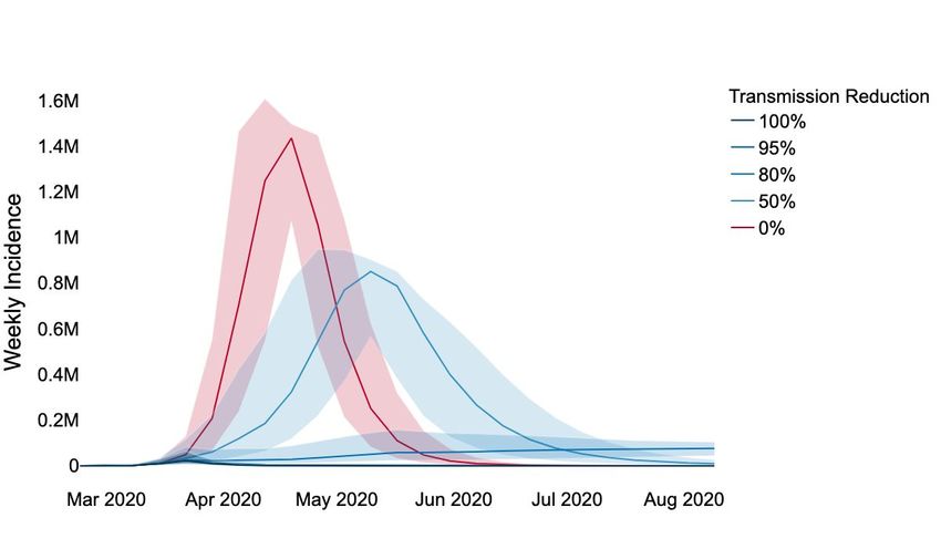
Figure 1. Projected COVID-19 cases in the Houston-The Woodlands-Sugar Land MSA from
February 23, 2020 to August 16, 2020 coupled with different degrees of social distancing
starting March 24, 2020.​ The red line projects COVID-19 transmission assuming that there was no
reduction in transmission from social distancing beyond a modest effect of school closures. The blue
lines show increasing levels of social distancing efficacy, from light to dark: 50%, 80%, 95%, and
100% reductions in transmission. Lines and shading indicate the minimum, median and maximum
values across 300 stochastic simulations.

UT COVID-19 Consortium 4 April 28, 2020

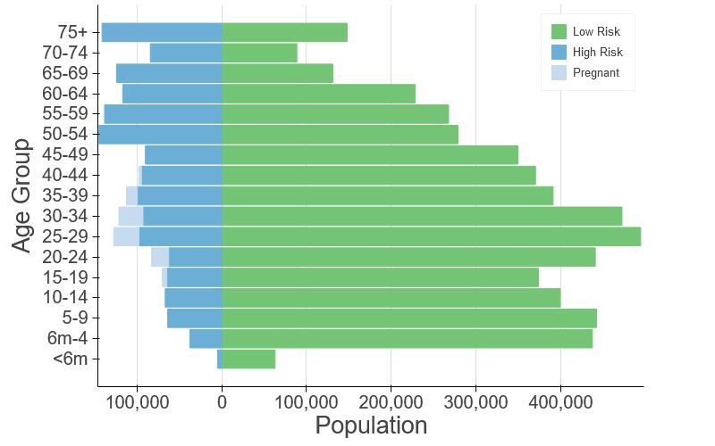
Figure 2. Projected daily COVID-19 hospitalizations in Houston-The Woodlands-Sugar Land
MSA from February 23, 2020 to August 16, 2020 coupled with different degrees of social
distancing starting March 24, 2020.​ The two graphs are identical except that the top graph only
shows hospitalizations up to 1000 per day and includes the reported total daily COVID-19
hospitalizations across all reporting Houston-The Woodlands-Sugar Land MSA hospitals (black
points). In both graphs, the red lines project COVID-19 hospitalizations assuming that there was no
reduction in transmission from social distancing beyond a modest effect of school closures. The blue
lines show increasing levels of social distancing efficacy, from light to dark: 50%, 80%, 95%, and
100% reductions in transmission. Lines and shading indicate the minimum, median and maximum
values across 300 stochastic simulations.

UT COVID-19 Consortium 5 April 28, 2020

Figure 3. Projected COVID-19 cases requiring ICU treatment in Houston-The
Woodlands-Sugar Land MSA from February 23, 2020 to August 16, 2020 coupled with
different degrees of social distancing starting March 24, 2020.​ The red line projects COVID-19
ICU patients assuming that there was no reduction in transmission from social distancing beyond a
modest effect of school closures. The blue lines show increasing levels of social distancing efficacy,
from light to dark: 50%, 80%, 95%, and 100% reductions in transmission. Lines and shading indicate
the minimum, median and maximum values across 300 stochastic simulations.

UT COVID-19 Consortium 6 April 28, 2020

Figure 4. Projected COVID-19 cases requiring mechanical ventilation in Houston-The
Woodlands-Sugar Land MSA from February 23, 2020 to August 16, 2020 coupled with
different degrees of social distancing starting March 24, 2020.​ The red line projects ventilated
COVID-19 patients assuming that there was no reduction in transmission from social distancing
beyond a modest effect of school closures. The blue lines show increasing levels of social distancing
efficacy, from light to dark: 50%, 80%, 95%, and 100% reductions in transmission. Lines and
shading indicate the minimum, median and maximum values across 300 stochastic simulations.

UT COVID-19 Consortium 7 April 28, 2020

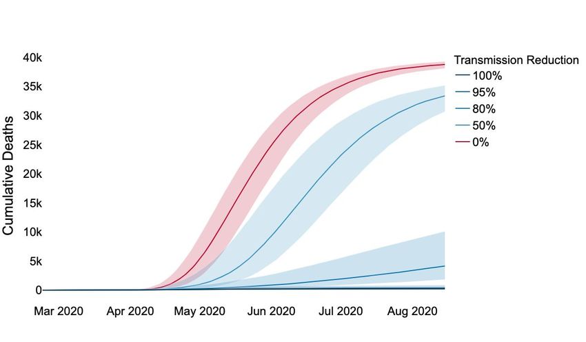
Figure 5. Projected cumulative COVID-19 deaths in Houston-The Woodlands-Sugar Land MSA
from February 23, 2020 to August 16, 2020 coupled with different degrees of social distancing
starting March 24, 2020.​ The red line projects cumulative COVID-19 deaths assuming that there
was no reduction in transmission from social distancing beyond a modest effect of school closures.
The blue lines show increasing levels of social distancing efficacy, from light to dark: 50%, 80%,
95%, and 100% reductions in transmission. Lines and shading indicate the minimum, median and
maximum values across 300 stochastic simulations.

Appendix

COVID-19 Epidemic Model Structure and Parameters
The model structure is diagrammed in Figure A1 and described in the equations below.
For each age and risk group, we build a separate set of compartments to model the transitions
between the states: susceptible (S), exposed (E), symptomatic infectious (I​Y​), asymptomatic
infectious (I​A​), symptomatic infectious that are hospitalized (I​H​), recovered (R), and deceased
(D). The symbols S, E, I​Y​, I​A​, I​H​, R, and D denote the number of people in that state in the given
age/risk group and the total size of the age/risk group is .
The model for individuals in age group and risk group is given by:

UT COVID-19 Consortium 8 April 28, 2020

A Y H
where A and K are all possible age and risk groups, , , are relative infectiousness of the
I A , I Y , E compartments, respectively, is transmission rate, a,i is the mixing rate between age
 A Y H
group a, i ∈ A , , , are the recovery rates for the I A , I Y , I H compartments, respectively, 
is the exposed rate, is the symptomatic ratio, is the proportion of symptomatic individuals
requiring hospitalization, is rate at which hospitalized cases enter the hospital following
symptom onset, is mortality rate for hospitalized cases, and is rate at which terminal patients
die.

We simulate the model using a hybrid approach combining a deterministic initial phase (up to 10
cumulative cases) followed by a stochastic phase implemented as follows. Transitions between
compartments are governed using the -leap method ​[4,5]​ with key parameters given in Table
S1. Assuming that the events at each time-step are independent and do not impact the
underlying transition rates, the numbers of each type of event should follow Poisson
distributions with means equal to the rate parameters. We thus simulate the model according to
the following equations:

 ,

 with

UT COVID-19 Consortium 9 April 28, 2020

and where denotes the force of infection for individuals in age group and risk group
and is given by:

Figure A1. Compartmental model of COVID-19 transmission in a US city. ​Each subgroup (defined by
age and risk) is modeled with a separate set of compartments. Upon infection, susceptible individuals (S)
progress to exposed (E) and then to either symptomatic infectious (I​Y​) or asymptomatic infectious (I​A​). All
asymptomatic cases eventually progress to a recovered class where they remain protected from future
infection (R); symptomatic cases are either hospitalized (I​H​) or recover. Mortality (D) varies by age group
and risk group and is assumed to be preceded by hospitalization.

Estimating the effect of the Stay Home-Work Safe order
We estimated the transmission rate of COVID-19 in the Houston-The Woodlands-Sugar Land
MSA before and after the March 24th Stay at Home order using least-squares fitting, which
compares the predicted and observed numbers of daily hospitalizations (i.e., heads in beds) for
the Houston-The Woodlands-Sugar Land MSA. We assume that: (i) the epidemic starts with an
initial transmission rate of = 0.035, (ii) the transmission rate decreases when school closures
are enacted on March 19, 2020 (by an amount determined by our pre-set contact matrices), (iii)
the transmission rate decreases further by an amount on March 24th following the ​Stay
Home-Work Safe​ order.

UT COVID-19 Consortium 10 April 28, 2020

We estimate using a nonlinear least squares fitting procedure in the SciPy/Python package
across a range of possible start dates ​[6]​. For a given start date, we run a deterministic
simulation of our model assuming a central value for . Using a trust region method, the
algorithm finds value of that minimize the sum of squared daily differences between the
simulated ( ) and actual ( ) daily hospitalizations from April 2, 2020 through April 20, 2020:

for the assumed start date as . We then select the start date that
produces the lowest normalized mean square deviation and fix that start date for subsequent
simulations. For the Houston-The Woodlands-Sugar Land MSA, the best-fit start date is
February 10, 2020.

We calculated 95% confidence intervals for the social distancing parameter indirectly by
running 500 stochastic simulations for each of the following possible values of : 0.0, 0.05, ....,
0.95, 1.0. For each value of , we conducted the following analysis to determine if lies inside
the 95% confidence interval for .

 ● For all simulations, we calculate the day-to-day difference in hospitalizations (i.e., heads
 in beds) during the period following the ​Stay Home-Work Safe​ order: .
 We do the same for the actual data: .

 ● We compute the 95% prediction interval for across all 500 stochastic simulations for
 for each day .

 ● We then conduct a test of the null hypothesis . Under this null hypothesis,
 we would expect roughly 95% of the observed data ( ) to fall within the 95% prediction
 band for that we constructed from our simulations. By analyzing the day-to-day
 difference in hospitalizations rather than daily hospitalizations, we can assume that the
 data are independent from one day to the next. Then the expected number of observed
 values contained in the 95% prediction band is given by the binomial expression:

 where is the number of data points contained within the 95% prediction band
 and is the total number of data points (i.e., days).
 ● If the binomial probability of ​ is less than 0.05, we reject the null hypothesis

To construct a 95% confidence interval for we take the minimum and maximum for which
we did not reject the null hypothesis .

UT COVID-19 Consortium 11 April 28, 2020

Table A1. Initial conditions, school closures and social distancing policies
Variable Settings

 Initial day of simulation February 10, 2020

 Initial infection number
 1 symptomatic case in 18-49y age group
 in locations

 School closure March 19, 2020 - August 16, 2020

 Social distancing
 Five scenarios: ​[0.0, 0.5, 0.8, 0.95, 1.0]
 reduction in contacts

 Home, work, other and school matrices provided in Tables S4.1-S4.4

 ● From February 10, 2020 to March 18, 2020
 ○ Weekday = home + school + work + other
 ○ Weekend = home + other
 ○ Weekday holiday = home + other
 Age-specific and ● From March 19, 2020 to March 23, 2020
 day-specific contact ○ Weekday = home + work + other
 rates ○ Weekend = home + other
 ○ Weekday holiday = home + other
 ● From March 24, 2020
 ○ Weekday = (1-ɑ)*(home + work + other)
 ○ Weekend = (1-ɑ)*(home + other)
 ○ Weekday holiday = (1-ɑ)*(home + other)

Table A2. Model parameters​a

 Parameters Value Source

 Fitted to daily COVID-19
 : transmission rate 0.035 hospitalizations in Austin-Round
 Rock MSA

 : recovery rate on
 asymptomatic Equal to
 compartment

 : recovery rate on
 symptomatic non-treated Verity et al. ​[7]
 compartment

 : symptomatic
 82.1 Mizumoto et al. ​[3]
 proportion (%)

UT COVID-19 Consortium 12 April 28, 2020

: exposed rate Lauer et al. ​[2]

 ​P:​ proportion of
 pre-symptomatic 12.6 Du et al. ​[8]
 transmission (%)

 : relative
 infectiousness of
 infectious individuals in
 compartment E

 : relative
 infectiousness of
 0.4653 Set to mean of
 infectious individuals in
 compartment I​A

 Low risk: [0.0009, 0.0022, 0.0339,
 IFR:​ infected fatality 0.2520, 0.6440]
 Age adjusted from Verity et al. ​[7]
 ratio, age specific (%) High risk: [0.0092, 0.0218, 0.3388,
 2.5197, 6.4402]

 Low risk: [0.0011165, 0.0027 ,
 YFR:​ symptomatic
 0.0412, 0.3069, 0.7844]
 fatality ratio, age specific
 High risk: [0.0112, 0.0265, 0.4126,
 (%)
 3.0690, 7.8443]

 Estimated using 2015-2016
 Behavioral Risk Factor Surveillance
 System (BRFSS) data with
 h : high-risk proportion, [8.2825, 14.1121, 16.5298, multilevel regression and
 age specific (%) 32.9912, 47.0568] poststratification using CDC’s list of
 conditions that may increase the
 risk of serious complications from
 influenza ​[9–11]

a​
 Values given as five-element vectors are age-stratified with values corresponding to 0-4, 5-17, 18-49,
50-64, 65+ year age groups, respectively.

UT COVID-19 Consortium 13 April 28, 2020

Table A3 Hospitalization parameters

 Parameters Value Source

 : recovery rate in 14 day-average from admission
 hospitalized 1/14 to discharge (UT Austin Dell
 compartment Med)

 Low risk: [0.0279, 0.0215, 1.3215,
 YHR:​ symptomatic
 2.8563, 3.3873] Age adjusted from Verity et al.
 case hospitalization
 High risk: [ 0.2791, 0.2146, 13.2154, [7]
 rate (%)
 28.5634, 33.8733]

 : rate of symptomatic
 individuals go to
 hospital, age-specific

 5.9 day average from symptom
 : rate from symptom
 0.1695 onset to hospital admission
 onset to hospitalized
 Tindale et al.​[12]

 : rate from 14 day-average from admission
 1/14
 hospitalized to death to death (UT Austin Dell Med)

 HFR​: hospitalized
 fatality ratio, age [4, 12.365, 3.122, 10.745, 23.158]
 specific (%)

 : death rate on
 hospitalized
 [0.0390, 0.1208, 0.0304, 0.1049, 0.2269]
 individuals, age
 specific

 ICU:​ proportion CDC planning scenarios
 hospitalized people in [0.15, 0.20, 0.15, 0.20, 0.15] (based on US seasonal flu
 ICU data)

 Vent:​ proportion of
 individuals in ICU 0.67 Assumption
 needing ventilation

 dICU : duration of stay Assumption, set equal to
 10 days
 in ICU duration of ventilation

 dV : duration of
 10 days Assumption
 ventilation

UT COVID-19 Consortium 14 April 28, 2020

Table A4.1 Home contact matrix. ​Daily number contacts by age group at home.
 0-4y 5-17y 18-49y 50-64y 65y+

 0-4y 0.5 0.9 2.0 0.1 0.0

 5-17y 0.2 1.7 1.9 0.2 0.0

 18-49y 0.2 0.9 1.7 0.2 0.0

 50-64y 0.2 0.7 1.2 1.0 0.1

 65y+ 0.1 0.7 1.0 0.3 0.6

Table A4.2 School contact matrix. ​Daily number contacts by age group at school.
 0-4y 5-17y 18-49y 50-64y 65y+

 0-4y 1.0 0.5 0.4 0.1 0.0

 5-17y 0.2 3.7 0.9 0.1 0.0

 18-49y 0.0 0.7 0.8 0.0 0.0

 50-64y 0.1 0.8 0.5 0.1 0.0

 65y+ 0.0 0.0 0.1 0.0 0.0

Table A4.3 Work contact matrix. ​Daily number contacts by age group at work.
 0-4y 5-17y 18-49y 50-64y 65y+

 0-4y 0.0 0.0 0.0 0.0 0.0

 5-17y 0.0 0.1 0.4 0.0 0.0

 18-49y 0.0 0.2 4.5 0.8 0.0

 50-64y 0.0 0.1 2.8 0.9 0.0

 65y+ 0.0 0.0 0.1 0.0 0.0

Table A4.4 Others contact matrix. ​Daily number contacts by age group at other locations.
 0-4y 5-17y 18-49y 50-64y 65y+

 0-4y 0.7 0.7 1.8 0.6 0.3

 5-17y 0.2 2.6 2.1 0.4 0.2

 18-49y 0.1 0.7 3.3 0.6 0.2

 50-64y 0.1 0.3 2.2 1.1 0.4

 65y+ 0.0 0.2 1.3 0.8 0.6

UT COVID-19 Consortium 15 April 28, 2020

Estimation of age-stratified proportion of population at high-risk for
COVID-10 complications
We estimate age-specific proportions of the population at high risk of complications from
COVID-19 based on data for the Houston-The Woodlands-Sugar Land MSA from the CDC’s
500 cities project (Figure A2) ​[13]​. We assume that high risk conditions for COVID-19 are the
same as those specified for influenza by the CDC ​[9]​. The CDC’s 500 cities project provides
city-specific estimates of prevalence for several of these conditions among adults ​[14]​. The
estimates were obtained from the 2015-2016 Behavioral Risk Factor Surveillance System
(BRFSS) data using a small-area estimation methodology called multi-level regression and
poststratification ​[10,11]​. It links geocoded health surveys to high spatial resolution population
demographic and socioeconomic data ​[11]​.

Estimating high-risk proportions for adults. ​To estimate the proportion of adults at high risk
for complications, we use the CDC’s 500 cities data, as well as data on the prevalence of
HIV/AIDS, obesity and pregnancy among adults (Table A6).

The CDC 500 cities dataset includes the prevalence of each condition on its own, rather than
the prevalence of multiple conditions (e.g., dyads or triads). Thus, we use separate co-morbidity
estimates to determine overlap. Reference about chronic conditions ​[15]​ gives US estimates for
the proportion of the adult population with 0, 1 or 2+ chronic conditions, per age group. Using
this and the 500 cities data we can estimate the proportion of the population pHR in each age
group in each city with at least one chronic condition listed in the CDC 500 cities data (Table
A6) putting them at high-risk for flu complications.

HIV​: We use the data from table 20a in CDC HIV surveillance report ​[16]​ to estimate the
population in each risk group living with HIV in the US (last column, 2015 data). Assuming
independence between HIV and other chronic conditions, we increase the proportion of the
population at high-risk for influenza to account for individuals with HIV but no other underlying
conditions.

Morbid obesity​: A BMI over 40kg/m​2 ​indicates morbid obesity, and is considered high risk for
influenza. The 500 Cities Project reports the prevalence of obese people in each city with BMI
over 30kg/m​2​ (not necessarily morbid obesity). We use the data from table 1 in Sturm and
Hattori ​[17]​ to estimate the proportion of people with BMI>30 that actually have BMI>40 (across
the US); we then apply this to the 500 Cities obesity data to estimate the proportion of people
who are morbidly obese in each city. Table 1 of Morgan et al. ​[18]​ suggests that 51.2% of
morbidly obese adults have at least one other high risk chronic condition, and update our
high-risk population estimates accordingly to account for overlap.

UT COVID-19 Consortium 16 April 28, 2020

Pregnancy​: We separately estimate the number of pregnant women in each age group and
each city, following the methodology in CDC reproductive health report ​[19]​. We assume
independence between any of the high-risk factors and pregnancy, and further assume that half
the population are women.

Estimating high-risk proportions for children.​ Since the 500 Cities Project only reports data
for adults 18 years and older, we take a different approach to estimating the proportion of
children at high risk for severe influenza. The two most prevalent risk factors for children are
asthma and obesity; we also account for childhood diabetes, HIV and cancer.
From Miller et al. ​[20]​, we obtain national estimates of chronic conditions in children. For
asthma, we assume that variation among cities will be similar for children and adults. Thus, we
use the relative prevalences of asthma in adults to scale our estimates for children in each city.
The prevalence of HIV and cancer in children are taken from CDC HIV surveillance report ​[16]
and cancer research report ​[21]​, respectively.

We first estimate the proportion of children having either asthma, diabetes, cancer or HIV
(assuming no overlap in these conditions). We estimate city-level morbid obesity in children
using the estimated morbid obesity in adults multiplied by a national constant ratio for each age
group estimated from Hales et al. ​[22]​, this ratio represents the prevalence in morbid obesity in
children given the one observed in adults. From Morgan et al. ​[18]​, we estimate that 25% of
morbidly obese children have another high-risk condition and adjust our final estimates
accordingly.

Resulting estimates.​ We compare our estimates for the Houston-The Woodlands-Sugar Land
MSA to published national-level estimates ​[23]​ of the proportion of each age group with
underlying high risk conditions (Table A7). We estimate a higher proportion of individuals at
high-risk for complications for COVID-19 compared to the national average in almost every age
group, with the biggest difference observed in 10-19y and 35-64y groups.

UT COVID-19 Consortium 17 April 28, 2020

Figure A2. Demographic and risk composition of the Houston-The Woodlands-Sugar Land
MSA.​ ​Bars indicate age-specific population sizes, separated by low risk, high risk, and pregnant.
High risk is defined as individuals with cancer, chronic kidney disease, COPD, heart disease,
stroke, asthma, diabetes, HIV/AIDS, and morbid obesity, as estimated from the CDC 500 Cities
Project ​[13]​, reported HIV prevalence ​[16]​ and reported morbid obesity prevalence ​[17,18]​,
corrected for multiple conditions. The population of pregnant women is derived using the CDC’s
method combining fertility, abortion and fetal loss rates ​[24–26]​.

Table A6. High-risk conditions for influenza and data sources for prevalence estimation
 Condition Data source
 Cancer (except skin),
 chronic kidney disease,
 COPD, coronary heart CDC 500 cities ​[13]
 disease, stroke, asthma,
 diabetes
 HIV/AIDS CDC HIV Surveillance report ​[16]
 Obesity CDC 500 cities ​[13]​, Sturm and Hattori ​[17]​, Morgan et al. ​[18]
 Pregnancy National Vital Statistics Reports ​[24]​ and abortion data ​[25]

UT COVID-19 Consortium 18 April 28, 2020

Table A7. Comparison between published national estimates and Houston-The
Woodlands-Sugar Land MSA estimates of the percent of the population at high-risk of
influenza/COVID-19 complications.
 Houston Pregnant women
 National estimates
 Age Group (excluding (proportion of age
 [22]
 pregnancy) group)
 0 to 6 months NA 7.1 -
 6 months to 4 years 6.8 7.9 -
 5 to 9 years 11.7 12.6 -
 10 to 14 years 11.7 14.3 -
 15 to 19 years 11.8 14.6 2.5
 20 to 24 years 12.4 11.9 7.9
 25 to 34 years 15.7 15.7 9.8
 35 to 39 years 15.7 19.8 5.2
 40 to 44 years 15.7 20.2 1.2
 45 to 49 years 15.7 20.5 -
 50 to 54 years 30.6 34.1 -
 55 to 60 years 30.6 34.0 -
 60 to 64 years 30.6 33.8 -
 65 to 69 years 47.0 48.6 -
 70 to 74 years 47.0 48.7 -
 75 years and older 47.0 48.8 -

UT COVID-19 Consortium 19 April 28, 2020

References
1. Ready Harris > Stay Home. [cited 27 Apr 2020]. Available:
 https://www.readyharris.org/Stay-Home

2. Lauer SA, Grantz KH, Bi Q, Jones FK, Zheng Q, Meredith HR, et al. The Incubation Period
 of Coronavirus Disease 2019 (COVID-19) From Publicly Reported Confirmed Cases:
 Estimation and Application. Ann Intern Med. 2020. doi:​10.7326/M20-0504

3. Mizumoto K, Kagaya K, Zarebski A, Chowell G. Estimating the Asymptomatic Proportion of
 2019 Novel Coronavirus onboard the Princess Cruises Ship, 2020. Infectious Diseases
 (except HIV/AIDS). medRxiv; 2020. doi:​10.1101/2020.02.20.20025866

4. Keeling MJ, Rohani P. Modeling Infectious Diseases in Humans and Animals. Princeton
 University Press; 2011.

5. Gillespie DT. Approximate accelerated stochastic simulation of chemically reacting
 systems. J Chem Phys. 2001;115: 1716–1733.

6. minimize(method=’trust-constr’) — SciPy v1.4.1 Reference Guide. [cited 19 Apr 2020].
 Available: ​https://docs.scipy.org/doc/scipy/reference/optimize.minimize-trustconstr.html

7. Verity R, Okell LC, Dorigatti I, Winskill P, Whittaker C, Imai N, et al. Estimates of the
 severity of COVID-19 disease. Epidemiology. medRxiv; 2020.
 doi:​10.1101/2020.03.09.20033357

8. Du Z, Xu X, Wu Y, Wang L, Cowling BJ, Meyers LA. The serial interval of COVID-19 from
 publicly reported confirmed cases. Epidemiology. medRxiv; 2020.
 doi:​10.1101/2020.02.19.20025452

9. CDC. People at High Risk of Flu. In: Centers for Disease Control and Prevention [Internet].
 1 Nov 2019 [cited 26 Mar 2020]. Available: ​https://www.cdc.gov/flu/highrisk/index.htm

10. CDC - BRFSS. 5 Nov 2019 [cited 26 Mar 2020]. Available:
 https://www.cdc.gov/brfss/index.html

11. Zhang X, Holt JB, Lu H, Wheaton AG, Ford ES, Greenlund KJ, et al. Multilevel regression
 and poststratification for small-area estimation of population health outcomes: a case study
 of chronic obstructive pulmonary disease prevalence using the behavioral risk factor
 surveillance system. Am J Epidemiol. 2014;179: 1025–1033.

12. Tindale L, Coombe M, Stockdale JE, Garlock E, Lau WYV, Saraswat M, et al. Transmission
 interval estimates suggest pre-symptomatic spread of COVID-19. Epidemiology. medRxiv;
 2020. doi:​10.1101/2020.03.03.20029983

13. 500 Cities Project: Local data for better health | Home page | CDC. 5 Dec 2019 [cited 19
 Mar 2020]. Available: ​https://www.cdc.gov/500cities/index.htm

UT COVID-19 Consortium 20 April 28, 2020

14. Health Outcomes | 500 Cities. 25 Apr 2019 [cited 28 Mar 2020]. Available:
 https://www.cdc.gov/500cities/definitions/health-outcomes.htm

15. Part One: Who Lives with Chronic Conditions. In: Pew Research Center: Internet, Science
 & Tech [Internet]. 26 Nov 2013 [cited 23 Nov 2019]. Available:
 https://www.pewresearch.org/internet/2013/11/26/part-one-who-lives-with-chronic-condition
 s/

16. for Disease Control C, Prevention, Others. HIV surveillance report. 2016; 28. URL:
 http://www cdc gov/hiv/library/reports/hiv-surveil-lance html Published November. 2017.

17. Sturm R, Hattori A. Morbid obesity rates continue to rise rapidly in the United States. Int J
 Obes . 2013;37: 889–891.

18. Morgan OW, Bramley A, Fowlkes A, Freedman DS, Taylor TH, Gargiullo P, et al. Morbid
 obesity as a risk factor for hospitalization and death due to 2009 pandemic influenza
 A(H1N1) disease. PLoS One. 2010;5: e9694.

19. Estimating the Number of Pregnant Women in a Geographic Area from CDC Division of
 Reproductive Health. Available:
 https://www.cdc.gov/reproductivehealth/emergency/pdfs/PregnacyEstimatoBrochure508.pdf

20. Miller GF, Coffield E, Leroy Z, Wallin R. Prevalence and Costs of Five Chronic Conditions in
 Children. J Sch Nurs. 2016;32: 357–364.

21. Cancer Facts & Figures 2014. [cited 30 Mar 2020]. Available:
 https://www.cancer.org/research/cancer-facts-statistics/all-cancer-facts-figures/cancer-facts
 -figures-2014.html

22. Hales CM, Fryar CD, Carroll MD, Freedman DS, Ogden CL. Trends in Obesity and Severe
 Obesity Prevalence in US Youth and Adults by Sex and Age, 2007-2008 to 2015-2016.
 JAMA. 2018;319: 1723–1725.

23. Zimmerman RK, Lauderdale DS, Tan SM, Wagener DK. Prevalence of high-risk indications
 for influenza vaccine varies by age, race, and income. Vaccine. 2010;28: 6470–6477.

24. Martin JA, Hamilton BE, Osterman MJK, Driscoll AK, Drake P. Births: Final Data for 2017.
 Natl Vital Stat Rep. 2018;67: 1–50.

25. Jatlaoui TC, Boutot ME, Mandel MG, Whiteman MK, Ti A, Petersen E, et al. Abortion
 Surveillance - United States, 2015. MMWR Surveill Summ. 2018;67: 1–45.

26. Ventura SJ, Curtin SC, Abma JC, Henshaw SK. Estimated pregnancy rates and rates of
 pregnancy outcomes for the United States, 1990-2008. Natl Vital Stat Rep. 2012;60: 1–21.

UT COVID-19 Consortium 21 April 28, 2020