Data Optimisation for a Deep Learning Recommender System
←
→
Page content transcription
If your browser does not render page correctly, please read the page content below
Data Optimisation for a Deep Learning Recommender
                                                                 System
                                                             Gustav Hertz1 , Sandhya Sachidanandan1 , Balázs Tóth1 ,
                                                                   Emil S. Jørgensen1 , and Martin Tegnér1,2
                                                 1
                                                     IKEA Group: {gustav.hertz, sandhya.sachidanandan, balazs.toth,
                                                            emil.joergensen, martin.tegner}@ingka.ikea.com
                                                                 2
                                                                   Oxford-Man Institute, University of Oxford
arXiv:2106.11218v1 [cs.IR] 21 Jun 2021

                                         Abstract                                                    making sites are common applications, to mention
                                                                                                     just but a few. Indeed, the 2012 White House report
                                         This paper advocates privacy preserving require-            on privacy and consumer data [17], and the recent
                                         ments on collection of user data for recommender            EU General Data Project Regulation in 2018, deem
                                         systems. The purpose of our study is twofold. First,        considerations of privacy and security unavoidable
                                         we ask if restrictions on data collection will hurt         for the deployer of user-centric systems.
                                         test quality of RNN-based recommendations. We                  On the other side of the coin is the fact that
                                         study how validation performance depends on the             progress in deep learning is partially enabled by
                                         available amount of training data. We use a com-            large training sets of representative data. Neural
                                         bination of top-K accuracy, catalog coverage and            networks have the potential and a proven record
                                         novelty for this purpose, since good recommenda-            of modelling input-to-output mappings with unlim-
                                         tions for the user is not necessarily captured by           ited complexity and flexibility ([11, 33, 36] are some
                                         a traditional accuracy metric. Second, we ask if            examples), but they are data greedy, especially to
                                         we can improve the quality under minimal data by            generalise well to unseen test data. “More is more”
                                         using secondary data sources. We propose knowl-             is thus the reign in the development phase of deep
                                         edge transfer for this purpose and construct a repre-       learning systems, typically on a centralised reposi-
                                         sentation to measure similarities between purchase          tory of collected data. In many applications, such
                                         behaviour in data. This to make qualified judge-            as image classification and machine translation, this
                                         ments of which source domain will contribute the            is not an issue, while interaction with users requires
                                         most. Our results show that (i) there is a saturation       care in both the collection and storage of their data.
                                         in test performance when training size is increased            This paper considers data optimisation for a
                                         above a critical point. We also discuss the interplay       deep-learning recommender system. First, we study
                                         between different performance metrics, and prop-            how the recommender system’s performance on val-
                                         erties of data. Moreover, we demonstrate that (ii)          idation data depends on the size of the training
                                         our representation is meaningful for measuring pur-         data. To this end, we use a set of performance
                                         chase behaviour. In particular, results show that we        metrics that are designed to measure the quality
                                         can leverage secondary data to improve validation           of a recommendation. This since ‘good’ recommen-
                                         performance if we select a relevant source domain           dation for the user is not necessarily represented
                                         according to our similarly measure.                         by an observable output variable; we do not have
                                                                                                     a ground-truth as our primary target,1 but rather
                                                                                                     heuristic measures for the success of a recommenda-
                                         1    Introduction                                           tion. From experiments, we conclude that there is
                                                                                                     an optimal amount of training data beyond which
                                         In the last few years, considerations of user privacy       the performance of the model either saturates or
                                         and data security have gained attention in the AI           decreases. We discuss this in terms of properties
                                         community along with principles such as algorith-           of both the metrics and the generating data dis-
                                         mic fairness and bias (see e.g. [2, 24]). This is rel-      tribution. Second, we study how we can improve
                                         evant for learning algorithms that make decisions      1 This in contrast to e.g. image classification, where we
                                         based on data from users: movie recommendations, have access to a true output label (‘cat’, ‘dog’ etc.) associ-
                                         product suggestions, loan applications and match- ated with the input image.

                                                                                                 1
the performance under a minimal data requirement. confirmed in [19]), we like to highlight the post-hoc
We use knowledge transfer for this purpose under nature of their analysis. The choice of which par-
the assumption that we can leverage data from sec- ticular data should be collected and eventually dis-
ondary sources. This since our study is based on carded is made after the data has been analysed. In
a multi-market setting. We propose a representa- particular, it is in the hands of the system owner. If
tion of purchase behaviour for a similarity measure the control of data collection is shifted to the user
to judge which secondary data distribution is most itself, such tools for removal of data are less power-
suitable for our task at hand. We study the effec- ful.
tiveness of the knowledge transfer and show that we While we put user privacy and ex-ante minimal
can achieve significant performance gains in the tar- collection of data as our primary motivator, there
get domain by leveraging a source domain according is also studies on how algorithms perform when the
to our similarity measure. amount of training data is naturally limited, see e.g.
In the next section, we discuss the motivation [7]. For recommender systems, this is the cold-start
and background of our work along with related lit- problem and [5] analyse how algorithms compare
erature. We describe our setup in Section 3, includ- in this situation. Another approach to circumvent
ing purchase data, recommender algorithm, perfor- limitations on data is to use contextual information
mance metrics and construction behind the repre- about items as basis for the recommender system
sentation for our similarity measure. Section 4 de- in place of sensitive user-information. [35] propose
scribes the experiments and discusses their results. an approach where the system’s interaction with
Section 5 summaries and concludes our work. user data can be minimal, at least when there is
strong a-priori knowledge about how items relate
in a relevant way to recommendations.
2 Background and Related
Work Differential privacy and federated learning
As in [4], the notion of privacy is commonly as-
The main motivation behind our work is to put data sociated with data as a tangible asset, with focus
requirements along with user privacy at the heart of on secure storage, distribution and also location of
the development and deployment of AI-based sys- user data. Decentralisation [22] is a recent method
tems for recommendations. that circumvents liabilities of centralising the data,
by a distribution of the algorithm to use data only
Minimal necessary data In a recent paper [19], locally on-device. Similarly, the idea of differen-
the authors advocate a set of best-practice princi- tial privacy is incorporated in deep learning in [1]
ples of minimal necessary data and training-data to protect users from adversarial attacks that could
requirements analysis. We follow their motivation, lead to retrieval of sensitive data. While this stream
which builds on the assumption that data-greed is of research is equally important, we highlight pri-
also a (bad) habit in the development of recom- vacy concerns already at the level of usage of data.
mender systems. The authors emphasise that data If, for privacy considerations, ownership of the con-
from users is a liability; respect for user privacy trol of usage is given to users, there is probably
should be considered during data collection, and much less data to collect in the very first place.
the data itself protected and securely stored. At
the same time, they state that there is a clear no- Meaningful recommendations In the context
tion of performance saturation in the square-error of recommendations, it is not clear that common
metric when the amount of training data reaches a metrics of accuracy represents performance in a way
certain point. Hence, it is not only a desire in view that is meaningful for the user, see e.g. [23]. First,
of user privacy to analyse requirements on train- there is no obvious target that is directly representa-
ing data, but also highly sensible: collecting more tive for performance of an algorithm. Second, since
than necessary data should always be discouraged, recommender systems are feedback systems, they
and the trade-off between marginal performance to should ultimately be validated in an online manner,
additional data act as guiding principle. see [37, 8, 21]. However, combining accuracy with
A similar motivation is central in [4]. The au- offline diversity metrics like coverage and novelty
thors suggests a differential data analysis for un- can help the process of optimizing recommender
derstanding which data contributes to performance systems for online performance, [21]. We there-
in recommender systems, and propose that less use- fore use metrics that are heuristically constructed to
ful data should be discarded based on the analysis. measure performance in recommendations in terms
While we fully share their motivation and view that of quality for the user: top-k accuracy, novelty and
performance saturates with data size (as empirically coverage [9, 3].
2Knowledge transfer For recommendations, it is 1.0
common practice to use transfer learning in collab- Canada
France
orative algorithms, see e.g. [28, 29, 20] and the sur- Germany
0.8
vey [27]. While these approaches typically address Spain
Yoochoose
relative popularity
data sparsity and missing ratings for collaborative
recommendations, we focus on improving perfor- 0.6
mance under limited amounts of training data in the
target domain by inductive instance-based learning 0.4
(see [26]). We consider a multi-market setup, and
hypothesise that we can make an informed selec- 0.2
tion of source data for our knowledge transfer, by
measuring similarities across source and target dis- 0.0
tributions. 0 2500 5000 7500 10000 12500 15000 17500
products
3 Experimental Setup Figure 1: A comparison of the relative popularity
distribution between the yoochoose dataset and a
In this section, we describe the data and recommen- selection of the datasets from the online store. The
dation algorithm that are at the base of our study. distribution of Span is hidden by the (solid blue)
We describe a set of performance metrics that we line of the yoochoose distribution.
use to evaluate user experience. We then discuss the
construction behind our similarity measure that we
use to transfer knowledge between different mar- As secondary data, we use the publicly available
kets. yoochoose dataset from the Recsys 2015 challenge
[31]. The purchase data in this dataset is com-
3.1 Data parable to a medium-sized market from the online
store, such as Canada. It contains a similar amount
We model the recommender system on real data of purchases (510, 000 in yoochoose and 490, 000 in
with historical product purchases. We do experi- the Canadian dataset), number of unique products
ments on two dataset from different sources. Our (14, 000 in yoochoose and 12, 000 in the Canadian
primary dataset is made available to us from a re- dataset), while it has a slightly less concentrated
tailer of durable consumer goods and it is collected popularity distribution over how frequently a prod-
from their online store. The second set is a publicly uct is purchased, see Figure 1.
available dataset with purchase data. The popularity of an item in a particular market
A purchase is as a sequence of item ID:s M is defined by Equation (1) such that p(xi ) = 1
(representing products) bought by a user x = for the most popular (most purchased) item in that
(x1 , x2 , x3 , . . . ) with preserved order of how the market while p(xi ) = 0 for item(s) not purchased
items where added to the shopping cart. We also re- at all:
fer to a purchase as a session. We remove purchases P
with a single item from the data, and cut sequences x ∈X 1{xj =xi }
p(xi ) = P j M , xi ∈ Xcat . (1)
to contain at most 64 items. Note that there is no xj ∈XM 1{xj =xk }
user-profiling: the same user might generate sev-
eral x-sequences if the purchases are from different Here XM is the dataset of all items purchased in a
sessions, and there are no identifier or information market, and xk the most popular product in that
about the user attached to the sequences. market. We use Xcat to denote the product cat-
The online store operates in a number of coun- alogue, i.e. the set of nx = |Xcat | unique items
tries and the purchase data for our study is gathered available in a market.
from twelve geographical markets. The datasets We partition the dataset of each market into a
have different sizes (total number of sequences x) validation (1/11) and training set (10/11) by ran-
and the time-period for collection varies. There dom assignment, i.e with no regard to chronology
is also some slight variations in the product-range of when sessions where recorded (note that the set
available in each market. Data from one market of sequences x ∈ XM is randomised, not individual
generally has 300,000–1,600,000 purchases collected items xi ∈ x). This to avoid seasonality effects on
during a period no longer than two years, while be- our results. We further distribute the training set
tween 10,000 and 20,000 unique items are available X into 10 equally-sized buckets, and construct 10
in each market. See also Table 1 for markets used new partitions by taking the first bucket as the first
in experiments in Section 4.1. set (1/10 of X), the first and second bucket as the
3second set (2/10 of X) etc., see Figure 2. This will the sequence. We use categorical cross entropy2
be used in the experiments to asses how validation
performance depends on different sizes of training l(ŷt , yt ) = −yt · log ŷt (2)
data. Note that the validation set Xval is kept the P64
such that L(ŷ, y) = t=1 l(ŷt , yt ) is the training
same for all partitions of the training set.
loss of one example with 64 items. With m training
examples x(1) , . . . , x(m) collected from a market, the
10% VALI
total cost
20% VALI
30% VALI m
40% VALI
X
50% VALI
Jm (θ) = L(ŷ (i) , y (i) ) (3)
60% VALI i=1
70% VALI
80% VALI is used for optimisation objective during training of
90% VALI
100% VALI the parameters θ in the network.
The first hidden layer of the network is an em-
Figure 2: Partition of data. For each market, the bedding that maps each item to a real valued n[1] -
validation set Xval is 1/11 of the total data. The dimensional column vector
remaining 10/11 is the training data X. In the ex- [1]
periments, 10% to 100% of X is used for training ht = W [1] xt
on different sized datasets. where W [1] is an n[1] × nx weight matrix. If the
j:th element in xt is active, this is a simple look-up
[1]
operation where ht is a copy of the j:th column of
[1]
W . The layer thus outputs a continuous vector
3.2 Recommender algorithm representation of each categorical input: it embeds
each (on-hot encoded) item ID into the geometrical
[1]
We use a recurrent neural network to model the se- space Rn . Importantly, the embedding is learned
[1]
quential purchase data. This type of networks have from data such that distances in Rn have a mean-
been successfully applied to recommender systems ing in the context of our learning problem. Items
and they are particularly well suited to session- that are commonly co-purchased will be close to
based recommendations with no user profiling, [14]. each other in the embedding space. We will further
There are several variations and extensions of exploit this property in Section 3.4.
this model. As example, [15] propose to augment The second hidden layer is a LSTM cell that maps
the input space with feature information, [34] use the current input and its previous output (this is the
data augmentation to improve performance while a recurrent feature) to an updated output:
session-aware model is proposed in [30] with hierar-
[1] [2] [2]
chical recurrent network. ht , ht−1 7→ ht
The high-level architecture of our network is [2]
shown in Figure 3. We use a long short-term where ht is an n[2] -dimensional vector. The key
memory (LSTM) model as the recurrent layer [16]. component is an internal state s that integrates in-
A key mechanism in the LSTM is self-loops that formation over time with a self-loop. A set of gates
creates stable connections between units through f , g and q respectively control the flow of the in-
time, while the scale of integration is dynamically ternal state, external inputs and new output of the
changed by the input sequence. This enable inter- layer:
actions over multiple time-scales and also prevents
[1] [2]
gradients from vanishing during training, see e.g. st = ft ◦ st−1 + gt ◦ σ U ht + V ht−1 + b ,
[10]. [2]
ht = qt ◦ tanh (st ) .
The (one-step) input to the network is an item
xt and the (one-step) output is a probability vector U , V and b are input weights, recurrent weights and
ŷt for predicting the next item yt = xt+1 that will biases; σ is the sigmoid activation and ◦ denotes
be added to cart. We use one-hot encoding for the an element-wise product. All gates have the same
items: xt (and yt ) is a column vector with length construction. For the forget gate
equal to the number of unique items nx , where the
[1] [2]
element corresponding to the active item is 1 while ft = σ U f ht + V f ht−1 + bf
the remaining nx − 1 elements are zero. 2 The output vector ŷ will have the same dimension n ×1
t x
Training takes a session x as an example, where as the one-hot encoded output target, and · denotes the dot
each item is used to predict the subsequent item in product between two such vectors.
4where superscript indicates that weights and biases probabilities. We denote this list with
are associated with f . A corresponding (U g , V g , bg )
and (U q , V q , bq ) are used for the input and output reck (ŷt ) ≡ reck (xt+1 )
gate respectively. Due to the sigmoid, the gates
can take a value between 0 and 1 to continuously and use reck (xt+1 ) when we want to emphasise that
turn off/on the interaction of their variable, and the target for the recommendation is the (true) item
the gating is also controlled by the inputs to the xt+1 .
layer. We use W [2] = (U, V, U f , V f , U g , V g , U q , V q )
to collect all weight matrices of the layer, and b[2] = Learning-to-rank loss While categorical cross
(b, bf , bg , bq ) for biases. These are n[2] × 1, while U - entropy (2) is the default loss for multiclass clas-
matrices are n[2] × n[1] and V -matrices n[2] × n[2] sification with neural networks, it is not the only
since they operate on the recurrent state. choice. For recommender systems, there are several
alternatives and learning to rank criteria are popu-
Input (nx, 64) lar since the recommender’s problem is ultimately
Input layer
Output (20, 64) ranking a list of items. A challenge with cross en-
tropy for recommendations is also the sparse nature
of the classification problem. Processing a training
Input (20, 64) example (..., xt−1 , xt , yt ) will update parameters as-
LSTM-layer
Output (50, 64) sociated with only one node of ŷt , the prediction
probability for the active, ‘positive’ item of yt . Pre-
dictions of all the other nx − 1 ‘negative’ items will
Input (50, 64) not be improved by the training example. More-
Output-layer
Output (nx, 64) over, since the distribution of how often items are
active is typically very skewed in data (see Figure
Figure 3: The network implementation with input 1), the model is mostly trained at predicting (the
and output dimensions of each layer. The input is a small set of) popular items with many positive ob-
sequence of 64 items, each of which is a one-hot en- servations.
coded vector of length nx , the number of available To this end, Bayesian personalised ranking
items in the product catalog. We use a dimension (BPR) is a successful criterion for recommendations
of 20 for the embedding and 50 output units of the that optimise predictions also for negative items
LSTM cell. The output of the network is a proba- [32]. It considers pairwise preferences for a posi-
bility for each of the nx items. tive and a negative item, such that the model score
is maximised for the former and minimized for the
The last hidden layer is a densely connected layer latter. In the experiments, as complement to cross
with a softmax activation γ to output a probability entropy, we use a BPR loss adapted to recurrent
vector: neural networks by [13]
[2]
ŷt = γ W [3] ht + b[3] . (4) X
lBPR (ŷt , yt ) = − log ŷt [j]σ (zt [i] − zt [j]) . (5)
This is a probability distribution over all nx avail- j∈NS
able products: ŷt has the dimension nx × 1 (the
same as the target yt ), and its j:th element is the NS is a set of uniformly sampled indices of negative
probability that the next item is the j:th product items and ŷt [j] is used to denote the j:th element
according to the one-hot encoding. of ŷt while i is the positive element, i.e. the active
[2]
The parameters in the network are collected with element of yt . The model score zt = W [3] ht + b[3]
is the pre-activation of the output layer (4) and σ
θ = (W [1] , W [2] , b[2] , W [3] , b[3] ). is the logistic sigmoid.
We learn θ from a training set of sessions X =
{x(1) , . . . , x(m) } by minimising the total cost (3) on Graph based recommender algorithm For
X with the Adam optimiser [18]. comparison, we also use a graph-based algorithm
Recommendations by the trained network are where purchase sessions are modeled by a Markov
based on the next-step prediction ŷt from a user’s chain with discrete state space. Each unique item in
session (. . . , xt−2 , xt−1 , xt ) up to the most recent the product catalog is a state in the Markov chain,
item xt that was added to cart. For recommending and the transition probability between a pair of
a single item, we use the maximum probability in products is estimated by maximum likelihood, i.e.
ŷt . Similarly, for a ranked list of top-k recommen- from how frequently the two products occur consec-
dations, we take the items that have the k largest utively in a purchase of the training dataset.
5To generate a list of k recommendations based of an item (1) as a proxy and define the metric as
on items that has been added to the shopping cart,
k
Xcart = {x1 , x2 ..., xn }, we use a random walk ac- 1 X X
cording to the Markov chain. We start the walk at novelty = − log p (reck (xi )l )
|Xval | · k
xi ∈Xval l=1
each item in cart xk ∈ Xcart and take two random
(7)
steps (two transitions). This is then repeated 500
where p(reck (xi )l ) is the relative popularity (be-
times. We select the k products that have occurred
tween 0 and 1) of the l:th item in reck (xi ), the list
most frequently in all random walks from all prod-
of k items recommended for xi . Less popular items
ucts as recommendations for the user.
are therefore premiered in this metric.
3.3 Performance metrics 3.4 Similarity measure
Performance of multiclass classification algorithms, As for the online store, it is common that a re-
such as recommender systems, is commonly evalu- tailer operates in several related markets. In this
ated with metrics of accuracy, recall or F-measures. case, there is good reason to use knowledge trans-
However, these do not necessarily give a good rep- fer to leverage data across markets. We propose a
resentation of how satisfied the user is with item similarity measure for this purpose, to better judge
suggestions, see e.g. [37, 8]. Therefore, to better which ‘foreign’ market data (source domain) is suit-
quantify performance in terms of user experience, able for developing a recommendation system in the
we use a combination of three metrics for evalua- ‘domestic’ market (target domain).
tion: top-K accuracy, catalog coverage and novelty. One possible approach to measure data compat-
ibility between domains is by using embeddings.
Top-K accuracy is a proxy measure of how of-
These are continuous representations of the data
ten suggestions by the recommender system aligns
that are inferred from the learning problem. In
with the actual item selected by the user, see e.g.
particular, the learned representation has meaning
[6]. The algorithm predicts a list of k items for the
such that geometry in the embedding space corre-
next item of the user’s purchase. If any of these is
sponds to contextual relationships. A striking ex-
the true next item, the recommendation is consid-
ample is the embedding technique of the word2vec
ered successful. Top-K accuracy is then the ratio of
model, which successfully captures semantic simi-
successes on a validation dataset Xval
larities by distances in the embedding space [25].
1 X We use a model for the recommender system
top-K accuracy = 1{xi ∈reck (xi )} , with an embedding layer that captures purchase be-
|Xval |
xi ∈Xval haviour in a markets (the first hidden layer in the
neural network, see Section 3.2 ). Distances in these
where 1{xi ∈reck (xi )} is one if the k recommendations embeddings of different markets are at the base of
include the true item xi , zero otherwise, and |Xval | our similarity measure.
is the cardinality of the validation set. To construct the measure, we first train the net-
Catalog coverage, as defined in Equation (6), is work on a dataset with data from all markets, to
the proportion of items in the product catalog Xcat obtain a global representation with no regional de-
that are actively being suggested by the recom- pendencies. We then remove all layers except for
mender algorithm on a validation set, see e.g. [9]. the initial embedding layer from the model. The
A high coverage provides the user with a more de- input to this layer is an (encoded) item ID and the
tailed and nuanced picture of the product catalog. output is a vector with length n[1] = 20 that rep-
resents the item in the embedding space. For a
1 purchase x with 64 items, we concatenate the cor-
catalog coverage = {∪xi ∈Xval reck (xi )}6=
|Xcat | responding 64 embedding vectors to obtain a vector
(6) h of length 1280. We take this as a (global) repre-
where {·}6 = is used to denote that the cardinality sentation of a particular purchase.
is taken over the set of all unique items in the union We use these vectors to measure similarities be-
of recommendations. tween purchase behaviour in different markets. We
Novelty is a metric that aspires to capture how take 850 purchase vectors from each market, and
different a recommendation is compared to items compute a centroid from Equation (8). We let this
previously seen by the user; [3]. Since our data centroid represent the (local) purchase behaviour in
does not contain user identifiers, it is no possible that market.
to say which items have been viewed by the user p̄M is the computed centroid for market M , h(i)
before the purchase. Instead, we use the popularity is the representation for purchase x(i) in that mar-
6ket M , and n = 850 is the number of such embed-
ding vectors used to compute the centroid: 0.26
Pn 0.24
h(i)
p̄M = i=1
top-4 accuracy
(8) 0.22
n
0.20
Finally, we compute the similarity between two Sweden
0.18
Germany
markets with p̄M1 and p̄M2 by cosine similarity: Poland
0.16 Spain
p̄M1 · p̄M2 France
Canada
similarity = . 0.14
kp̄M1 k · kp̄M2 k 0.0 0.2 0.4 0.6 0.8 1.0 1.2 1.4
training size (nbr of examples) ×106
(a)
4 Experimental Results 0.5
We conduct two sets of experiments in the section. 0.4
In the first, we investigate how the amount of train-
ing data affects the recommendation system’s per- 0.3
coverage
formance. In the second, we investigate if training
0.2
data from secondary sources can improve perfor- Sweden
Germany
mance, and if our similarity measure can be useful 0.1
Poland
Spain
in the selection of such data. France
Canada
0.0
0.0 0.2 0.4 0.6 0.8 1.0 1.2 1.4
×106
4.1 Performance of size of training training size (nbr of examples)
data (b)
In this experiment, we analyse how performance on 4.0
the validation data varies as we include more and 3.8
more examples in the training set used for learning 3.6
network parameters. The training data is parti-
novelty
3.4
tioned as explained in Section 3.1. Note that we
use the same hold-out validation set for each train- 3.2
Sweden
Germany
ing set, it is just the amount of training data that is 3.0 Poland
Spain
changed (increased in size). For the network, we use 2.8
France
Canada
the architecture in Figure 3 with an embedding di-
0.0 0.2 0.4 0.6 0.8 1.0 1.2 1.4
mension n[1] = 20 and n[2] = 50 hidden units of the training size (nbr of examples) ×106
LSTM cell. In the learning process, we also keep a
constant setting for each training set: we optimise (c)
with mini-batch gradient descent, with batch size 0.5
yoochoose dataset
of 64 examples and run for 25 epochs. When we
0.4
increase the size of the training set, we cold-start
catalog coverage
the optimisation with uniform Xavier initiation. 0.3
We repeat the experiment on data from the online
store on six different market to further nuance the 0.2
results (with six separate networks) as well as on
0.1
the yoochoose dataset; see Table 1. We report on
all three metrics to evaluate performance, and use 0.0
50000 100000 150000 200000 250000 300000
a list of k = 4 items for top-K accuarcy. Results are training size (nbr of examples)
shown in Figure 4a-4c for the primary data, and in
Figure 4d for the secondary data (we only include (d)
a plot of the catalog coverage metric).
From figure 4a we observe a clear tendency that Figure 4: Validation performance in top-4 accuracy
as the amount of training data increases, top-4 ac- (a) catalog coverage (b) and novelty (c) as a func-
curacy on validation data (quickly) increases up to tion of training data size from six different markets
a threshold before it levels off. This logarithmic be- of the online store. Figure (d) shows catalog cover-
havior of the increase suggests that there is a law age validated on the yoochoose-dataset.
of diminishing returns due to the irreducible gener-
alisation error that cannot be surpassed with larger
7Table 1: Description of data. for this behaviour could be that the data distri-
bution has less variability, such that the yoochoose
Market Data (#purchases) Catalog (#items) dataset is more predictable, which the high level
Canada 490,000 12,000 of top-K accuracy indicate. If the dataset is easier
France 676,000 15,0000
to predict, the recommender system could more ac-
Germany 1,636,000 18,000
Spain 346,000 11,000 curately predict items from the active set of items
Sweden 386,000 11,000 while the network is regular enough to cover the
Poland 368,000 10,000 full product catalog. In contrast, since the datasets
Yoochoose 510,000 14,000 from the online store seem to be less predictable,
the recommender system learns to recommend the
most popular items when it is trained to more data.
amounts of training data [12]. We see this for all The network is less regular such that it leaves the
studied markets. This is on a par with the satu- less popular items out, which thereby lowers catalog
ration effect reported in [19]. However, while they coverage.
conclude a decline of accuracy with the squared er- Again, validation performance in terms of cata-
ror metric on training data, we look at validation log coverage makes a good case for preferring min-
performance, with metrics purposely designed for imal necessary data: If catalog coverage is an im-
measuring quality of recommendations. portant metric for the recommender, there is indeed
The overall difference in performance between a trade-off and even decrease in performance when
markets is most likely due to how much the purchas- the amount of the training data is increased.
ing patterns vary within a market; i.e. the degree Figure 4c shows novelty on the validation set as
of variability—entropy—in the generating data dis- a function of the amount of training data. The im-
tribution. If purchasing patterns vary more within pact on novelty from training size is less clear than
a market, predicting them will be less trivial. Accu- for top-K accuracy and catalog coverage: For all
racy can also be connected to the popularity distri- markets except Germany, novelty decreases when
bution of a market, shown in Figure 1. For exam- the amount of training data increases. On the yoo-
ple Germany achieves high levels of top-4 accuracy choose data, novelty is rather constant with no clear
around 0.27 while its popularity distribution is con- effect from the size of the training set. Recommen-
centrated over relatively few products. The network dations are generally more novel in the French and
can then achieve high accuracy by concentrating its German markets. These are also the two markets
recommendations on a smaller active set of popular with more concentrated popularity distributions,
items. Similarly, Spain has a ‘flatter’ popularity dis- such that less popularity is assigned to a larger por-
tribution as compared to other markets, such that tion of the recommended items in the metric. This
the network has to learn to recommend a larger set. is probably a contributing factor to their high levels
It has an top-4 accuracy that levels off around 0.2. of validation novelty.
For the yoochoose data, a similar decline in in- Performance in terms of novelty is quite robust
creasing validation performance is observed while for a couple of markets and yoochoose, while we see
the network reaches a higher level of top-4 accu- a general decline in nolvelty on the validations set
racy around 0.43. This indicates that purchases are for the other markets. This indicates yet again that
much easier to predict in general in this dataset: there is a (positive) trade-off between performance
since its popularity distribution is very similar to and training data size.
Spain (see Figure 1) it has a relatively large active In all, we see a strong case and good reasons
set of popular items. Still, it learns to recommend for a view towards minimal necessary training data
this set with high overall top-4 accuracy. when developing and deploying a recommender sys-
Figure 4b shows an opposite relationship between tem. This in all considered metrics, with the ef-
catalog coverage and the amount of training data. fect of training size intervened with the underlying
Catalog coverage on the validation set is low for the data distribution and typical purchase behaviour of
smallest sized training sets. When reaching a suffi- users. For top-K accuracy, there is a saturation
cient amount of data, the network learns to ‘cover’ and thus diminishing marginal performance when
the catalog, and the metric peaks. After this peak, we increase the amount of training data. For cat-
catalog coverage decreases as more training data alog coverage there is a decline in performance for
is added. This is observed for all markets. How- the market data from the online store, and satura-
ever, we observe a different pattern on the yoochoose tion on the more predictable yoochoose data. Sim-
dataset, see Figure 4d. On this dataset we see a law ilarly, we also see declining performance in novelty
of diminishing returns, similar to what we observed for markets with a larger active set of popular item,
for top-K accuracy in Figure 4a. An explanation while the metric is relatively constant in the other
8markets and the yoochoose data. Alternative methods To further complement
the analysis, we use the same experimental setup
with the Markov chain model, this time on data
Ranking loss. To complement the analysis, we from the French market. Here there results are
repeat the experiment and use Bayesian person- less clear: top-4 accuracy on validation data is 0.15
alised ranking loss (5) for training to the Swedish when transitions are estimated on 10% of training
market. We keep the same model parameters and data, and stays around 0.16±0.005 when 20%–100%
architecture (except for the softmax activation of of the training data is used. Similarly, a rather con-
the output layer), and use a sampling size of |NS | = stant trend around 0.25 is observed for catalog cov-
1024 negative items. For the resulting validation erage. This is probably due to the fact that only
performance show in Figure 5, the trends from the one state, a single item, is used to predict the next
above analysis continuous to hold. As for cross en- item in the sequence (this is the Markov property)
tropy, there is a clear saturation in top-4 accuracy according to transition probabilities. Estimation
for BPR. As promised by the ranking criterion, the of these, from frequencies of pairwise consecutive
overall accuracy is higher at the same amount of items in training data, is relatively stable from the
data, but notably, the return on additional data is point of using 10%–20% of data. Adding more does
the same for the two losses: there is positive shift in not have a large effect on estimated parameters, nei-
accuracy when training with BPR. In return, there ther will it help the model to predict more complex
is a negative shift in catalog coverage. We still see sequential patterns.
a small increase followed a decline and saturation,
but the general level of coverage is 15–20 percent-
age points lower. This is the trade off for achieving
the higher accuracy.
0.22
0.20
top-4 accuracy
0.18
0.16
0.14
Categorical cross entropy
Bayesian personal ranking
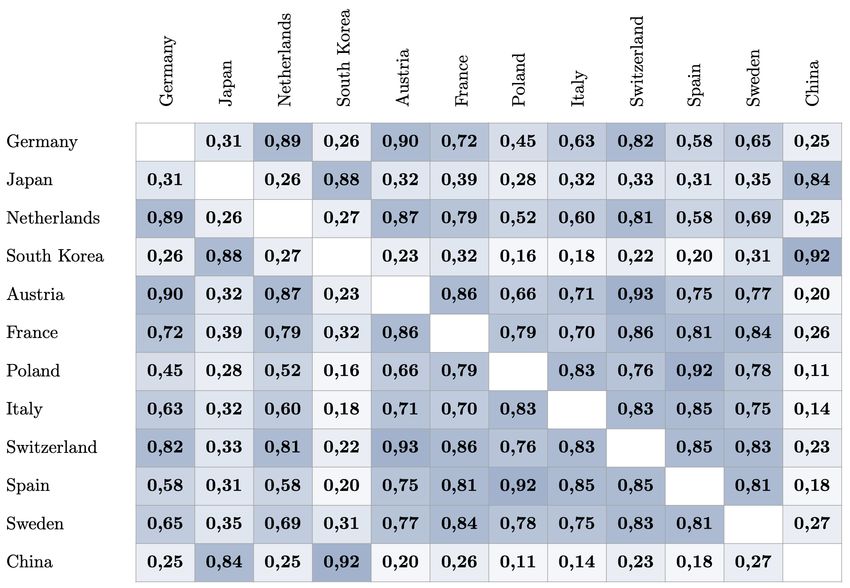
0.12 Figure 6: Similarities in purchase behaviour be-
50000 100000 150000 200000 250000 300000 350000
training size (nbr of examples) tween different markets according to the measure
based on an embedding learned by the neural net-
work.
0.50
0.45
4.2 Cross-market knowledge transfer
catalog coverage
0.40 Categorical cross entropy In this experiment, we first use the similarly mea-
Bayesian personal ranking
sure of Section 3.4 to compare purchase behaviours
0.35 of 12 markets from data of the online store. We
then hypothesise if a model trained with a similar
0.30
market performs better than a model trained to a
dissimilar market.
25000 50000 75000 100000 125000 150000 175000 200000
training size (nbr of examples)
Figure 6 contains computed similarities between
the markets. We note that there is a clear correla-
tion between geographical closeness and similarity
measures. For example, the most similar countries
Figure 5: Validation performance when training to Germany in terms of purchase behaviour are Aus-
with Bayesian personalised ranking loss on Swedish tria and Netherlands, while the most similar mar-
data: top-4 accuracy (left) and catalog coverage kets to China are South Korea and Japan. It is also
(right). possible to see that European markets are similar
to each other while dissimilar to Asian markets.
90.24 tion about how well the recommender system pre-
dicts purchase behaviour in a market.
0.22
To test if our similarity measure is suitable for
top-4 accuracy
0.20
selection, we train three models on data from three
different markets, denoted A, B and C. We then
0.18 evaluate all three models using a validation dataset
from market A. The markets are selected so that
0.16 Sweden
France, 85% similarity A and B have high similarity (> 0.85) according to
Germany, 65% similarity
our measure, and A and C are dissimilar (< 0.65).
50000 100000 150000 200000 250000 300000 350000
training size (nbr of examples) If the similarity measure performs as expected, the
model trained on data from market B should out-
(a) perform the model trained on data from market C
0.22
when validated on market A. We conduct the test
for three different triplets of markets. The results
0.20 are presented in Figure 7.
As baseline, the model is trained and validated on
top-4 accuracy
0.18
data from the same market. This is the same setting
0.16 as in Section 4.1 with results shown in Figure 4a.
We use the baseline to judge how well the models
0.14 Poland
Spain, 92% similarity with data from one market and then validated on
Germany, 45% similarity
0.12 another perform, compared to using data from the
50000 100000 150000 200000 250000 300000
training size (nbr of examples) same market where it is validated.
In figure 7b and 7c the model trained on data
(b) from a similar markets according to the suggested
measure, B, achieves higher Top-K accuracy than
0.26
the model trained on data from a dissimilar market
0.24
C. However, in figure 7a the model trained on data
0.22 from the dissimilar market, C, achieves a slightly
top-4 accuracy
0.20 higher Top-K accuracy than the model trained on
0.18 data from the similar market.
0.16 It is worth noting that there is a significant differ-
Germany
0.14 Netherlands, 89% similarity ence in achieved top-K accuracy between the base-
Spain, 58% similarity
0.12 line and the models trained on data from other mar-
100000 200000 300000 400000 500000 600000
training size (nbr of examples) kets, for all experiments reported in Figure 7. The
exception is the case when data from the Nether-
(c) lands has been used to train a model which has been
validated on data from Germany, where top-K ac-
Figure 7: Top-4 accuracy plotted as a function of curacy levels are very similar.
dataset size when testing how well models trained In all three examples in figure 7 there is a sig-
on data from a secondary market performs on a nificant difference in the top-K accuracy levels be-
local validation dataset. tween the two markets, confirming that from which
secondary market data is used is indeed important.
Our hypothesis is that similarities in purchase be-
haviour could be used do judge if data from one 5 Summary and Conclusion
market could be leveraged for training a recom-
mender system in another market. We conduct an Performance as a function of dataset size In
empirical study for this purpose. We construct a this paper, we show that a recommender system
test to imitate a situation where one small market experience evident saturating effects in validation
(here denoted A) lacks enough data to reach suffi- performance when the size of the training dataset
cient performance levels. To address the shortage, grows. We opted to use a combination of three
data from another similar market is added to the performance metrics, to better estimate quality of
training dataset, to enable training with sufficient the user experience. The three metrics are top-K-
data to reach desirable performance levels on a val- accuracy, catalog coverage and novelty.
idation set. We use top-K accuracy to evaluate this The saturating effect is especially evident in top-
experiment, as it is the metric that gives informa- K-accuracy which approaches a maximum level for
10the specific problem. Furthermore, we observe dif- cal information correlates with purchase behaviour.
ferent behaviours for catalog coverage depending For instance, it predicts that Germany, Nether-
on which dataset we investigate. On the differ- lands, Switzerland and Austria have similar be-
ent datasets from the online store, we observe a haviour. The metric also successfully predicted
decrease in coverage when the amount of training which data would be most successful for knowledge
data increases, while on the yoochoose dataset we transfer in two out of the three tested cases. We
observe a saturating behaviour similar to the top- find these results interesting and promising for fu-
K-accuracy. ture research.
All of our experiments, considering all metrics,
indicate saturating effects on validation data when Conclusion Similar to [19] we conclude that it is
the amount of training data is increased. Our re- not sensible to gather ever increasing amounts of
sults thus further confirm results in [19] and com- data for training recommender systems. When giv-
plement their study in two aspects: evaluating on a ing the user a choice of sharing their personal data
validation set to capture the system’s generalisation for the purpose of personalization, some users will
performance, and evaluating in both accuracy and inevitably opt out. Our results show that this de-
diversity metrics that are purposefully designed to crease in data collected does not necessarily have to
capture good recommendations for the user. be a disadvantage. We have shown that due to sat-
We find that there is an apparent trade-off uration effects in performance there is an amount of
between accuracy-focused metrics such as top-K- data that is enough to reach sufficient performance
accuracy, and diversity-focused metrics such as cat- levels. Secondly, we have shown that if there are
alog coverage and novelty, as indicated in [38]. not enough data available to reach sufficient perfor-
Hence, an optimal amount of data for training can mance levels it is possible to use data from other
be determined if a notion of optimality is clearly similar domains to complete small datasets.
defined: Depending on what is prioritized in the Finally, we propose a metric to judge what do-
system design, the optimal amount of data varies. mains that are similar and where datasets are com-
If accuracy is of high importance more data could patible to a higher extent. The results are promis-
lead to improvements. But if catalog coverage and ing and point us in a direction to further research
novelty are more important, less data could be used on how to efficiently exploit such secondary data
without sacrificing too much accuracy. with transfer learning methods.
From these results, we conclude that sufficient With these results, we believe that there is a
validation performance can be achieved without strong case for working towards minimal necessary
striving towards gathering as much data as possible. data within recommender systems. This has consid-
These results also give room for higher considera- erable privacy benefits without necessarily having
tions of user privacy. Corporations could be more unfavourable effects on performance.
complaint towards users who are hesitant of sharing
their personal data for privacy concerns, without
risking significant performance losses within recom- Acknowledgments
mender systems. We thank Kim Falk for helpful discussions.
Similarity measure and knowledge transfer
We propose a method for constructing a simi- References
larity measure, to measure compatibility between
[1] M. Abadi, A. Chu, I. Goodfellow, H. B. McMa-
datasets in terms of purchase behaviour. First, our
han, I. Mironov, K. Talwar, and L. Zhang.
tests confirm that it is possible to use data from a
Deep learning with differential privacy. In Pro-
secondary market to complement a smaller dataset.
ceedings of the 2016 ACM SIGSAC Conference
Second, we show that validation performance de-
on Computer and Communications Security,
pends on which market the data is taken from, and
pages 308–318, 2016.
that performance varies significantly. In none of our
experiments, the models trained on data from an- [2] M. Al-Rubaie and J. M. Chang. Privacy-
other market were able to perform better than the preserving machine learning: Threats and so-
model trained on data from the original market. lutions. IEEE Security & Privacy, 17(2):49–58,
However, if we trained to a ‘similar’ market, the 2019.
performance was generally better than when train-
ing to a ‘dissimilar’ market. [3] P. Castells, S. Vargas, and J. Wang. Nov-
Our proposed metric shows some promise in the elty and diversity metrics for recommender sys-
sense that it manages to capture how geographi- tems: Choice, discovery and relevance. Pro-
11ceedings of International Workshop on Diver- [14] B. Hidasi, A. Karatzoglou, L. Baltrunas, and
sity in Document Retrieval (DDR), 01 2011. D. Tikk. Session-based recommendations with
recurrent neural networks. arXiv preprint
[4] R. Chow, H. Jin, B. Knijnenburg, and G. Sal- arXiv:1511.06939, 2015.
damli. Differential data analysis for recom-
mender systems. In Proceedings of the 7th [15] B. Hidasi, M. Quadrana, A. Karatzoglou, and
ACM conference on Recommender systems, D. Tikk. Parallel recurrent neural network ar-
pages 323–326, 2013. chitectures for feature-rich session-based rec-
ommendations. In Proceedings of the 10th
[5] P. Cremonesi and R. Turrin. Analysis of cold- ACM conference on recommender systems,
start recommendations in iptv systems. In Pro- pages 241–248, 2016.
ceedings of the third ACM conference on Rec-
ommender systems, pages 233–236, 2009. [16] S. Hochreiter and J. Schmidhuber. Long short-
term memory. Neural computation, 9:1735–80,
[6] K. Falk. Practical Recommender Systems.
12 1997.
Manning Publications, 2019.
[17] W. House. Consumer data privacy in a net-
[7] G. Forman and I. Cohen. Learning from little:
worked world: A framework for protecting pri-
Comparison of classifiers given little training.
vacy and promoting innovation in the global
In European Conference on Principles of Data
digital economy. White House, Washington,
Mining and Knowledge Discovery, pages 161–
DC, pages 1–62, 2012.
172. Springer, 2004.
[8] F. Garcin, B. Faltings, O. Donatsch, A. Alaz- [18] D. P. Kingma and J. Ba. Adam: A method
zawi, C. Bruttin, and A. Huber. Offline and on- for stochastic optimization. arXiv preprint
line evaluation of news recommender systems arXiv:1412.6980, 2014.
at swissinfo.ch. In Proceedings of the 8th ACM [19] M. Larson, A. Zito, B. Loni, and P. Cremonesi.
Conference on Recommender Systems, RecSys Towards minimal necessary data: The case for
’14, page 169–176, New York, NY, USA, 2014. analyzing training data requirements of rec-
Association for Computing Machinery. ommender algorithms. In FATREC Workshop
[9] M. Ge, C. Delgado, and D. Jannach. Beyond on Responsible Recommendation Proceedings,
accuracy: Evaluating recommender systems by 2017.
coverage and serendipity. RecSys’10 - Proceed-
[20] B. Li, Q. Yang, and X. Xue. Can movies and
ings of the 4th ACM Conference on Recom-
books collaborate? cross-domain collaborative
mender Systems, pages 257–260, 01 2010.
filtering for sparsity reduction. In Twenty-First
[10] I. Goodfellow, Y. Bengio, A. Courville, and international joint conference on artificial in-
Y. Bengio. Deep learning, volume 1. MIT press telligence, 2009.
Cambridge, 2016.
[21] A. Maksai, F. Garcin, and B. Faltings. Pre-
[11] K. He, X. Zhang, S. Ren, and J. Sun. Delving dicting online performance of news recom-
deep into rectifiers: Surpassing human-level mender systems through richer evaluation met-
performance on imagenet classification. In Pro- rics. In Proceedings of the 9th ACM Conference
ceedings of the IEEE international conference on Recommender Systems, RecSys ’15, page
on computer vision, pages 1026–1034, 2015. 179–186, New York, NY, USA, 2015. Associ-
ation for Computing Machinery.
[12] J. Hestness, S. Narang, N. Ardalani, G. F. Di-
amos, H. Jun, H. Kianinejad, M. M. A. Pat- [22] B. McMahan, E. Moore, D. Ramage, S. Hamp-
warym, Y. Yang, and Y. Zhou. Deep learn- son, and B. A. y Arcas. Communication-
ing scaling is predictable, empirically. CoRR, efficient learning of deep networks from de-
abs/1712.00409, 2017. centralized data. In Artificial Intelligence and
Statistics, pages 1273–1282. PMLR, 2017.
[13] B. Hidasi and A. Karatzoglou. Recurrent neu-
ral networks with top-k gains for session-based [23] S. M. McNee, J. Riedl, and J. A. Konstan.
recommendations. In Proceedings of the 27th Being accurate is not enough: how accuracy
ACM International Conference on Information metrics have hurt recommender systems. In
and Knowledge Management, pages 843–852, CHI’06 extended abstracts on Human factors
2018. in computing systems, pages 1097–1101, 2006.
12[24] N. Mehrabi, F. Morstatter, N. Saxena, K. Ler- In ICML 2020, 2nd Workshop on Human in
man, and A. Galstyan. A survey on bias and the Loop Learning, 2020.
fairness in machine learning. arXiv preprint
arXiv:1908.09635, 2019. [36] O. Vinyals, Ł. Kaiser, T. Koo, S. Petrov,
I. Sutskever, and G. Hinton. Grammar as a
[25] T. Mikolov, K. Chen, G. Corrado, and J. Dean. foreign language. In Advances in neural infor-
Efficient estimation of word representations in mation processing systems, pages 2773–2781,
vector space. arXiv preprint arXiv:1301.3781, 2015.
2013.
[37] J. Yi, Y. Chen, J. Li, S. Sett, and T. W. Yan.
[26] S. Pan and Q. Yang. A Survey on Trans- Predictive model performance: Offline and on-
fer Learning. IEEE Transactions on Knowl- line evaluations. In Proceedings of the 19th
edge and Data Engineering, 22(10):1345–1359, ACM SIGKDD International Conference on
2010. Knowledge Discovery and Data Mining, KDD
’13, page 1294–1302, New York, NY, USA,
[27] W. Pan. A survey of transfer learning for 2013. Association for Computing Machinery.
collaborative recommendation with auxiliary
data. Neurocomputing, 177:447–453, 2016. [38] T. Zhou, Z. Kuscsik, J.-G. Liu, M. Medo,
J. R. Wakeling, and Y.-C. Zhang. Solv-
[28] W. Pan, N. Liu, E. Xiang, and Q. Yang. Trans- ing the apparent diversity-accuracy dilemma
fer learning to predict missing ratings via het- of recommender systems. Proceedings of the
erogeneous user feedbacks. In IJCAI, 2011. National Academy of Sciences, 107(10):4511–
[29] W. Pan, E. Xiang, N. Liu, and Q. Yang. 4515, 2010.
Transfer learning in collaborative filtering for
sparsity reduction. In Proceedings of the
AAAI Conference on Artificial Intelligence,
volume 24, 2010.
[30] M. Quadrana, A. Karatzoglou, B. Hidasi, and
P. Cremonesi. Personalizing session-based rec-
ommendations with hierarchical recurrent neu-
ral networks. In Proceedings of the Eleventh
ACM Conference on Recommender Systems,
pages 130–137, 2017.
[31] Recsys. Recys 2015 challenge.
https://recsys.yoochoose.net/challenge.html.
Visited on 2020-09-09.
[32] S. Rendle, C. Freudenthaler, Z. Gantner, and
L. Schmidt-Thieme. Bpr: Bayesian person-
alized ranking from implicit feedback. arXiv
preprint arXiv:1205.2618, 2012.
[33] D. Silver, A. Huang, C. J. Maddison, A. Guez,
L. Sifre, G. Van Den Driessche, J. Schrit-
twieser, I. Antonoglou, V. Panneershelvam,
M. Lanctot, et al. Mastering the game of go
with deep neural networks and tree search. na-
ture, 529(7587):484–489, 2016.
[34] Y. K. Tan, X. Xu, and Y. Liu. Improved recur-
rent neural networks for session-based recom-
mendations. In Proceedings of the 1st Work-
shop on Deep Learning for Recommender Sys-
tems, pages 17–22, 2016.
[35] M. Tegnér. Online learning for distributed and
personal recommendations—a fair approach.
13You can also read