Deep-3D Microscope: 3D volumetric microscopy of thick scattering samples using a wide-field microscope and machine learning - arXiv

Deep-3D Microscope: 3D volumetric microscopy
 of thick scattering samples using a wide-field
 microscope and machine learning
 B OWEN L I , 1 S HIYU TAN , 2 J IUYANG D ONG , 3 X IAOCONG L IAN , 1
 YONGBING Z HANG , 4 X IANGYANG J I , 1,* A SHOK V EERARAGHAVAN 2,*
 1 Department of Automation, Tsinghua University, Beijing, China
arXiv:2110.07218v1 [physics.optics] 14 Oct 2021

 2 Department of Electrical and Computer Engineering, Rice University, Houston, TX 77005, USA
 3 Tsinghua Shenzhen International Graduate School, Shenzhen, China
 4 Harbin Institute of Technology (Shenzhen), Shenzhen, China
 * vashok@rice.edu, xyji@tsinghua.edu.cn

 Abstract: Confocal microscopy is the standard approach for obtaining volumetric images of a
 sample with high axial and lateral resolution, especially when dealing with scattering samples.
 Unfortunately, a confocal microscope is quite expensive compared to traditional microscopes. In
 addition, the point scanning in a confocal leads to slow imaging speed and photobleaching due
 to the high dose of laser energy. In this paper, we demonstrate how the advances in machine
 learning can be exploited to "teach" a traditional wide-field microscope, one that’s available in
 every lab, into producing 3D volumetric images like a confocal. The key idea is to obtain multiple
 images with different focus settings using a wide-field microscope and use a 3D Generative
 Adversarial Network (GAN) based neural network to learn the mapping between the blurry
 low-contrast image stack obtained using wide-field and the sharp, high-contrast images obtained
 using a confocal. After training the network with widefield-confocal image pairs, the network
 can reliably and accurately reconstruct 3D volumetric images that rival confocal in terms of
 its lateral resolution, z-sectioning and image contrast. Our experimental results demonstrate
 generalization ability to handle unseen data, stability in the reconstruction results, high spatial
 resolution even when imaging thick (∼ 40 microns) highly-scattering samples. We believe that
 such learning-based-microscopes have the potential to bring confocal quality imaging to every
 lab that has a wide-field microscope.

 © 2021 Optical Society of America under the terms of the OSA Open Access Publishing Agreement

 1. Introduction
 High-throughput, high-resolution, high-contrast microscopy techniques, that do not damage
 tissue are critical for multiple domains including scientific imaging, pathology, medical imaging,
 and in-vivo imaging. The current workhorse of microscopy is a wide-field microscope and
 every science lab, pathologist’s office and hospital/clinic in every corner of the globe likely has
 access to one. While wide-field microscopes have truly been democratized, they are for the most
 part only suited to image the surface of thin samples. 3D volumetric imaging, especially with
 scattering tissue samples is a rapidly growing need that wide-field microscopes cannot address.
 Existing techniques for 3D volumetric imaging in scattering samples such as confocal mi-
 croscopy [1, 2], two-photon microscopy [3–8], and light-sheet microscopy [9–14] all rely on
 more complex optics and illumination designs that end up being prohibitively expensive for
 many parts of the world. The question we ask in this paper is "Can the revolutionary advances in
 machine learning over the last decade be exploited to turn the data acquired from conventional
 wide-field microscopes to rival 3D volumetric data acquired using confocal microscopes — even
 when imaging thick scattering samples?"

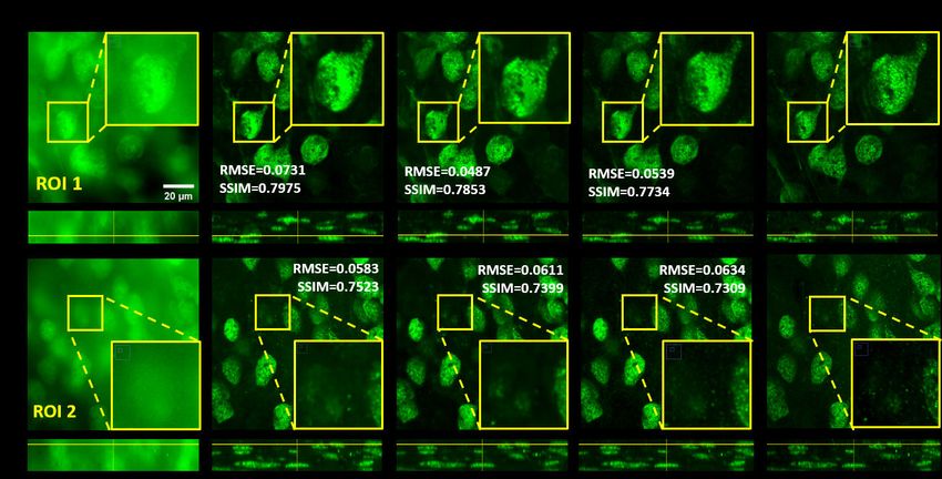
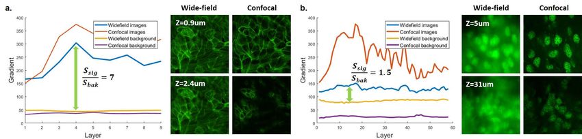
Fig. 1. Sharpness analysis for thin/thick samples. The sharpness of the signal region
 and background noise at different axial depths are plotted. a)The sharpness curves
 for the wide-field and confocal images of a 3-microns MCF10A thin sample. b)The
 sharpness curves for the wide-field and confocal images of a 38-microns neuron thick
 sample. In the thin sample, the molecular structure is clear in the focus plane and less
 influenced by background noise, while the structures in the thick sample is severely
 deteriorated by background and scattering noise.

AI-enhanced fluorescence microscopy. Machine learning and artificial intelligence have made
revolutionary advances in the last decade and have completely transformed a variety of applications
all the way from autonomous vehicles to medical diagnostics. These revolutionary advances have
been the result of (a) new deep neural network architectures that are highly over-parameterized, (b)
datasets acquired to "teach" these networks, and (c) efficient algorithms both for training and for
testing. This AI revolution has also begun to have significant impacts on microscopy, biological
and scientific imaging. The key advantage is that, with no or little modification to conventional
microscopes, AI techniques can provide additional capabilities such as high resolution [15–17],
high SNR [18, 19], fast acquisition [20–22], autofocusing [23, 24], and cross-modality [25–28].
 Over the last few years researchers have developed early examples of deep convolutional
neural networks to enhance axial resolution and imaging contrast of wide-field images [29–33].
Specifically, Zhang et al. [29] first successfully transformed wide-field images to background
reduced Structured Illumination Microscopy (SIM) images using a 2D neural network. However,
their only demonstration was limited to samples with relatively simple structures. Although
they subsequently demonstrated more complicated mice whole-brain images reconstruction
in [31], the 2D convolutional structure confined the application of the network to physically
sectioned tissue samples. Wu et al. proposed two more sophisticated Generative Adversarial
Network (GAN) based deep networks to predict confocal images from a single in-focus wide-field
input [28] and sparse wide-field scans [33], respectively. However, they only testified this idea
using 2.4 microns thickness BPAEC sample or a limited z-span of C-Elegans sample (about 4
microns).
 Here, in our paper, we take a significant leap compared to these related works. While all of
the above approaches were limited in the sample thickness/simple structures, we aim to perform
true three dimensional reconstructions in thick scattering samples (demonstrating 10x thicker
samples than prior work) with more complex structures. In the thick scattering sample, the
images captured by a wide-field microscope are more severely deteriorated by the scattering
background and noise than a thin sample. As show in Figure 1, the contrast (sharpness ratio
between signal region and background region) of wide-field images captured at different axial
layers in a 38-microns neuron slice can be as much as 5× lower than the contrast in a 3-microns
MCF10A thin sample. Molecular structures are submerged in the noisy background of thick
sample, which brings us more difficulties on wide-field to confocal predictions using deep neural
networks. The key technical insight that allows us to move from thin scattering samples to thick
samples, is the idea that in thick samples there is a lot of information cross-talk between and

across sections (z-stack) and 2D neural networks are sub-optimal for capturing the structure
of these complex interactions. We develop a 3D convolutional neural network structure that
allows us to learn statistical relationships across the entire thick sample, allowing high-resolution,
high-contrast 3D reconstructions over the entire volume.
 In particular, we propose a GAN-based three-dimensional (3D) convolutional neural network
(WFCON-Net) that can digitally predict confocal z-stack images from measurements of a wide-
field microscope. We believe this technology will allow widely accessible wide-field microscopes
to capture 3D volumetric imaging datasets of thick scattering samples – with a quality comparable
to (but slightly worse than) a confocal microscope. Our work is inspired and motivated by the
recent work [28] but with three significant contributions. First, we propose a 3D convolutional
network to leverage the inter-layer connections other than recurrent blocks, to utilize the stronger
crosstalks between different layers in thick/dense tissue samples. This strengthens the learning
power to successfully recover fine structures under high magnification with stronger scattering
backgrounds. Second, we add a photo-realistic VGG loss to preserve image high-frequency
details. Third, we propose a 3D tailored registration technique – point spread function (PSF)
based registration to accurately align cross-modality wide-field and confocal image pairs under
high noise disturbance. Furthermore, WFCON-Net can estimate dense confocal z-stacks from
fewer wide-field z-scans, and thereby has the potential for further reducing the sample acquisition
time. Also, we show that WFCON-Net has a good generalization ability to unseen sample
data. Therefore, with the proposed method we can digitally obtain high-resolution confocal
z-stacks using a typical wide-field microscope, without sacrificing the imaging depth, speed,
resolution, or field of view (FOV). In summary, by using the GAN-based 3D convolutional neural
network, together with the VGG loss and the 3D tailored registration techniques, we succeeded in
recovering true 3D confocal fluorescence of thick scattering samples from enormously degraded
wide-field input.

2. Methods
Consider a wide-field microscope imaging a thick scattering tissue sample. Typically the images
obtained will suffer from low-contrast and blur associated with both in-plane and out-of-plane
scattering making images (especially beyond the first 10 microns of tissue) practically un-usable.
Even so, there are significant degrees of freedom in a wide-field microscope that one can take
advantage of. The focus setting of the microscope can be slowly changed from the top to the
bottom of the tissue sample to obtain a low-contrast image stack. Regardless, each image contains
a different but known linear combination of light from the entire 3D tissue sample. The question
we ask, is whether this is sufficient information to de-multiplex and recover a sharp, high-contrast
volumetric image of the sample. In particular, we wish to leverage deep learning techniques and
use a deep generative adversarial network to learn a mapping between the blurry, low-contrast
z-stack obtained using a wide-field microscope and a sharp, high contrast 3D volume imaged
using a confocal microscope.

WFCON-Net architecture. WFCON-Net is a 3D GAN-based deep neural network, whose
architecture is shown in Figure 2. The input to the network is a stack of wide-field images
obtained using a wide-field microscope. The output of the network is the prediction of what the
corresponding sharp, high-contrast 3D volumetric image obtained using a confocal microscope
would be. The network consists of two parts: a generator and a discriminator. The generator takes
3D stacked wide-field fluorescence images as input and outputs corresponding confocal z-stack
images in a single inference. During training, the discriminator similar to [28] is learned to
distinguish confocal ground truths from the predictions. The use of the discriminator encourages
the generator to predict confocal z-stacks with high accuracy, together with appropriate loss
function, providing a good match to ground truth images.

a. Wide-field to confocal transformation (WFCON-Net)
 Wide-field input Generator output Confocal ground truths
 WFCON-Net
 L1 Loss
 (Generator)
 VGG Loss

 GAN Loss

 b. Discriminato
 r Data flow

 Loss calculation

 c.

 3D Conv+LRelu 3D Conv+IN+LRelu+Conv+IN+LRelu
 3D data cube 4D tensor 3D Residual mapping
 AveragePooling 3D FC+LRelu 3D FC+Sigmoid
 3D Maxpooling 3D NN interpolation+Conv
 3D Conv+Relu+Conv+Relu+IN 3D Conv+Relu

 Fig. 2. Overview. a). The WFCON-Net is a 3D GAN-based deep neural network,
 consisting of a generator and a discriminator. The generator takes 3D stacked wide-field
 fluorescence images as input, and outputs corresponding confocal z-stack images in a
 single inference. During training, the discriminator is learned to distinguish confocal
 ground truths from the predictions. The use of the discriminator encourages the
 generator to predict confocal z-stacks with high accuracy, providing a good match to
 ground truth images. b) and c). Network architectures of generator and discriminator.

 The generator is a modified 3D convolutional U-net [34], consisting of an encoder path
followed by a decoder path. The encoder path contains four down-sampling blocks: a max-
pooling layer, two 3x3 3D convolutional layers, an instance normalization layer [35] and a Relu
activation layer [36]. The use of the normalization layer makes the training of thick samples
with diversely distributed signals and strong scattering backgrounds stable. In the decoder
path, the max-pooling layer is symmetrically replaced by a nearest neighbor interpolation layer
followed by a convolution layer with stride 1. The nearest neighbor interpolation layer, in our
case, encourages the upsampling with fewer checkerboard artifacts than transpose convolutions.
Moreover, residual mappings are performed between each convolutional layer to guarantee the
gradient flow. All the convolution and normalization operations are implemented in a 3D manner
to explore the inter-layer relation of the volumetric z-stack data. During training, the loss of the
generator and the discriminator are defined as:
 
 = [ ( ( )) − 1] 2 + 1 ( ( ), ) + ( ( ), )
 (1)
 
 = [ ( ( ))] 2 + [ ( ) − 1] 2

where refers to the wide-field z-stack images, refers to the corresponding sharp images
captured by a confocal microscope, considered as the ground truth. and denote the generator
and the discriminator. The generator loss contains a least-square GAN loss [37] (with an
additional L1 regularizer) and a perceptual VGG loss [38], where and are the corresponding
weights. The use of the perceptual loss encourages high-quality, high-resolution predicted

confocal images. In this paper, we set = 2, = 0.01 for all the experiments.

Training and testing data acquisition. To train/test our network, we captured 39 pairs of
wide-field and confocal z-stacks images (with the lateral size of 2048 × 2048), using a developed
setting of Andor Dragonfly spinning-disk confocal microscope that contains both wide-field
fluorescence image capture mode and confocal fluorescence image capture mode. These image
pairs of different regions of interest (ROIs) were randomly selected with different structures
and neuron densities, covering the characteristics of different part of the tissue slice, and are
split into ’training’ (31 pairs) and ’testing’ (8 pairs) sets. As a similar remark to [34], more data
cannot significantly enhance reconstruction quality but at the price of computational burden.
The z-stacks are scanned with a step size of 0.5 . The number of scans varies from 35 to
76, depending on the distribution of fluorescent signals along the z-axis. The same objective
(60x/1.4NA oil, Nikon) was used for both wide-field and confocal imaging, and the resulting
pixel size (in the image plane) is 108.3 .
 During training, the z-stacks were randomly cropped into 256x256x12 3D data patches. The
data patches were then augmented with random flips and rotations, and normalized to [0, 1]
before inputting to the network. We trained our network for 6000 iterations (equivalent ∼ 60
epochs) using NVIDIA TitanXp GPU and it takes 3 days for training.

Accurate image registration. To ensure the reconstruction quality of thick samples under high
magnification, accurate image registration is indispensable. However, severe background and
decreased contrast in wide-field images make commonly used cross-correlation registration (or
calculate SSIM value) prone to error. Therefore, we proposed a new registration method tailored
for 3D that calculates the PSF between confocal and wide-field image stacks, which can learn
the physical connections between two stacks that is more robust to noise. Then we use this PSF
to determine the lateral and axial shifts. We termed three-dimensional confocal images as ,
wide-field images as . For simplicity, we treat the confocal images as ground-truth of sample
distribution, then = ∗ + , where is the PSF of wide-field images and noise results from
non-uniform system/model errors and randomness of measurement. To robustly recover PSF, we
add standard TV constraints on the gradients of the recovered PSF. Therefore, we can formulate
the objective function as:

 = arg min k − k 22 + k∇ k 1 + k1 − 1k 22 (2)
 
where the first term is the least-squares data fitting term, the second term is TV gradients
penalty, the last term enforces the energy conservation constraint, i.e., Σ , ( , ) = 1. In
this experiment, is set to 1 and is set to 10. We use optimal first-order primal-dual
framework [39, 40] to optimize this objective function to get optimal :
 +1 = ∗ ( + ¯ )
 +1 = ( + ∗ +1 ) (3)
 ¯ = +1 + ( +1 − )
Where , and are hyper-parameters, is gradient operator, ∗ denotes the convex conjugate,
 ∗ and are proximal operators for function ∗ and , exact formula of these two
operators can be found in [39]. Once has been determined, the relative shift between wide-field
and confocal image can be accurately calculated by the shift of maximal intensity point of PSF .
Accurate image registration can substantially enhance the reconstruction quality.

Sample preparation of Immuno-fluorescent staining mouse brain slices. We demonstrated
the performance of WFCON-Net on 40 -thick C57/B6 mouse brain slices obtained from Prof.

Yichang Jia’s lab, Tsinghua University. The neuron body and microglia of the brain slice are
immune-fluorescent stained and the procedures are described as followed.
 First, the brain slices were freshly obtained from Leica vibrating microtome 7000 (after
perfusion-fixed with 4% paraformaldehyde in 1X PBS), and then incubated with permeate-
blocking buffer (0.3% Triton-X100, 3%BSA in 1X PBS) at room temperature for 2 hours. After
that, the slices were gently washed 5 times (5 min per wash) with washing buffer (0.05%Tween-20,
3%BSA in 1X PBS), incubated with NeuN antibody (Cell Signaling #94403, 100X dilution in
washing buffer) and Iba1 antibody (Cell Signaling #17198, 100X dilution in washing buffer) at
4℃for 24 hours, protected from light. On the next day, the slices were gently washed 5 times again
with washing buffer, then incubated with Alexafluor-488 labeled goat-anti-mouse antibody (Cell
Signaling #4408, 200X dilution in washing buffer) and Alexafluor-555 labeled goat-anti-rabbit
antibody (Cell Signaling #4413, 200X dilution in washing buffer) at 4℃overnight in the dark.
On the third day, the slices were gently washed 5 more times with washing buffer, transferred
on Superfrost™ Plus slides, mounted with 22 mm No.1.5 square coverslips, and ProLong Gold
antifade mountant containing 2 µg/mL DAPI. These prepared slices were protected from light
and stored at 4℃before imaging. All the reagents, coverslips, and tissue slides were purchased
from ThermoFisher if mentioned otherwise.

3. Results
3D confocal imaging of mouse brain slices using WFCON-Net. We first demonstrate our
method on a mouse brain slice, as shown in Figure 3a. The model is trained on 31 pairs of the
registered wide-field and confocal z-stack images and tested on the other 8 pairs. The prediction
results, as well as the wide-field inputs, the corresponding confocal ground truths, and the
difference images of the selected region of interest (ROI) with different neuron densities/structures
are shown in Figure 3b. We make use of the root mean square error (RMSE, the lower the
better) and the structural similarity index measure (SSIM, the higher the better) to quantitatively
evaluate the prediction accuracy. The average RMSE and SSIM of the testing datasets are
0.0575 and 0.7673. As we can see from the figure, the mice brain sample we applied is a
thick scattering sample (∼ 40 micron), that the details of the wide-field images are completely
overwhelmed by the scattering background. The predictions of such highly-scattering samples
are significantly challenging than thinner samples (∼ several microns) [28, 31]. Our proposed
GAN-based WFCON-Net, with 3D convolutional operations, can successfully reconstruct the
high-contrast, high-resolution z-stack images from the wide-field captures, matching the confocal
images well at the corresponding planes. The magnified y-z, x-z cross-sections of the image
stacks (span 12 in the z-direction, the full-stack results (over 38 ) are shown in video 1
and 2 in the supplementary), in Figure 3c and d, demonstrate the reconstruction accuracy across
z-axis. The performance for the areas with denser neuron accumulation (such as ROI2) degrades
slightly because of the more rigorous scattering background, leading to a larger reconstruction
RMSE and a lower SSIM.
 Our network also shows good generalization ability to unseen data. Without retraining, we
tested model with images captured from another two neuron slices, which have obviously different
levels of background and scattering. Images of one slice have less background (fig. 4a,b)) while
another suffer from more severe background (fig. 4c,d)). The images are shown in grayscale
to clarify the level of background noise. The reconstructed images show good background
suppression capability with acceptable artifacts. Images of green channel(fig. 4a,c), GFP) exhibit
higher accuracy than blue channel(fig. 4b,d), DAPI) as the same channel used for the training. As
images with more severe background share more similarities with the training set, their inference
results are better than those images with less background. The average RMSE and SSIM of the
testing datasets are 0.0695/0.7153 and 0.0544/0.7501 for green channel and 0.1106/0.6712 and

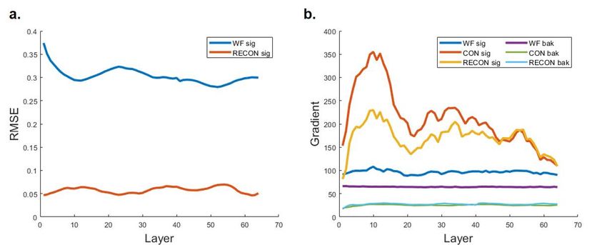
0.0923/0.6527 for blue channel.
 The image quality of inputs together with outputs are affected by the thickness of sample. As
axial depth increases, the sharpness of confocal ground-truth images and the reconstructions are
both deteriorated. However, as shown in Figure 5a, the learning to the confocal ground-truth
remains stable with different depth, which confirms the learning robustness of the proposed
network. Furthermore, we measure the sharpness by calculating the gradient of image patches of
size 32x32 by Δ = |Δ | + |Δ |. In each depth, we take the patch with largest gradient as a
sharpness measurement of signal, and the smallest one as a measurement of background noise.
As shown in Figure 5b, the sharpness of the background keep almost constant while the sharpness
of confocal images is degraded along with depth. Although in superficial layers the confocal
images outperform the network outputs, but they continuously lost superiority when image deeper
because the network can take advantage of a priori knowledge learned from shallower layer,
which is a great advantage of our Deep learning enabled confocal microscope.

WFCON-Net outperforms 2D convolutional networks for thick-sample prediction. Next,
we compare our method with other 2D convolutional GAN-based networks. The prediction
results for DeepZ+ [28], the 2D version of WFCON-Net and our 3D WFCON-Net are shown
in Figure 6. We implemented the DeepZ+ propagation algorithm as proposed in [28], which
takes the single-layer wide-field image as input. The algorithm propagates the single wide-field
image to predict multi-layer confocal z-stacks. Such propagation works well on the thin/sparse
BPAEC microtubule structures, but fails to generate accurate propagation for thick/dense mice
brain samples as shown in Figure 6b. We also investigated the 2D WFCON-Net by replacing
the 3D convolutional blocks with 2D convolutions. Figure 6c and d display the predicted
confocal images of 2D WFCON-Net and 3D WFCON-Net. The yellow boxes show a magnified
view of the cell body and the insets mark the intensity profile of specific regions. Our 3D
convolutional WFCON-Net benefits from the stronger representation ability and inter-layer
correlation information, outperforming the 2D methods in confocal predictions with less blur,
richer details and higher accuracy.

Training with GAN and VGG loss. Moreover, we introduce the perceptual VGG loss together
with GAN loss to train our network. VGG loss is prevalent in natural image super-resolution as it
can enhance the high frequency details that are filtered in low-resolution images, making the
image more realistic [41]. On the contrary, conventional PSNR oriented loss tends to smooth the
reconstruction result [38]. As shown in Figure 7, by adding the VGG loss, the reconstruction
details are well preserved (especially in the overexposed area) and the background noises are well
suppressed. The use of the perceptual loss encourages high-quality, high-resolution predictions,
matching the corresponding confocal images well. The result also demonstrates that different
image generation tasks share some feature similarities.

PSF-based registrations. Image registration is one of the main issues for learning-based
cross-modality image reconstruction. The greater the degree of scattering and noise, the higher
the difficulty for registration. As shown in (fig8.a)), fluorescent structures in the thick sample are
more ambiguous than the thin sample, resulting in the decrease of the accuracy of registration
and the degradation of the reconstruction performance. We can observe that the cross-correlation
curve along the z-axis is flatter than the PSF curve (fig8.b), especially in thick samples. This
flatness causes difficulty identifying the actual shift between image pairs. By calculating the PSF
between 3D wide-field and confocal image pairs, we find the physical connection between two
modalities and the registration process becomes more accurate, and reconstructed details are thus
well preserved (fig8.c). The registration error of the PSF estimation method occurs only when
the shift between wide-field and confocal images falls in the middle of two integer numbers,

corresponding to two peaks with approximate height as shown in the left plot of (fig8.b). Hence,
the maximum theoretical error is nearly half of the minimum z-step size. The PSF registration
error can be further reduced with a smaller z-step size.

Ablation study on the number of wide-field input layers. Our method requires capturing
the whole stack of wide-field images by scanning along the z-direction. To accommodate
the applications that demand faster data acquisition, we investigated the performance of our
network trained with whole dataset but tested with fewer images as input. Specifically, we
subsample the layers of captured z-stacks at an interval of 2 layers (downsample 2x) and 4
layers (downsample 4x), and interpolated the missing layers to the original size before feeding
them into the network. The downsampled z-stacks come with an equivalent z-step of 1 and
2 , respectively (original z-step ∼ 0.5 ). Figure 9 shows the reconstruction results with 2x
downsampling, 4x downsampling, and without downsampling (without retraining the network).
We can see that the model trained for the original data (without downsampling) works well for
the 2x downsampling, and is slightly degraded for 4x downsampled z-stacks. The spacing of 4x
downsampled images in z-axis is comparable to the spacing Huang et al. demonstrated [33],
but we show good results on samples with much more complicated structures and unwanted
backgrounds. The degradation is mainly caused by the gap between captured input layers and the
interpolated layers. Higher reconstruction quality can be obtained if we retrain the network with
the interpolation process included in the pipeline. The average RMSE and SSIM of the testing
dataset for without/2x/4x downsampling are 0.0575/0.0598/0.0657 and 0.7673/0.7343/0.6652,
respectively.

4. Discussion
We provide a GAN-based 3D improved U-Net neural network to generate the confocal images from
the wide-field images. To the best of our knowledge, we are the first to deal with wide-field images
of a thick and complex sample, in which input image quality is severely degraded by scattering
and background noise. By using GAN-based 3D U-Net with additional residual mapping,
normalization layer and VGG loss, together with accurate image registration, the reconstructed
details are repaired from wide-field images. Our model has shown good generalization ability,
either channel generalization or sample generalization, and can also be used with z-downsampled
inputs. Our experimental results demonstrate generalization ability to handle unseen data, stability
in the reconstruction results, high spatial resolution even when imaging thick ( 40 microns)
highly-scattering samples. We believe that such learning-based-microscopes have the potential
to democratize scientific imaging bringing confocal quality imaging to every lab that has a
wide-field microscope.
 Our method is currently limited by the requirement of the training dataset to achieve the best
performance. In some scenarios, like in-vivo neuron activity imaging of moving mice, the ground
truth confocal or two-photon images are hard to acquire and register to the wide-field inputs. If
we using the model trained on another sample, the inference result will be degraded. To deal
with this problem, we can generate images from simulations as in [42] or explore variants of
transfer learning/domain adaptation.

Acknowledgement
We would like to thank Yichang Jia and Xu Zhang from Tsinghua University for their help
on preparing the samples. We would also like to thank Xu Chen from Tsinghua Shenzhen
International Graduate School for preparing the visualization video. In addition, we thank Yanli
Zhang and Yalan Chen from Technology Center for Protein Sciences of Tsinghua University for
assistance of using microscopes.

a. Full FOV fluorescence image b. Wide-field input WFCON-Net output Confocal GT |input-GT| |output-GT|
 1
 ROI 1

 ROI RMSE=0.3140 RMSE=0.0425
 SSIM=0.2890 SSIM=0.7770
 3 0
 1
 ROI 2

 RMSE=0.1925 RMSE=0.0828
 SSIM=0.5154 SSIM=0.6995
 ROI ROI
 0
 1
 4 2 ROI 3
 ROI
 1
 RMSE=0.3250 RMSE=0.0514
 SSIM=0.4201 SSIM=0.7683 0
 1
 ROI 4

 RMSE=0.3763 RMSE=0.0496
 SSIM=0.2842 SSIM=0.7443 0

c. ROI 1 (y-z, z: 2um-14um) ROI 2 (y-z, z: 5um-17um) ROI 3 (y-z, z: 12um~24um) ROI 4 (y-z, z: 20um~32um)
GT Output Input

 Output GT Output GT
d. Input Input Output GT Input Input Output GT
 ROI 3 (x-z, z: 12um~24um)
 ROI 2 (x-z, z: 5um-17um)
 ROI 1 (x-z, z: 2um-14um)

 ROI 4 (y-z, z: 20um~32um)

 Fig. 3. 3D confocal imaging of mouse brain slices using WFCON-Net. a). The
 full field of view (FOV) axial fluorescence image of a mouse brain slice. The full
 image is stitched together from 15 sub-images (for different parts of the slice) captured
 using a 4x/0.2 objective lens. b). Digital confocal predictions using WFCON-Net
 for 4 different ROIs with different neuron densities/structures. The wide-field inputs
 and confocal ground truths are also shown for comparison. The predicted confocal
 images match the ground truths (scanned using a confocal microscope) very well at
 corresponding x-y planes. The root mean square error (RMSE, the lower the better)
 and the structural similarity index measure (SSIM, the higher the better) are used
 here to quantitatively evaluate the prediction accuracy. The cross-sectional images
 span 12 in the z-direction (with a step size of 0.5 ).The error maps |output-GT|
 show that the reconstruction qualities are slightly degraded with the increased neuron
 aggregation. c) Magnified view of y-z cross sections in 4 ROIs same to b show accurate
 three-dimensional confocal image reconstruction. The z-axis spans of those images are
 explicitly labeled. d) Magnified view of x-z cross sections in 4 ROIs same to b.

Fig. 4. Ablation study on model generalization ability. a,b)The green channel(GFP)
and blue channel(DAPI) of wide-field fluorescence images are captured from another
neuron slice with less background. The results show good background noise suppression
capability with acceptable artifacts. c,d) The same setting but using another slice
with more scattering and background than training data. As these images are more
similar to the training data, their inference results are better than those images with less
background.

Fig. 5. Quantitative analysis of network reconstruction along with depth a)The
 average RMSE of wide-field images and recovered images refering to confocal ground-
 truth images along with depth. b)The average sharpness curve of neuron slice wide-field
 images, confocal images, reconstruction images and the corresponding backgrounds.

Disclosures
The authors declare no conflicts of interest.

References
1. T. Wilson, “Confocal microscopy,” San Diego (1990).
2. J. Pawley, Handbook of biological confocal microscopy, vol. 236 (Springer Science & Business Media, 2006).
3. F. Helmchen and W. Denk, “Deep tissue two-photon microscopy,” Nat. methods 2, 932–940 (2005).
4. P. T. So, C. Y. Dong, B. R. Masters, and K. M. Berland, “Two-photon excitation fluorescence microscopy,” Annu.
 review biomedical engineering 2, 399–429 (2000).
5. J.-H. Park, W. Sun, and M. Cui, “High-resolution in vivo imaging of mouse brain through the intact skull,” Proc.
 Natl. Acad. Sci. 112, 9236–9241 (2015).
6. R. Lu, W. Sun, Y. Liang, A. Kerlin, J. Bierfeld, J. D. Seelig, D. E. Wilson, B. Scholl, B. Mohar, M. Tanimoto et al.,
 “Video-rate volumetric functional imaging of the brain at synaptic resolution,” Nat. neuroscience 20, 620–628 (2017).
7. I. N. Papadopoulos, J.-S. Jouhanneau, N. Takahashi, D. Kaplan, M. Larkum, J. Poulet, and B. Judkewitz, “Dynamic
 conjugate f-sharp microscopy,” Light. Sci. & Appl. 9, 1–8 (2020).
8. W. Zong, R. Wu, S. Chen, J. Wu, H. Wang, Z. Zhao, G. Chen, R. Tu, D. Wu, Y. Hu et al., “Miniature two-photon
 microscopy for enlarged field-of-view, multi-plane and long-term brain imaging,” Nat. Methods 18, 46–49 (2021).
9. B.-C. Chen, W. R. Legant, K. Wang, L. Shao, D. E. Milkie, M. W. Davidson, C. Janetopoulos, X. S. Wu, J. A.
 Hammer, Z. Liu et al., “Lattice light-sheet microscopy: imaging molecules to embryos at high spatiotemporal
 resolution,” Science 346 (2014).
10. P. J. Keller, A. D. Schmidt, J. Wittbrodt, and E. H. Stelzer, “Reconstruction of zebrafish early embryonic development
 by scanned light sheet microscopy,” science 322, 1065–1069 (2008).
11. R. M. Power and J. Huisken, “A guide to light-sheet fluorescence microscopy for multiscale imaging,” Nat. methods
 14, 360–373 (2017).
12. L. Gao, L. Shao, C. D. Higgins, J. S. Poulton, M. Peifer, M. W. Davidson, X. Wu, B. Goldstein, and E. Betzig,
 “Noninvasive imaging beyond the diffraction limit of 3d dynamics in thickly fluorescent specimens,” Cell 151,
 1370–1385 (2012).
13. K. McDole, L. Guignard, F. Amat, A. Berger, G. Malandain, L. A. Royer, S. C. Turaga, K. Branson, and P. J. Keller,
 “In toto imaging and reconstruction of post-implantation mouse development at the single-cell level,” Cell 175,
 859–876 (2018).
14. Y. Yue, W. Zong, X. Li, J. Li, Y. Zhang, R. Wu, Y. Liu, J. Cui, Q. Wang, Y. Bian et al., “Long-term, in toto live
 imaging of cardiomyocyte behaviour during mouse ventricle chamber formation at single-cell resolution,” Tech. rep.,
 Nature Publishing Group (2020).
15. Y. Rivenson, Z. Göröcs, H. Günaydin, Y. Zhang, H. Wang, and A. Ozcan, “Deep learning microscopy,” Optica 4,
 1437–1443 (2017).
16. H. Wang, Y. Rivenson, Y. Jin, Z. Wei, R. Gao, H. Günaydın, L. A. Bentolila, C. Kural, and A. Ozcan, “Deep learning
 enables cross-modality super-resolution in fluorescence microscopy,” Nat. methods 16, 103–110 (2019).

a. Wide-field input b. DeepZ+ propagation c. 2D WFCON-Net output d. 3D WFCON-Net output e. Confocal ground truth
 Z=20um Z=20um Z=20um Z=20um Z=20um

 RMSE=0.1200 RMSE=0.0612 RMSE=0.0565
 ROI 1 SSIM=0.5097 SSIM=0.6802 SSIM=0.7356

 Z=24.5um Z=24.5um
 Z=25um Z=24.5um Z=24.5um Z=24.5um
 Z=20um RMSE=0.1651 RMSE=0.0561 RMSE=0.0491
 SSIM=0.3901 SSIM=0.7319 SSIM=0.7495

 x-z x-z x-z x-z x-z

 Z=20um Z=20um Z=20um Z=20um Z=20um

 RMSE=0.0932 RMSE=0.0688 RMSE=0.0598
 ROI 2 SSIM=0.5702 SSIM=0.6872 SSIM=0.7173

 Z=24.5um Z=24.5um Z=24.5um Z=24.5um Z=24.5um

 RMSE=0.1378 RMSE=0.0772 RMSE=0.0717
 SSIM=0.4403 SSIM=0.6641 SSIM=0.6933

 x-z x-z x-z x-z x-z

 Fig. 6. Comparison with other wide-field to confocal cross-modality methods. a).
 Wide-field input images of two ROIs. b). Propagated 3D confocal images using
 DeepZ+ [28]. The DeepZ+ takes the single-layer wide-field image (eg. layer = 20 )
 as input, and outputs the propagated 3D confocal z-stacks (only layer = 24.5 
 is shown). The propagation fails to generate accurate predictions for thick samples
 (due to the distributed fluorescence signals in multiple layers and the strong scattering
 background). C). Predicted confocal images using WFCON-Net2D. The WFCON-
 Net2D (with 2D Conv blocks) takes the wide-field z-stacks as input, and predicts the
 corresponding confocal images in a layer-to-layer manner. d). Predicted confocal
 images using WFCON-Net. The WFCON-Net (with 3D Conv blocks) benefits from
 the stronger representation ability and inter-layer correlation information, and thus
 surpasses 2D methods in confocal predictions with higher accuracy and richer details,
 which can be verified by the line profile marked by two triangular arrows in the insets
 of images. e). Confocal ground truth images. For all the images, the x-y images at
 = 20 , 24.5 and their corresponding x-z cross-sections are shown.

Fig. 7. Training with GAN and VGG loss. We use the sum of L1 loss, VGG loss
 and GAN loss as our loss function during training. The use of perceptual loss (VGG
 loss) encourages predictions with higher quality and richer details. a). Wide-field input
 inputs of two different ROIs. b). Predicted confocal images of the network trained with
 only L1 loss [31]. c). Predicted confocal images of the network trained with L1 loss and
 GAN loss [28]. d). Our method, trained with a combination of L1 loss, VGG loss and
 GAN loss. e). Confocal ground truth images. Although the use of non-PSNR oriented
 perceptual loss will slightly affect SSIMs and RMSEs, but as shown in the magnified
 views, our method can reconstruct more details (especially in the overexposed areas –
 ROI1) and suppress more background noises (ROI2).

17. H. Zhang, Y. Zhao, C. Fang, G. Li, M. Zhang, Y.-H. Zhang, and P. Fei, “Exceeding the limits of 3d fluorescence
 microscopy using a dual-stage-processing network,” Optica 7, 1627–1640 (2020).
18. A. Goy, K. Arthur, S. Li, and G. Barbastathis, “Low photon count phase retrieval using deep learning,” Phys. review
 letters 121, 243902 (2018).
19. M. Weigert, U. Schmidt, T. Boothe, A. Müller, A. Dibrov, A. Jain, B. Wilhelm, D. Schmidt, C. Broaddus, S. Culley
 et al., “Content-aware image restoration: pushing the limits of fluorescence microscopy,” Nat. methods 15, 1090–1097
 (2018).
20. W. Ouyang, A. Aristov, M. Lelek, X. Hao, and C. Zimmer, “Deep learning massively accelerates super-resolution
 localization microscopy,” Nat. biotechnology 36, 460–468 (2018).
21. E. Nehme, D. Freedman, R. Gordon, B. Ferdman, L. E. Weiss, O. Alalouf, T. Naor, R. Orange, T. Michaeli, and
 Y. Shechtman, “Deepstorm3d: dense 3d localization microscopy and psf design by deep learning,” Nat. Methods 17,
 734–740 (2020).
22. X. Li, J. Dong, B. Li, Y. Zhang, Y. Zhang, A. Veeraraghavan, and X. Ji, “Fast confocal microscopy imaging based on
 deep learning,” in 2020 IEEE International Conference on Computational Photography (ICCP), (IEEE, 2020), pp.
 1–12.
23. Y. Wu, Y. Rivenson, Y. Zhang, Z. Wei, H. Günaydin, X. Lin, and A. Ozcan, “Extended depth-of-field in holographic
 imaging using deep-learning-based autofocusing and phase recovery,” Optica 5, 704–710 (2018).
24. H. Pinkard, Z. Phillips, A. Babakhani, D. A. Fletcher, and L. Waller, “Deep learning for single-shot autofocus
 microscopy,” Optica 6, 794–797 (2019).
25. C. Ounkomol, S. Seshamani, M. M. Maleckar, F. Collman, and G. R. Johnson, “Label-free prediction of three-
 dimensional fluorescence images from transmitted-light microscopy,” Nat. methods 15, 917–920 (2018).
26. E. M. Christiansen, S. J. Yang, D. M. Ando, A. Javaherian, G. Skibinski, S. Lipnick, E. Mount, A. O’Neil, K. Shah,
 A. K. Lee et al., “In silico labeling: predicting fluorescent labels in unlabeled images,” Cell 173, 792–803 (2018).
27. Y. Rivenson, H. Wang, Z. Wei, K. de Haan, Y. Zhang, Y. Wu, H. Günaydın, J. E. Zuckerman, T. Chong, A. E. Sisk
 et al., “Virtual histological staining of unlabelled tissue-autofluorescence images via deep learning,” Nat. biomedical
 engineering 3, 466 (2019).
28. Y. Wu, Y. Rivenson, H. Wang, Y. Luo, E. Ben-David, L. A. Bentolila, C. Pritz, and A. Ozcan, “Three-dimensional

a 89% 88% c Wide-field input Confocal GT

 Wide-field

 Confocal
 76%

 50%
 Thin sample (MCF10A)
 Wide-field

 Confocal

 Thick sample (brain
 slice) Prediction with Prediction with cross-
 PSF registration correlation registration
 b

 RMSE=0.0550 RMSE=0.0720
 SSIM=0.7340 SSIM=0.7078

 Fig. 8. Image registration with estimated PSF. We register images by estimating the
 3D point spread functions (PSF) from paired wide-field and confocal z-stack images.
 The peak of the calculated PSF profile is then used to determine the lateral and axial
 shifts between unregistered images. a). We compare the PSF registration method with
 the cross-correlation method for thin sample (MCF10A, 3-microns thickness) and thick
 sample (brain slice, 38-microns thickness), respectively. The PSF registration (orange)
 outperforms the cross-correlation method (blue) in higher z-axis accuracy, especially
 for the thick samples. b). Profiles along the z-axis of cross-correlation and calculated
 PSF for the thin sample (left) and the thick sample (right). The sharp peak of PSF
 benefits the accurate registration and is robust to noises across wide-field and confocal
 images. c). WFCON-Net predictions with and without PSF registered training data.
 The PSF registration method improves the reconstruction quality. The ground-truth
 registrations are manually aligned.

 virtual refocusing of fluorescence microscopy images using deep learning,” Nat. methods 16, 1323–1331 (2019).
29. X. Zhang, Y. Chen, K. Ning, C. Zhou, Y. Han, H. Gong, and J. Yuan, “Deep learning optical-sectioning method.”
 Opt. Express (2018).
30. S. Lim, H. Park, S. Lee, S. Chang, B. Sim, and J. C. Ye, “Cyclegan with a blur kernel for deconvolution microscopy:
 Optimal transport geometry,” IEEE Transactions on Comput. Imaging 6, 1127–1138 (2020).
31. K. Ning, X. Zhang, X. Gao, T. Jiang, H. Wang, S. Chen, A. Li, and J. Yuan, “Deep-learning-based whole-brain
 imaging at single-neuron resolution,” Biomed. Opt. Express 11, 3567–3584 (2020).
32. J. Lim, A. B. Ayoub, and D. Psaltis, “Three-dimensional tomography of red blood cells using deep learning,” Adv.
 Photonics 2, 026001 (2020).
33. L. Huang, H. Chen, Y. Luo, Y. Rivenson, and A. Ozcan, “Recurrent neural network-based volumetric fluorescence
 microscopy,” Light. Sci. & Appl. 10, 1–16 (2021).
34. Ö. Çiçek, A. Abdulkadir, S. S. Lienkamp, T. Brox, and O. Ronneberger, “3d u-net: learning dense volumetric
 segmentation from sparse annotation,” in International conference on medical image computing and computer-assisted
 intervention, (Springer, 2016), pp. 424–432.
35. D. Ulyanov, A. Vedaldi, and V. Lempitsky, “Instance normalization: The missing ingredient for fast stylization,”
 arXiv preprint arXiv:1607.08022 (2016).
36. X. Glorot, A. Bordes, and Y. Bengio, “Deep sparse rectifier neural networks,” in Proceedings of the fourteenth
 international conference on artificial intelligence and statistics, (2011), pp. 315–323.
37. X. Mao, Q. Li, H. Xie, R. Y. Lau, Z. Wang, and S. Paul Smolley, “Least squares generative adversarial networks,” in
 Proceedings of the IEEE international conference on computer vision, (2017), pp. 2794–2802.
38. J. Johnson, A. Alahi, and L. Fei-Fei, “Perceptual losses for real-time style transfer and super-resolution,” in European
 conference on computer vision, (Springer, 2016), pp. 694–711.
39. F. Heide, M. Rouf, M. B. Hullin, B. Labitzke, W. Heidrich, and A. Kolb, “High-quality computational imaging
 through simple lenses,” ACM Transactions on Graph. (TOG) 32, 1–14 (2013).

a. Wide-field input b. Confocal GT c. w/o Downsample d. Downsample 2x e. Downsample 4x
Z=7um

Z=16um

Z=22um

 x-z x-z x-z x-z

 Fig. 9. Ablation study on the number of wide-field input layers (along z). We test
 our algorithm with the different levels of input layers by downsampling the wide-field
 z-stacks, without retraining the network. The whole z-stacks are reinterpolated from
 the downsampled data before input to our network. a) Wide-field inputs at different
 depths. Two specific regions of interest (bounded by the blue and yellow boxes) are
 enlarged to show details. The x-z cross-sections are also shown for localization. b)
 Confocal (ground truth, GT) images of the two enlarged regions. c) WFCON-Net
 reconstructed images without downsampling. d) WFCON-Net reconstructed images
 with 2x downsampled input and interpolation. The results are comparable to the results
 without downsampling. e) WFCON-Net reconstructed images with 4x downsampled
 input and interpolation. The reconstruction accuracy degrades slightly and mainly in
 out-of-focus layers, since these layers are more vulnerable to the background signals
 originated from the in-focus layers.

40. A. Chambolle and T. Pock, “A first-order primal-dual algorithm for convex problems with applications to imaging,” J.
 mathematical imaging vision 40, 120–145 (2011).
41. C. Ledig, L. Theis, F. Huszar, J. Caballero, A. Cunningham, A. Acosta, A. Aitken, A. Tejani, J. Totz, and Z. Wang,
 “Photo-realistic single image super-resolution using a generative adversarial network,” IEEE Comput. Soc. (2016).
42. Z. Pengcheng, S. L. Resendez, R. R. Jose, J. C. Jimenez, S. Q. Neufeld, G. Andrea, F. Johannes, E. A. Pnevmatikakis,
 G. D. Stuber, and H. a. Rene, “Efficient and accurate extraction of in vivo calcium signals from microendoscopic
 video data,” Elife 7 (2018).