MVFUSENET: IMPROVING END-TO-END OBJECT DETECTION AND MOTION FORECASTING THROUGH MULTI-VIEW FUSION OF LIDAR DATA - RESEARCHGATE
←
→
Page content transcription
If your browser does not render page correctly, please read the page content below
MVFuseNet: Improving End-to-End Object Detection and
                                                       Motion Forecasting through Multi-View Fusion of LiDAR Data

                                               Ankit Laddha, Shivam Gautam, Stefan Palombo, Shreyash Pandey, Carlos Vallespi-Gonzalez
                                                                                 Aurora Innovation
                                                                   aladdha,sgautam,spalombo,spandey,cvallespi@aurora.tech
arXiv:2104.10772v1 [cs.CV] 21 Apr 2021

                                                                  Abstract

                                             In this work, we propose MVFuseNet, a novel end-to-
                                         end method for joint object detection and motion forecast-
                                         ing from a temporal sequence of LiDAR data. Most existing
                                         methods operate in a single view by projecting data in either
                                         range view (RV) or bird’s eye view (BEV). In contrast, we
                                         propose a method that effectively utilizes both RV and BEV
                                         for spatio-temporal feature learning as part of a temporal
                                         fusion network as well as for multi-scale feature learning in
                                         the backbone network. Further, we propose a novel sequen-
                                         tial fusion approach that effectively utilizes multiple views
                                         in the temporal fusion network. We show the benefits of
                                         our multi-view approach for the tasks of detection and mo-
                                         tion forecasting on two large-scale self-driving data sets,
                                         achieving state-of-the-art results. Furthermore, we show
                                         that MVFusenet scales well to large operating ranges while
                                         maintaining real-time performance.
                                                                                                              Figure 1: The input to our method is a temporal sequence of
                                                                                                              3D native range view images from LiDAR (top) and the out-
                                         1. Introduction                                                      put is object detections and motion predictions in the Carte-
                                            Object detection and motion forecasting are of                    sian bird’s eye view (bottom). In contrast to previous single
                                         paramount importance for autonomous driving. Object de-              view methods, we propose to process the sequence in both
                                         tection entails recognizing and localizing objects in the            views (middle).
                                         scene, whereas motion forecasting entails predicting the fu-
                                         ture trajectory of the detected objects. Traditionally, cas-         spective range view (RV). However, since most planning
                                         caded approaches treat detection and motion forecasting              algorithms operate in the Cartesian bird’s eye view (BEV)
                                         as two separate tasks, which enables classical methods for           space, the object detections and their forecasts need to also
                                         detection and motion forecasting to be used. However,                be in the same Cartesian space (see Figure 1). There-
                                         these methods optimize for these tasks separately, suffer-           fore, every method converts perspective RV information to
                                         ing from cascading errors and missing the opportunity to             a Cartesian BEV at some stage during its processing. Most
                                         share learned features for both tasks [1]. To overcome               existing methods lie on the extreme ends of the spectrum
                                         these issues, multiple end-to-end methods have been pro-             with respect to when they perform this conversion during
                                         posed [2, 3, 4, 5] for jointly solving both detection and mo-        their processing, and most use a single view entirely. On
                                         tion forecasting. These methods have demonstrated excel-             one hand, methods such as [3, 6, 7] process LiDAR data ex-
                                         lent performance [1] while operating in real-time. Follow-           clusively in RV and only convert their final output to BEV
                                         ing the end-to-end paradigm, we propose a novel method               during post processing. These methods are efficient for pro-
                                         for jointly detecting objects and predicting their future tra-       cessing large spatial regions due to the compact size of the
                                         jectories using time-series LiDAR data.                              input image and offer state-of-the-art performance in the
                                            The input LiDAR data is natively captured in the per-             detection of small objects (e.g., pedestrians, bikes) and far

                                                                                                          1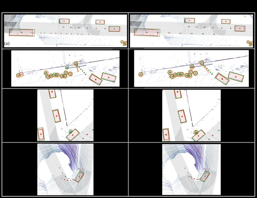
away objects. On the other hand, methods such as [2, 4, 8]               Recently, [10] proposed a multi-view approach for the
project the LiDAR data in the BEV first, with minimal or no           joint task. In this method, the authors proposed fusing a
pre-processing in RV, and perform most of the processing in           single-frame RV projection with multiple frames of BEV
BEV. The Cartesian BEV has the advantage of a strong prior            projection, which improves object detection performance.
due to range invariance of object shape and motion. This              This method, however, limits the temporal fusion of Li-
provides an edge to existing BEV methods on motion fore-              DAR data to BEV and only employs RV features of a sin-
casting tasks; however, their scalability to operate in large         gle sweep, missing high resolution motion cues. In con-
areas remains a challenge. There has been some recent work            trast, our proposed method performs spatio-temporal fusion
on using multiple views for detection [9, 10], but the space          of both BEV and RV features for multiple frames of Li-
of models that can efficiently use multiple views for end-to-         DAR data. To the best of our knowledge, this is the first
end detection and motion forecasting remains largely unex-            method that exploits multiple views for both temporal fu-
plored.                                                               sion and multi-scale backbone feature learning. We show
   Given the complementary benefits of processing in both             that this leads to better detection and motion forecasting
views, we posit that effectively combining both of them can           performance.
lead to improved performance in both detection and fore-
                                                                      2.2. Motion Forecasting
casting. Therefore, in this work we propose MVFuseNet, a
novel end-to-end joint object detection and motion forecast-              Traditional learning-based motion forecasting ap-
ing method which achieves state-of-the-art results on two             proaches [25, 26, 27, 28] use temporal sequences of detec-
large scale data sets and has real-time performance when              tions [7, 8, 21, 29] to learn spatio-temporal features for each
processing a large spatial region. To accomplish this, we             object. Recent work in traditional motion forecasting has
propose a novel sequential multi-view (MV) fusion network             focused on improving the modeling of uncertainty through
to aggregate a temporal sequence of LiDAR data for learn-             multi-modality [30, 31, 32, 28, 33, 34, 35, 36] and interac-
ing spatio-temporal features. We further propose a multi-             tions between actors and the scene [26, 27, 37, 38, 39, 40].
view backbone network to process the spatio-temporal fea-             In contrast, we look at the complementary problem of learn-
tures for detection and forecasting. We demonstrate the ef-           ing better spatio-temporal object features for forecasting
fectiveness of multiple views over a single view on multiple          using sensor data. Our proposed method can also benefit
data sets with different characteristics and LiDAR resolu-            from many of the recent advances in the motion forecasting
tions.                                                                literature. However, to simplify the experimentation, we
                                                                      leave their incorporation to future work. These traditional
2. Related Work                                                       methods are successful in capturing complex relationships
   In this section, we first discuss the existing literature on       and generating realistic longer-term forecasts, but they
LiDAR representation, and then look at various approaches             suffer from cascading error issues [1] and lose out on the
for motion forecasting.                                               rich features learned from sensor data. These methods also
                                                                      work on a per-object basis, which makes them hard to scale
2.1. LiDAR representation                                             to dense, urban environments.
    A spinning LiDAR captures data as a multi-channel im-                 To address the issues with traditional forecasting ap-
age of range measurements. In the literature, these range             proaches, the seminal work by [41] proposed to jointly
measurements have been represented in various ways for                solve both object detection and motion forecasting. [2] im-
processing: unstructured 3D point clouds [11, 12], 3D vox-            proved upon [41] by incorporating scene information using
els [13, 14], a 2D BEV grid [8, 15, 16] and the native 2D RV          a semantic and geometric HDMap. Approaches such as [4]
grid [7, 17, 18, 19]. The point cloud and voxel based meth-           and [1] build on top of [2] by adding an object-centric sub-
ods are computationally expensive and do not scale well to            network to refine future trajectories. These methods show
highly dynamic and crowded outdoor scenes. In compar-                 that recent work on multi-modal predictions and the use of
ison, 2D BEV or RV grid based methods are efficient but               interaction graphs to model complex relationships can be
only use a single view (either BEV or RV) for processing Li-          easily extended to the framework of joint object detection
DAR data. Recent work has investigated the use of multiple            and motion forecasting. [5] and [10] are recent multi-sensor
views [20, 21, 22, 23, 24] and shown that the complemen-              methods that build on top of [4] by using radar and camera
tary benefits of both views improve performance. However,             inputs respectively. These methods, by virtue of operating
these methods use only one frame of LiDAR data and only               in BEV, lose out on high-resolution point information and
solve perception tasks such as object detection and seman-            are often limited by range of operation. RV based methods
tic segmentation. In contrast, we propose a method which              such as [6] and [3] overcome the limitation on operating
aggregates data from multiple frames to jointly solve both            range but are outperformed in the motion forecasting task
detection and motion forecasting in an end-to-end method              by recent BEV based methods. In this work, we improve
by utilizing both the BEV and RV.                                     the joint framework by including multi-view representation

                                                                  2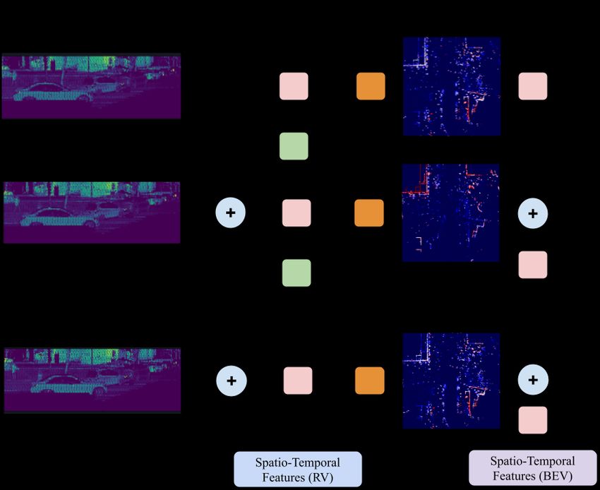
(a) Multi-View Temporal Fusion Network                            (b) Multi-View Backbone Network

Figure 2: MVFuseNet Overview: We propose a novel approach for (a) multi-view temporal fusion of LiDAR data in RV
and BEV to learn spatio-temporal features. We sequentially aggregate sweeps by projecting the data from one sweep to the
next sweep in the temporal sequence. (b) These multi-view spatio-temporal features are further processed by a multi-view
backbone to combine them with map features and learn multi-scale features for final detection and motion forecasting.

in multiple parts of the network and achieve state-of-the-art       points, Sk = {pik }N    k
                                                                                          i=1 , using the pose (viewpoint) of the
performance on both object detection and motion forecast-           sensor Pk at the end of sweep capture. We assume that
ing while scaling to large areas of operation in real-time.         pose for each sweep is provided by an onboard localization
                                                                    system. Therefore, we can calculate the transformation of
3. MV Detection and Motion Forecasting                              points from one viewpoint to another. We denote the k-th
    Figure 2 shows an overview of our proposed approach.            sweep transformed into the n-th sweep’s coordinate frame
Our main contribution is an end-to-end object detection and         as, Sk,n = {pik,n }N                             i
                                                                                        i=1 , where each point pk,n is represented
                                                                                          k

motion forecasting method that processes the time-series            by its 3D coordinates, [xik,n , yk,n
                                                                                                      i     i
                                                                                                         , zk,n  ]T . In spherical co-
LiDAR data in both range view and bird’s eye view. We                                             i
                                                                    ordinates the same point pk,n can be represented using the
first describe prerequisite information related to the input                         i
                                                                    radial distance rk,n             i
                                                                                         , azimuth θk,n   and elevation φik,n . Note
and view-projections in Section 3.1. We then discuss our            that pik,n represents the same LiDAR return as pik , only
contribution of using multiple views for temporal fusion of         transformed into a different frame.
a sequence of LiDAR data in Section 3.2. In Section 3.3, we
                                                                        Projections: For each point pik captured at pose Pk , the
discuss our contribution of a multi-view backbone network
                                                                    range view projection at pose Pn is defined by discretiz-
to extract per-cell features. Finally, we present our method
                                                                    ing the azimuth and elevation angles of pik,n . Similarly, the
for joint detection and motion forecasting using the per-cell
                                                                    bird’s eye projection at pose Pn is the x and y coordinates
features in section 3.4, followed by the loss functions used
                                                                    of pik,n .
to train the model in Section 3.5.
                                                                        Per-Point Features: For each point pik in Sk , we define
3.1. Preliminaries                                                  a set of associated features as concatenation of its coordi-
   Input: Let us assume that we are given a time-series             nates in original viewpoint, [xik,k , yk,k
                                                                                                            i      i
                                                                                                                , zk,k ]T , coordinates
of K + 1 sweeps, where each sweep contains all the Li-              in most recent viewpoint, [xik,0 , yk,0
                                                                                                         i      i
                                                                                                             , zk,0 ]T and the remis-
DAR points from a full 360◦ rotation of a LiDAR sensor.                                i
                                                                    sion or intensity ek of the LiDAR return.
This time series LiDAR data can be denoted by {Sk }0k=−K ,
where k = 0 is the most recent sweep and −K ≤ k ≤ 0                 3.2. Multi-View Temporal Fusion Network
are the past sweeps. We term the most recent sweep as the              The goal of the temporal fusion sub-network is to aggre-
reference sweep. Each LiDAR sweep contains Nk range                 gate a time-series of LiDAR data in order to learn spatio-
measurements, which can be transformed into a set of 3D             temporal features. The most straightforward approach, as

                                                                3
employed by many previous works [2, 4, 6], is the one-
shot approach where all the data is accumulated in a sin-
gle frame. All points are first transformed into the frame
defined by the reference pose and then the aggregation is
done by projecting them in either BEV or RV. For multiple
views this can be trivially extended by projecting the points
in both BEV and RV for aggregation. However, directly
projecting all the past LiDAR data into the RV of the most
recent sweep leads to significant performance degradation
due to heavy data loss in the projection step [3]. There-
fore, instead of previous approaches that focus on one-shot
projection, we propose a novel sequential multi-view fusion
approach to effectively aggregate the temporal LiDAR data. Figure 3: Network Components: (a) We use the depicted
per-sweep network to process each sweep during temporal
Figure 2a shows our proposed fusion approach. We as-
fusion in both views. Note that no weights are shared across
sume that the input is a time-series of multi-channel RV
time and views during temporal fusion. (b) The HDMap is
images in their original capture pose. These images con-
processed with the depicted network to learn local map-only
tain the per point features, fki , as defined in Section 3.1.
features which are combined with the LiDAR features. (c)
We sequentially fuse the LiDAR sweeps from one time-step
The asymmetric U-Net network is used to extract and com-
to the next in both views. At each time-step we warp the
bine multi-scale features in BEV. In RV, only the width di-
previous time-step’s RV features to the current time-step’s
mension is down-sampled and the first convolutional layer
frame (green box), and then use a sub-network (see Fig-
is not strided. Each layer in the networks is represented as
ure 3a) to learn spatio-temporal features for each cell in RV
B, k × k, /s, C, N , where B is the block name, k is the ker-
(pink box). These learned features are then projected into
nel size, s is the stride, C is the number of channels and
the BEV (orange box) and concatenated with the BEV fea-
N is the number of repetitions of the block. Conv denotes
tures from the previous time-step. Similarly to RV, a sub-
a convolutional layer followed by batch normalization and
network is then used to learn spatio-temporal features for
ReLU. Res denotes a residual block as defined in [42]. Fi-
each cell in BEV. The feature learning networks (pink box)
nally, we up-sample using bi-linear interpolation.
in each view and time-step are independent and no weights
are shared across time or view. It is important to note that
RV features of the point gki . For aggregating the features of
unlike previous methods that project raw point-features to
all the points in the cell we use:
the BEV, our method projects learned RV features to be
used in the BEV. We further discuss the methods used to M
i 1 X
warp features from one RV to another and for projecting Bk,0 (lk,0 )= MLP(hik ), (1)
the RV features to BEV. M i=0
RV-to-RV Feature Warping: Let us assume that we
would like to warp the RV feature map Rk,k of kth sweep where MLP is a linear layer followed by batch normal-
to the RV feature map Rk,n at viewpoint on nth sweep. We ization and ReLU.
assume that the point pik is projected to location lk,k i
in Rk,k 3.3. Multi-View Backbone Network
i
and lk,n in Rk,n . Therefore, we define the feature warping The goal of the backbone is to process the spatio-
by copying the features from one RV to another such that temporal features and combine them with map features to
i i
Rk,n (lk,n ) = Rk,k (lk,k ). Similar to [3, 7], if more than learn per-cell features that can be used for object detection
i
one point project into the same cell location lk,n , we pick and motion forecasting. As shown in Figure 2b, our back-
the closest point for feature rendering. bone network processes the spatio-temporal features in both
RV-to-BEV Feature Warping: Let us assume that we views. We first take the spatio-temporal features in RV as
would like to warp the RV feature map Rk,k of kth sweep to input and learn multi-scale RV features by extracting and
the BEV feature map Bk,0 . We also assume that a point pik combining features using an asymmetrical U-Net (see Fig-
in Sk can be projected in Rk,k to extract a learned feature ure 3c). These RV features are then projected to BEV using
gki . We calculate the features of cell lk,0
i
in Bk,0 by aggregat- the same technique as in Section 3.2 and concatenated with
ing the features of all the points Ak = {pik , i = 1, ..., M }
l
learned map features and the spatio-temporal BEV features
that are projected into that cell location. Similarly to [8, 21], (see Figure 2b). We rasterize the map features in BEV [2, 4]
for each point in a cell, we calculate its feature vector hik by and learn high level features using a convolutional neural
concatenating the difference between the coordinates of the network (see Figure 3b). Similar to RV, this multi-view,
point and the cell ∆c = [xik − lx,k,0i
, yki − ly,k,0
i
], and the multi-sensor feature volume is further processed by another
4asymmetrical U-Net to learn multi-scale features in BEV of 200m length. On both data sets, we report results on
(see Figure 3c). three major classes of traffic participants: vehicles, pedes-
trians and bikes.
3.4. Output Prediction Following previous works [1, 4, 3], we use average pre-
Given the per cell features from the backbone network, cision (AP) with intersection over union (IoU) based associ-
our goal is to detect objects observed in the current sweep ation between ground truth and the detected object. Further-
S0 and predict their trajectory. We use a dense, single-stage more, we use L2 displacement error at multiple time hori-
convolutional header for detecting objects using the per-cell zons to evaluate motion forecasting. We compute L2 as the
features. Similarly to [4, 43], we first predict if a cell con- Euclidean distance between the center of the predicted true
tains the center of an object for some class. For each center positive box and the associated ground truth box. Note that
cell, we then predict an associated bounding box and use the official nuScenes leaderboard evaluates the task of de-
non-maximum suppression to remove duplicates. For mo- tection and state estimation, whereas in this work we solve
tion forecasting of large objects such as vehicles, we extract the joint task of detection and motion forecasting. There-
a rotated region of interest (RROI) [1, 4] of 60 × 60m cen- fore, we use the same metrics as used in previous work [1, 2]
tered at the object to learn actor-centric features which are instead of the official leaderboard metrics.
then used to predict the trajectory. However, for smaller ob-
jects such as pedestrians and bicycles, we use the features of 4.2. Implementation Details
the center cell to predict the trajectory since we empirically We use the PyTorch [47] library for implementing the
found that this leads to better results. proposed approach. On nuScenes, the input RV is chosen
to be of size 32 × 1024 based on the LiDAR characteris-
3.5. End-to-End Training
tics. Furthermore, the input BEV feature map is chosen
Similarly to [4, 5]. we train the proposed method end-
to be 400 × 400 and the backbone output is chosen to be
to-end using a multi-task loss incorporating both detection
200 × 200, to balance runtime and resolution. This results
and trajectory loss: Ltotal = Ldet + Ltraj .
in an input resolution of 25cm and an output resolution of
Detection Loss (Ldet ) is a multi-task loss defined as a
50cm. On our internal data set, the input RV is 64 × 2048
weighted sum of classification and regression loss: Ldet =
reg and both the input BEV and output BEV feature map are of
Lcls
det + λLdet . We use focal loss [44] for classifying if a the size 400 × 400. Due to the large ROI, this results in a
BEV cell is at the center of an object class. For each cen-
resolution of 50cm at both input and output. For both data
ter cell, we use smooth L1 loss to learn parameters of the
sets, we use the LiDAR data from the past 0.5 seconds as
object bounding box relative to that cell. We parameter-
input and predict the trajectory for 3 seconds into the future,
ize each box i by it’s center (xi , yi ), orientation (θi ) and
sampled at 10Hz. Since nuScenes is much smaller than our
size (wi , hi ). The orientation is further parameterized as
internal data set, we use data augmentation during training.
(cos(θi ), sin(θi )).
Specifically, we generate labels at non-key frames by lin-
Trajectory Loss (Ltraj ) is defined as an average of per
PT early interpolating the labels at adjacent key frames. We
future time-step loss: Ltraj = 1/T t=1 LKL t [4]. We con- further randomly augment each frame by applying transla-
sider each waypoint at time t of a trajectory j to be a 2D tion (±1m for the x- and y-axes and ±0.2m for z axis) and
Laplace distribution parameterized by its position (xtj , yjt ) rotation (between ±45◦ along the z-axis) to both the point
t t
and scale (σj,x , σj,y ). We use the KL divergence [45] be- clouds and labels.
tween the ground truth and predicted distribution as loss We train with a batch size of 64 distributed over 32
LKL
t to learn the per waypoint distribution. GPUs. We first pre-train the network without rotated ROI
for 20 epochs and then warm start the model with the pre-
4. Experiments trained weights and train for 6 more epochs. We train the
4.1. Data set and Metrics network using a cosine learning rate schedule with a start-
We report results on two autonomous driving data sets, ing rate of 1 × 10⁻³ and an end rate of 2 × 10⁻⁵ . We set
with different LiDAR resolutions and characteristics, to the gamma in focal loss to 2 and the loss weight λ in the
show the efficacy of our proposed approach. In particular, detection loss to 0.2.
we use the publicly available nuScenes [46] data set, and a
much larger internal data set. The nuScenes data set consists 4.3. Comparison to the State-of-the-Art
of 1k snippets. It has a low resolution LiDAR which gener- In this section, we compare our method to existing end-
ates ∼ 30k points per sweep and a square region of interest to-end methods using the evaluation setting of [4, 10]. As
(ROI) of length 100m, centered on the self-driving vehicle shown in Table 1, our novel multi-view method significantly
(SDV). On the other hand, our internal data set consists of outperforms all other methods, on both detection and fore-
17k snippets. It has a higher resolution LiDAR which gen- casting tasks for all evaluated classes.
erates ∼ 130k points per sweeep and uses a ROI of a square We see significant improvements on both detection and
5Table 1: nuScenes: Comparison of proposed MVFuseNet, with existing end-to-end methods. The reported L2 is at 3s.
Vehicle Pedestrian Bikes
Method
AP (%) ↑ L2 (cm) ↓ AP (%) ↑ L2 (cm) ↓ AP (%) ↑ L2 (cm) ↓
SpAGNN [1] - 145 - - - -
Laserflow [6] 56.1 143 - - - -
RVFuseNet [3] 59.9 120 - - - -
LiRANet [5] 63.7 102 - - - -
IntentNet [2] 60.3 118 63.4 84 31.8 173
MultiXNet [4] 60.6 105 66.1 80 32.6 203
L-MV [10] 61.1 107 71.0 82 38.2 187
LC-MV [10] 62.9 107 71.4 80 39.8 179
MVFuseNet (Ours) 67.8 99 76.4 75 44.5 138
motion forecasting when we compare our method to the best comparison are shown in Table 2. We observe that BEV-
RV-based method RVFuseNet [3], and the state-of-the-art only fusion significantly outperforms the RV-only fusion in
BEV-based method MultiXNet [4]. Notably, our method the task of motion forecasting. We believe this is due to the
shows a ∼ 15% improvement on pedestrian detection, a strong prior that the BEV representation provides to motion
∼ 40% improvement on bike detection, and a ∼ 30% im- forecasting. However, after combining both views we get a
provement on motion forecasting of bikes, as compared large performance improvement over the BEV-only fusion
to the best BEV-only MultiXNet. Next, we compare our model. This suggests that there is relevant information to
method to another recent multi-view method L-MV [10]. As tasks of detection and motion forecasting that is unique to
shown in Table 1, our method outperforms L-MV [10] on all each view. We also observe that the relative performance
classes by a large margin on both detection and forecasting. improvement on smaller objects, such as bikes (20%) and
Building on top of MultiXNet, L-MV only improved the de- pedestrians (6%), is larger than on bigger objects such as
tection performance by incorporating a single sweep in RV. vehicles (2%), suggesting that the network is able to utilize
In contrast, we are able to utilize the temporal sequence in the higher resolution information present in RV .
RV to improve both detection and motion forecasting per-
formance. This demonstrates that our proposed method can
4.4.2 Views in Backbone Network
leverage multiple views much more effectively than previ-
ous multi-view end-to-end methods. Finally, we show that Next, we analyze the impact of including multiple views in
our method, with only LiDAR information, is able to out- the backbone network. We perform this ablation with the
perform multi-sensor methods like LiRANet [5] (which uses best performing multi-view, temporal fusion model from
RADAR in addition to LiDAR) and LC-MV [10] (which Section 4.4.1. The RV-only and BEV-only baselines are
uses camera images in addition to LiDAR). created by removing the BEV Network and RV Network re-
spectively in Figure 2b. For the RV-only baseline we extend
4.4. Ablation Studies the detector to include two extra convolutional layers to ag-
In this section, we analyze the impact of individual com- gregate some BEV context. Similar to the previous study,
ponents of our multi-view fusion model. We study the in- we keep the same number of parameters between single-
dividual effect of using RV and BEV information in the view and multi-view experiments by moving the convolu-
temporal fusion network, as well as in the backbone net- tions from one view to another. As we can see from the
work. Further, we study the efficacy of our sequential fusion results in Table 3, using both RV and BEV in the backbone
method for fusing multiple time-step information. improves performance over any single-view method on both
data sets. We further observe that the relative improvement
on our internal data set is larger than on nuScenes. We be-
4.4.1 Views in Temporal Fusion Network
lieve this can be attributed to the better utilization of the 2x
First, we study the use of multiple views in temporal fusion, higher resolution LiDAR in the RV.
as compared to only using a single view. The RV-only base-
line is created by removing the BEV Temporal Fusion block
in Figure 2a. Similarly the BEV-only baseline is created 4.4.3 Strategies for Multi-View Temporal Fusion
by removing the RV Temporal Fusion block in Figure 2a Finally, we compare our proposed sequential fusion ap-
and directly warping the input RV features into BEV with- proach to the naive one-shot approach. In contrast to se-
out any temporal fusion in RV. For a fair comparison, we quential warping, the one-shot approach warps the raw per-
keep the same number of parameters between the single- point features from all the past sweeps directly into the RV
view and multi-view experiments by moving the additional and BEV of the reference pose. The temporal aggregation in
convolutions from one view to another. The results of the each view is then performed by concatenating the features
6Table 2: Comparison of Views in Temporal Fusion Network
Vehicle Pedestrian Bikes
View AP (%) ↑ L2 (cm) ↓ AP (%) ↑ L2 (cm) ↓ AP (%) ↑ L2 (cm) ↓
0.5 IoU 0.7 IoU 0.0 s 1.0 s 3.0 s 0.1 IoU 0.3 IoU 0.0 s 1.0 s 3.0 s 0.1 IoU 0.3 IoU 0.0 s 1.0 s 3.0 s
nuScenes
RV 80.3 61.8 46.5 87.4 193.2 64.8 63.1 17.5 93.9 273.2 36.2 31.8 32.5 103.5 244.6
BEV 83.2 65.1 41.5 57.5 122.4 70.8 69.0 16.6 33.7 84.8 42.5 37.8 31.1 58.7 140.9
Both 85.1 67.2 38.8 53.7 115.9 73.5 71.9 16.2 33.2 84.4 48.0 43.1 28.7 52.6 125.1
Internal data set
RV 85.2 70.0 34.2 44.2 73.4 65.4 67.3 18.5 46.6 121.3 48.9 42.8 26.8 53.2 107.0
BEV 88.3 75.0 29.6 34.4 55.9 71.8 69.9 17.6 31.6 76.4 48.3 42.6 26.1 33.3 56.1
Both 89.6 76.7 27.8 32.4 53.4 75.6 73.7 16.9 30.0 73.4 57.9 51.4 24.5 31.7 54.0
Table 3: Comparison of Views in the Backbone Network
Vehicle Pedestrian Bikes
View AP (%) ↑ L2 (cm) ↓ AP (%) ↑ L2 (cm) ↓ AP (%) ↑ L2 (cm) ↓
0.5 IoU 0.7 IoU 0.0 s 1.0 s 3.0 s 0.1 IoU 0.3 IoU 0.0 s 1.0 s 3.0 s 0.1 IoU 0.3 IoU 0.0 s 1.0 s 3.0 s
nuScenes
RV 84.8 66.67 39.7 55.12 120.0 76.1 74.4 15.6 31.3 80.3 50.9 47.2 27.4 51.8 128.3
BEV 85.1 67.2 38.8 53.7 115.9 73.5 71.9 16.2 33.2 84.4 48.0 43.1 28.7 52.6 125.1
Both 85.5 67.8 38.2 53.1 115.0 76.4 74.6 15.9 31.6 79.9 49.5 44.5 28.9 54.3 131.6
Internal data set
RV 90.2 77.4 27.0 31.8 53.3 79.1 77.1 16.3 29.6 73.7 63.9 56.4 23.2 32.9 62.9
BEV 89.6 76.7 27.8 32.4 53.4 75.6 73.7 16.9 30.0 73.4 57.9 51.4 24.5 31.7 54.0
Both 90.8 78.4 26.1 30.6 51.4 79.7 77.8 16.1 28.8 71.6 64.5 57.9 22.7 30.2 53.2
Table 4: Comparison of Multi-View Temporal Fusion Strategies
Vehicle Pedestrian Bikes
Strategy AP (%) ↑ L2 (cm) ↓ AP (%) ↑ L2 (cm) ↓ AP (%) ↑ L2 (cm) ↓
0.5 IoU 0.7 IoU 0.0 s 1.0 s 3.0 s 0.1 IoU 0.3 IoU 0.0 s 1.0 s 3.0 s 0.1 IoU 0.3 IoU 0.0 s 1.0 s 3.0 s
nuScenes
One Shot 84.3 66.3 40.1 56.0 120.3 74.5 72.7 16.1 33.6 86.1 46.6 42.2 29.3 58.4 142.4
Sequential 85.5 67.8 38.2 53.1 115.0 76.4 74.6 15.9 31.6 79.9 49.5 44.5 28.9 54.3 131.6
Internal data set
One Shot 90.6 78.1 26.5 31.4 52.2 78.8 76.9 16.2 29.7 74.0 62.5 56.2 22.8 33.6 63.0
Sequential 90.8 78.4 26.2 30.6 51.4 79.7 77.8 16.1 28.8 71.6 64.5 57.9 22.7 30.2 53.2
from all the warped views which are then used to learn inde- BEV-only methods do not scale well with range and have
pendent spatio-temporal BEV and RV features and are then not reported numbers on larger operating ranges of 100m.
fed as input to the backbone network (Figure 2b). The ma- RV-only methods [3, 6] have shown the ability to scale
jor difference lies in the absence of the sequential fusion in better with larger ranges than BEV-only methods. These
both views. For a fair comparison, we ensure that the num- methods reportedly process the range of 100m in ∼ 60ms.
ber of parameters in each per-view network is same as the As compared to them, we achieve faster runtime of ∼ 55ms.
total parameters in the corresponding sequential temporal Therefore, our method combines the runtime advantages
fusion. As we can see from Table 4, our sequential approach that RV-only methods enjoy, with better detection and mo-
can better utilize multiple views for fusion of the temporal tion forecasting performance of BEV-only methods. Fi-
sequence of LiDAR data. We note that our approach has nally, our method can finish processing all the data and pro-
a larger relative improvement on nuScenes as compared to duce output for each sweep before the arrival of the next
the internal data set. We attribute this to the fact that in sweep at 10Hz. Therefore, it is suitable for real-time on-
nuScenes the information loss resulting from the temporal board operations as it exhibits no latency related loss of
fusion stage in RV [3] has higher impact than when using data.
higher resolution LiDAR which provides more redundancy.
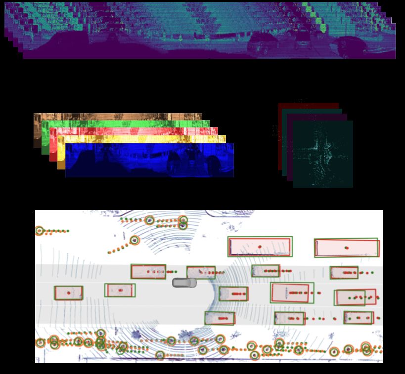
4.6. Qualitative Analysis
4.5. Run-time Analysis We present a qualitative comparison of our proposed
We report the run-time results using a Titan RTX GPU. multi-view model with a single-view BEV-only method, in
Our method can process the operating range of 50m on Figure 4. While detection of vehicles is similar between the
nuScenes in ∼ 30ms and the range of 100m on our inter- two methods, MVFusenet more accurately detects pedestri-
nal data set in ∼ 55ms. In contrast, the previous BEV-only ans. Also, we show a few cases where our method is able to
method [4] runs on the shorter range of 50m in ∼ 38ms [5]. improve the motion prediction of vehicles and pedestrians
7Figure 4: Qualitative comparison of proposed MVFusenet with the BEV-only model which uses BEV in both temporal fusion
and the backbone. Model outputs for detections and trajectories are depicted in red for vehicles and in orange for pedestrians.
The ground truth is depicted in green. In (a), the MVFusenet model produces better quality motion forecasts as compared
to the BEV-only method for a moving vehicle (middle left). In (b), the BEV-only method exhibits multiple failure modes
for pedestrians pertaining to a false positive (left), a false negative (top middle), and an inaccurate trajectory for the moving
pedestrian (top right), while MVFusenet exhibits the correct behavior. The example in (c) shows the BEV-only model failing
to detect a pedestrian adjacent to the vehicle. Finally, in (d) we see that both models fail to accurately predict the position at
3s for a vehicle turning sharply, but the proposed model more accurately predicts the turning behaviour.
over single-view BEV-only method. mance over only using BEV. Finally, we established a new
state-of-the-art result on the publicly available nuScenes
data set for joint detection and forecasting.
5. Conclusion and Future Work In addition, we have demonstrated that the pre-
We presented a novel multi-view model for end-to-end sented LiDAR-only approach outperforms multi-sensor ap-
object detection and motion forecasting. We introduced a proaches which rely on RADAR or camera. However, as
unique method for multi-view temporal fusion, as well as future work, we plan to incorporate these additional sen-
a novel multi-view backbone network. We proved the ef- sors to improve the robustness of the proposed approach.
fectiveness of our approach as compared to existing single- Additionally, we used a simple uncertainty representation
view and multi-view fusion methods on two large-scale and forecasting method to simplify the experimentation. In
data sets. We showed that the proposed method can lever- the future, we plan to incorporate recent advances in multi-
age the complementary information in the RV and BEV modal motion forecasting and actor-scene interactions.
and improve accuracy on both detection and motion fore-
casting tasks, while maintaining low latency and scaling
to larger operating ranges. In particular, we demonstrated
that incorporating both views in temporal fusion and using
a sequential fusion approach significantly improves perfor-
8References [13] Yin Zhou and Oncel Tuzel. VoxelNet: End-to-end learning
for point cloud based 3D object detection. In Proceedings of
[1] Sergio Casas, Cole Gulino, Renjie Liao, and Raquel Ur- the IEEE CVPR, 2018. 2
tasun. Spatially-aware graph neural networks for rela-
tional behavior forecasting from sensor data. arXiv preprint [14] Yan Yan, Yuxing Mao, and Bo Li. SECOND: Sparsely em-
arXiv:1910.08233, 2019. 1, 2, 5, 6 bedded convolutional detection. Sensors, 2018. 2
[2] Sergio Casas, Wenjie Luo, and Raquel Urtasun. Intent- [15] Bin Yang, Wenjie Luo, and Raquel Urtasun. PIXOR: Real-
Net: Learning to predict intention from raw sensor data. In time 3D object detection from point clouds. In Proceedings
Proceedings of the Conference on Robot Learning (CoRL), of the IEEE CVPR, 2018. 2
2018. 1, 2, 4, 5, 6
[16] Yang Zhang, Zixiang Zhou, Philip David, Xiangyu Yue, Ze-
[3] Ankit Laddha, Shivam Gautam, Gregory P Meyer, and Car- rong Xi, Boqing Gong, and Hassan Foroosh. Polarnet: An
los Vallespi-Gonzalez. Rv-fusenet: Range view based fusion improved grid representation for online lidar point clouds se-
of time-series lidar data for joint 3d object detection and mo- mantic segmentation. In Proceedings of the IEEE/CVF Con-
tion forecasting. arXiv preprint arXiv:2005.10863, 2020. 1, ference on Computer Vision and Pattern Recognition, pages
2, 4, 5, 6, 7 9601–9610, 2020. 2
[4] Nemanja Djuric, Henggang Cui, Zhaoen Su, Shangxuan
[17] Bo Li, Tianlei Zhang, and Tian Xia. Vehicle detection from
Wu, Huahua Wang, Fang-Chieh Chou, Luisa San Martin,
3d lidar using fully convolutional network. arXiv preprint
Song Feng, Rui Hu, Yang Xu, Alyssa Dayan, Sidney Zhang,
arXiv:1608.07916, 2016. 2
Brian C. Becker, Gregory P. Meyer, Carlos V-Gonzalez, and
Carl K. Wellington. Multixnet: Multiclass multistage multi- [18] Andres Milioto, Ignacio Vizzo, Jens Behley, and Cyrill
modal motion prediction, 2020. 1, 2, 4, 5, 6, 7 Stachniss. Rangenet++: Fast and accurate lidar semantic
[5] Meet Shah, Zhiling Huang, Ankit Laddha, Matthew Lang- segmentation. In 2019 IEEE/RSJ International Conference
ford, Blake Barber, Sidney Zhang, Carlos Vallespi-Gonzalez, on Intelligent Robots and Systems (IROS), pages 4213–4220.
and Raquel Urtasun. Liranet: End-to-end trajectory pre- IEEE, 2019. 2
diction using spatio-temporal radar fusion. arXiv preprint [19] Deyvid Kochanov, Fatemeh Karimi Nejadasl, and Olaf
arXiv:2010.00731, 2020. 1, 2, 5, 6, 7 Booij. Kprnet: Improving projection-based lidar semantic
[6] Gregory P Meyer, Jake Charland, Shreyash Pandey, Ankit segmentation. arXiv preprint arXiv:2007.12668, 2020. 2
Laddha, Carlos Vallespi-Gonzalez, and Carl K Wellington. [20] Xiaozhi Chen, Huimin Ma, Ji Wan, Bo Li, and Tian Xia.
Laserflow: Efficient and probabilistic object detection and Multi-view 3D object detection network for autonomous
motion forecasting. arXiv preprint arXiv:2003.05982, 2020. driving. In Proceedings of the IEEE CVPR, 2017. 2
1, 2, 4, 6, 7
[21] Yin Zhou, Pei Sun, Yu Zhang, Dragomir Anguelov, Jiyang
[7] Gregory P. Meyer, Ankit Laddha, Eric Kee, Carlos Vallespi-
Gao, Tom Ouyang, James Guo, Jiquan Ngiam, and Vijay Va-
Gonzalez, and Carl K. Wellington. LaserNet: An efficient
sudevan. End-to-end multi-view fusion for 3d object detec-
probabilistic 3D object detector for autonomous driving. In
tion in lidar point clouds. In Conference on Robot Learning,
Proceedings of the IEEE CVPR, 2019. 1, 2, 4
pages 923–932. PMLR, 2020. 2, 4
[8] Alex H. Lang, Sourabh Vora, Holger Caesar, Lubing Zhou,
Jiong Yang, and Oscar Beijbom. PointPillars: Fast encoders [22] Ke Chen, Ryan Oldja, Nikolai Smolyanskiy, Stan Birchfield,
for object detection from point clouds. In Proceedings of the Alexander Popov, David Wehr, Ibrahim Eden, and Joachim
IEEE CVPR, 2010. 2, 4 Pehserl. Mvlidarnet: Real-time multi-class scene under-
standing for autonomous driving using multiple views. arXiv
[9] Yin Zhou, Pei Sun, Yu Zhang, Dragomir Anguelov, Jiyang
preprint arXiv:2006.05518, 2020. 2
Gao, Tom Ouyang, James Guo, Jiquan Ngiam, and Vijay Va-
sudevan. End-to-end multi-view fusion for 3d object detec- [23] Venice Erin Liong, Thi Ngoc Tho Nguyen, Sergi Wid-
tion in lidar point clouds. In Conference on Robot Learning, jaja, Dhananjai Sharma, and Zhuang Jie Chong. Amvnet:
2020. 2 Assertion-based multi-view fusion network for lidar seman-
[10] Sudeep Fadadu, Shreyash Pandey, Darshan Hegde, Yi Shi, tic segmentation. arXiv preprint arXiv:2012.04934, 2020.
Fang-Chieh Chou, Nemanja Djuric, and Carlos Vallespi- 2
Gonzalez. Multi-view fusion of sensor data for improved [24] Zhidong Liang, Ming Zhang, Zehan Zhang, Xian Zhao, and
perception and prediction in autonomous driving. arXiv Shiliang Pu. Rangercnn: Towards fast and accurate 3d object
preprint arXiv:2008.11901, 2020. 2, 5, 6 detection with range image representation. arXiv preprint
[11] Shaoshuai Shi, Xiaogang Wang, and Hongsheng Li. PointR- arXiv:2009.00206, 2020. 2
CNN: 3D object proposal generation and detection from [25] Nemanja Djuric, Vladan Radosavljevic, Henggang Cui, Thi
point cloud. In Proceedings of the IEEE CVPR, 2019. 2 Nguyen, Fang-Chieh Chou, Tsung-Han Lin, and Jeff Schnei-
[12] Zetong Yang, Yanan Sun, Shu Liu, Xiaoyong Shen, and Jiaya der. Motion prediction of traffic actors for autonomous
Jia. STD: Sparse-to-dense 3D object detector for point cloud. driving using deep convolutional networks. arXiv preprint
In Proceedings of the IEEE ICCV, 2019. 2 arXiv:1808.05819, 2018. 2
9[26] Alexandre Alahi, Kratarth Goel, Vignesh Ramanathan, trajectory prediction. In European Conference on Computer
Alexandre Robicquet, Li Fei-Fei, and Silvio Savarese. So- Vision, pages 507–523. Springer, 2020. 2
cial LSTM: Human trajectory prediction in crowded spaces. [39] Agrim Gupta, Justin Johnson, Li Fei-Fei, Silvio Savarese,
In Proceedings of the IEEE CVPR, 2016. 2 and Alexandre Alahi. Social gan: Socially acceptable tra-
[27] Nachiket Deo and Mohan M Trivedi. Convolutional social jectories with generative adversarial networks. In Proceed-
pooling for vehicle trajectory prediction. In Proceedings of ings of the IEEE Conference on Computer Vision and Pattern
the IEEE CVPR Workshops (CVPRW), 2018. 2 Recognition, pages 2255–2264, 2018. 2
[28] Namhoon Lee, Wongun Choi, Paul Vernaza, Christopher B [40] Ming Liang, Bin Yang, Rui Hu, Yun Chen, Renjie Liao,
Choy, Philip HS Torr, and Manmohan Chandraker. DESIRE: Song Feng, and Raquel Urtasun. Learning lane graph
Distant future prediction in dynamic scenes with interacting representations for motion forecasting. arXiv preprint
agents. In Proceedings of the IEEE CVPR, 2017. 2 arXiv:2007.13732, 2020. 2
[29] Gregory P. Meyer, Jake Charland, Darshan Hegde, Ankit [41] Wenjie Luo, Bin Yang, and Raquel Urtasun. Fast and furi-
Laddha, and Carlos Vallespi-Gonzalez. Sensor fusion for ous: Real time end-to-end 3D detection, tracking and motion
joint 3D object detection and semantic segmentation. In Pro- forecasting with a single convolutional net. In Proceedings
ceedings of the IEEE CVPR Workshops (CVPRW), 2019. 2 of the IEEE CVPR, 2018. 2
[30] Karttikeya Mangalam, Harshayu Girase, Shreyas Agarwal, [42] Kaiming He, Xiangyu Zhang, Shaoqing Ren, and Jian Sun.
Kuan-Hui Lee, Ehsan Adeli, Jitendra Malik, and Adrien Deep residual learning for image recognition. In Proceedings
Gaidon. It is not the journey but the destination: End- of the IEEE CVPR, 2016. 4
point conditioned trajectory prediction. arXiv preprint [43] Tianwei Yin, Xingyi Zhou, and Philipp Krähenbühl. Center-
arXiv:2004.02025, 2020. 2 based 3d object detection and tracking. arXiv preprint
[31] Hang Zhao, Jiyang Gao, Tian Lan, Chen Sun, Benjamin arXiv:2006.11275, 2020. 5
Sapp, Balakrishnan Varadarajan, Yue Shen, Yi Shen, Yuning [44] Tsung-Yi Lin, Priya Goyal, Ross Girshick, Kaiming He, and
Chai, Cordelia Schmid, et al. Tnt: Target-driven trajectory Piotr Dollár. Focal loss for dense object detection. In Pro-
prediction. arXiv preprint arXiv:2008.08294, 2020. 2 ceedings of the IEEE ICCV, 2017. 5
[32] Yuning Chai, Benjamin Sapp, Mayank Bansal, and Dragomir [45] Gregory P Meyer and Niranjan Thakurdesai. Learning an
Anguelov. MultiPath: Multiple probabilistic anchor tra- uncertainty-aware object detector for autonomous driving.
jectory hypotheses for behavior prediction. arXiv preprint arXiv preprint arXiv:1910.11375, 2019. 5
arXiv:1910.05449, 2019. 2
[46] Holger Caesar, Varun Bankiti, Alex H Lang, Sourabh Vora,
[33] Tung Phan-Minh, Elena Corina Grigore, Freddy A Boulton, Venice Erin Liong, Qiang Xu, Anush Krishnan, Yu Pan, Gi-
Oscar Beijbom, and Eric M Wolff. Covernet: Multimodal ancarlo Baldan, and Oscar Beijbom. NuScenes: A mul-
behavior prediction using trajectory sets. In Proceedings of timodal dataset for autonomous driving. arXiv preprint
the IEEE CVPR, 2020. 2 arXiv:1903.11027, 2019. 5
[34] Nicholas Rhinehart, Rowan McAllister, Kris Kitani, and [47] Adam Paszke, Sam Gross, Francisco Massa, Adam Lerer,
Sergey Levine. Precog: Prediction conditioned on goals in James Bradbury, Gregory Chanan, Trevor Killeen, Zeming
visual multi-agent settings. In Proceedings of the IEEE/CVF Lin, Natalia Gimelshein, Luca Antiga, et al. Pytorch: An im-
International Conference on Computer Vision, pages 2821– perative style, high-performance deep learning library. arXiv
2830, 2019. 2 preprint arXiv:1912.01703, 2019. 5
[35] Charlie Tang and Russ R Salakhutdinov. Multiple futures
prediction. In Proceedings of Advances in Neural Informa-
tion Processing Systems (NIPS), 2019. 2
[36] Henggang Cui, Vladan Radosavljevic, Fang-Chieh Chou,
Tsung-Han Lin, Thi Nguyen, Tzu-Kuo Huang, Jeff Schnei-
der, and Nemanja Djuric. Multimodal trajectory predictions
for autonomous driving using deep convolutional networks.
In 2019 International Conference on Robotics and Automa-
tion (ICRA). IEEE, 2019. 2
[37] Jiyang Gao, Chen Sun, Hang Zhao, Yi Shen, Dragomir
Anguelov, Congcong Li, and Cordelia Schmid. Vectornet:
Encoding hd maps and agent dynamics from vectorized rep-
resentation. In Proceedings of the IEEE/CVF Conference
on Computer Vision and Pattern Recognition, pages 11525–
11533, 2020. 2
[38] Cunjun Yu, Xiao Ma, Jiawei Ren, Haiyu Zhao, and Shuai Yi.
Spatio-temporal graph transformer networks for pedestrian
10You can also read