A TDOA-based multiple source localization using delay density maps
←
→
Page content transcription
If your browser does not render page correctly, please read the page content below
Sådhanå (2020)45:204                                                                                                          Indian Academy of Sciences
https://doi.org/10.1007/s12046-020-01453-8
                                         Sadhana(0123456789().,-volV)FT3](012345
                                                                             6789().,-volV)

A TDOA-based multiple source localization using delay density maps
           RITU BOORA*           and SANJEEV KUMAR DHULL

           Guru Jambheshwar University of Science and Technology, Hisar 125001, India
           e-mail: rituboora@gmail.com; sanjeevdhull2011@yahoo.com

           MS received 8 April 2020; revised 21 June 2020; accepted 5 July 2020

           Abstract. The higher computational efficiency of the time difference of arrival (TDOA) based sound source
           localization makes it a preferred choice over steered response power (SRP) methods in real-time applications.
           However, unlike SRP, its implementation for multiple source localization (MSL) is not straight forward. It
           includes challenges as accurate feature extraction in unfavourable acoustic conditions, association ambiguity
           involved in mapping the feature extractions to the corresponding sources and complexity involved in solving the
           hyperbolic delay equation to estimate the source coordinates. Moreover, the dominating source and early
           reverberation make the detection of delay associated with the submissive sources further perplexing. Hence, this
           paper proposes a proficient three-step method for localizing multiple sources from delay estimates. In step 1, the
           search space region is partitioned into cubic subvolumes, and the delay bound associated with each one is
           computed. Hereafter, these subvolumes are grouped differently, such that whose associated TDOA bounds are
           enclosed by a specific delay interval, are clustered together. In step 2, initially, the delay segments and later each
           subvolume contained by the corresponding delay segment are traced for passing through estimated delay
           hyperbola. These traced volumes are updated by the weight to measure the likelihood of a source in it. The
           resultant generates the delay density map in the search space. In the final step, localization enhancement is
           carried out in the selected volumes using conventional SRP (C-SRP). The validation of the proposed approach is
           done by carrying out the experiments under different acoustic conditions on the synthesized data and, recordings
           from SMARD & Audio Visual 16.3 Corpus.

           Keywords. Sensor arrays; acoustic signal processing; time difference of arrival (TDOA); multiple source
           localization; steered response power-phase transform (SRP-PHAT); generalized cross-correlation (GCC).

1. Introduction                                                                               mathematical manipulation. The key to the effectiveness of
                                                                                              these localizers is an accurate and robust TDOA estimators
The localization of an acoustic event is the fundamental                                      and hence, to overcome this issue, several mathematical
prerequisite for developing applications such as human-                                       procedures like Adaptive Eigen Value Decomposition
machine interaction, robotics, videoconferencing, hands-                                      (AED) [5], GCC-PHAT [6], a geometric approach using
free communication, military surveillance, acoustic scene                                     non-coplanar arrays [7], a modified version of Maximum
analysis, hearing aids, smart environments and many more.                                     Likelihood [8], a combination of linear interpolation and
With the growing demand for the proficient methods of                                          Cross-Correlation (CC) [9], etc. have been adopted.
sound source localization (SSL), many efforts have been                                       Amongst these, GCC-PHAT is the most widely used
devoted by researchers to examine this field and develop                                       method to estimate TDOA as it is conceptually simple
several methodologies to solve this central problem of                                        [10–12]. As shown in figure 1, each TDOA measurement in
signal processing. Amongst the existing methods, those                                        the realizable delay interval [-D/v, D/v] (where D is inter
based on TDOA are fast, but their performance deteriorates                                    sensor distance and v is the velocity in medium) of a sensor
in challenging conditions. Hence, there is continuous effort                                  pair corresponds to a distinct half hyperbolic branch in 2-D
to make them robust and computationally simple [1–4].                                         with sensor locations as its foci’s. The estimated source
   TDOA based techniques involve a 2-step procedure                                           position is the intersection point of the hyperbolic branches
wherein initially the received signal at the sensor array is                                  corresponding to estimated TDOA at different sensor pairs.
processed to compute the TDOA between the microphone                                          However, solving the nonlinear hyperbolic complex and
pairs. Thereafter the estimated delay for each sensor pair is                                 moreover, the solution becomes inconsistent with inaccu-
mapped to the corresponding source positions by some                                          racies in TDOA measurements. Henceforth, researchers are
                                                                                              continuously involved to suggest numerous approaches to
                                                                                              solve these hyperbolic equations which include planar
*For correspondence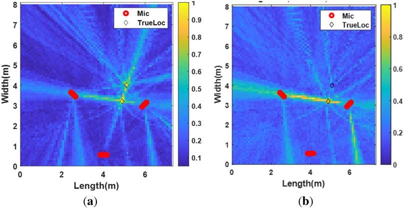
204   Page 2 of 12                                                                      Sådhanå (2020)45:204

                                                                  Figure 2. Two hyperbolas from each sensor pair (black dots) in
Figure 1. Confocal hyperbolas for a range of physically realiz-   respect of two sources (purple dots).
able TDOAs’ of a sensor pair.

intersection (PI), spherical intersections (SX), spherical            parameters, one source may supersede other sources.
interpolation (SI) [13], least square and weighted least              The work in [17] has ascertained the relationship
square (WLS), global branch and bound [14], space-range               between the correlation values and source character-
reference frames [15], WLS with cone tangent plain con-               istics. The submissive sources show less coherence at
strain [16], etc.                                                     most of the microphone pairs, and thus, it is overtaken
                                                                      by early reverberations more often. As a result, the
                                                                      GCC values at these secondary peaks might not
1.1 Challenges in TDOA based multiple source                          provide the correct likelihood of a source.
                                                                    • Spatial resolution: The two sources may become
localization (MSL)
                                                                      indistinguishable when narrowly positioned in the
In a realistic scenario, there are often situations where             lower sensitive area. It can be analysed from figure 1,
multiple sources are simultaneously active, and there is a            where the sensor pair shows varying spatial sensitivity
need to localize them simultaneously. Several authors have            in the search space. The subregion B, when compared
proposed different methods based on Steered Response                  to subregion A, has lower spatial sensitivity as it has
Power (SRP) and Time Difference of Arrival (TDOA) to                  only a very few and widely spaced hyperbolas passing
localize multiple sources; some of these are discussed in the         through it. Thus, two narrowly separated sources in the
literature section. However, unlike SRP, none of the                  subregion B may show the same delay to the sensor
existing TDOA based localization methods can be directly              pair and therefore become indistinguishable.
extended to multiple sources due to several challenges
                                                                  A proficient TDOA based method to overcome the above-
discussed below.
                                                                  said ambiguities is proposed in the paper. However, before
  • Multi-source ambiguity: In an acoustic setup with             proceeding with the proposed method, the related literature
    K sources (K [ 1), it is generally expected that each         and their significant contributions are discussed below. The
    sensor pair GCC will contain at least K local extrema,        remaining part of the paper is delivered as follows. The
    corresponding to each source. Identifying the correct         literature on multiple source localization is elaborated in
    TDOA estimate and matching to the corresponding               section 2. Section 3 introduces the proposed method and,
    source is a big challenge called multi-source ambigu-         the results and discussion are presented in section 4. Con-
    ity. As displayed in figure 2, the hyperbolas corre-           clusions are provided in section 5.
    sponding to the estimated delays of both the sources at
    each sensor pair gives four intersections, where only
    two corresponds to the true source and remaining are          2. Literature on multiple source localization
    the phantom sources. Subsequently, it gets complicated
    to differentiate the correct locations from the phantom
                                                                  2.1 TDOA based
    sources. Furthermore, the TDOA mapping becomes
    more problematic with reverberation when the indirect         TDOA based clustering method [18] suggests a three stage
    path GCC peak of a source is higher than that of its          strategy which includes pre-whitening the signal, comput-
    direct path.                                                  ing the TDOA of the direct path and early reflections by the
  • Dominant source: In a multi-sourced environment, due          time delay estimation method and, clustering the hyperbolic
    to different frequency spectrum or propagation                intersection while rejecting the outliers. The intersection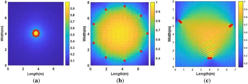
Sådhanå (2020)45:204                                                                    Page 3 of 12     204

points calculated from all the permutation of the estimated       active regions. It consequently restricts the usage of
TDOAs are clustered based on some criteria. The centre of         competent methods to solve the hyperbolic equations and
each cluster is then considered as the estimated source           hence affects the accuracy within the active sector. It is also
location. Later, a few variants of clustering algorithm as        demonstrated in figure 3, where a source placed at coor-
short clustering for moving speakers [19], K-means??              dinates (1, 5) is localized at (1.7, 4.8). Moreover, this
[20], competitive K-means [21], multi-path matching pur-          detection of IDIR with the single active region is compu-
suit [10] were also explored. However, these algorithm            tationally expensive.
results in voluminous permutations of clusters in a rever-
berant environment which subsequently tempts to phantom
source locations. Authors in work [22–24] suggested solu-         2.2 SRP based
tion based on consistent graph along with filters like raster
                                                                  The beam steering methods are very robust but, evaluating
condition, Zero-sum condition, upper bound on TDOA etc.
                                                                  the objective functions at all the candidate locations is quite
to eliminate the undesirable TDOA. However, the cum-
bersome process involved in implementing the graphs               cumbersome and subsequently limits their practical
limits their applicability. Work in [25] uses multiple            deployment. To accelerate SRP based localization, the
hypothesis frameworks for TDOA disambiguation, but its            work in [26–28] offers hierarchical search procedure for
performance degrades with reverberations.                         coarse to fine identification of potential source locations.
                                                                  However, they tend to miss the source locations before the
   A hybrid method based on TDOA and SRP is introduced
                                                                  final stage as after each iteration they prune the candidate
in work [12] where a spatial enclosure is partitioned into
                                                                  source locations with lesser probability.
several elemental regions such that each partition contains
                                                                     Work presented in [29] manipulates the GCC-PHAT
at most one source. The characteristics delay interval
associated with each elemental region maps to an area             measurements to extract the information of submissive
circumscribed by the pair of hyperboloid branches called          sources. In this method, the dominating speaker location is
Inverse Delay Interval Region (IDIR) or characteristic            deduced straightforwardly by maximizing the Global
IDIR. However, the foremost challenge here is to decide the       Coherence Field (GCF) acoustic map. Further, the domi-
                                                                  nant source is de-emphasized by reducing the magnitude of
shape of the elemental region such that it contains at most
                                                                  the GCC at delays associated with its locations. The GCF
one source and approximates the intersection of IDIR of all
                                                                  acoustic map is re-computed from de-emphasized GCC to
the sensor pairs. The factors like unequal characteristics
                                                                  extract the information of the submissive source. Hence,
intervals associated with each partition, reverberations,
additive noise, etc., adversely affect in estimating the          this method is referred by Global Coherence Field De-
accurate active region. It is illustrated in figure 3, where a     emphasized (GCF-D) for convenience in further text.
source placed at (1.5, 3.3) is erratically estimated in another   However, the prime challenge here is to design the opti-
elemental region at (3.1, 7.3). Further, for TDOA disam-          mum de-emphasizing function, which accentuates the GCC
                                                                  at desired delays without affecting the remaining. As
biguation, the delay information is discarded from the
                                                                  illustrated, the inappropriate de-emphasization of the
sensors pairs whose characteristics IDIR contain multiple
                                                                  dominating source shifts the second peak of the GCF
                                                                  acoustic map from the location (4.9, 3.2) in figure 4a to
                                                                  (4.2, 3.5) in figure 4b. Furthermore, a narrow de-emphasis
                                                                  filter may also not remove the relevant GCC effectively and
                                                                  adversely affect the performance of the method. Besides
                                                                  this, the acoustic map is to be computed times’ the number
                                                                  of sources present and hence, demands high computations
                                                                  and necessitates source prior information. However, none
                                                                  of the current methods has achieved the desired charac-
                                                                  teristics to meet the growing demand in numerous
                                                                  applications.

                                                                  3. Proposed method

                                                                  In the proposed method, initially, the search region is
                                                                  divided into cubic subvolumes, and the associated delay
                                                                  bound with each one is computed. Hereafter, the physically
                                                                  realizable delay interval of each sensor pair is segmented
                                                                  into small intervals and, the subvolumes are assembled in a
Figure 3. Active sector and fine localization error using IDIR.    way that whose associated delay bound lies in a segmented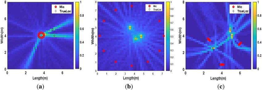
204   Page 4 of 12                                                                             Sådhanå (2020)45:204

                                 Figure 4. GCF map (a) Prior to De-emphasis. (b) After GCC De-emphasis.


interval are clustered together. Following this, the delay           characterized as         sp;max ; sp;max þ 1; . . .; 1; 0; 1; . . .;
segments through which estimated delay hyperbola of the              sp;max  1; sp;max g with sp,max = round(fs * D/v). The neg-
corresponding sensor pair passes are identified. The vol-             ative delay means that the source is closer to the sensor p1
umes contained by these delay segments are scanned and               than p2 of pth pair while a positive delay means a vice-
updated by weight only if the estimated delay hyperbola              versa. Consequently, the delay measured between any two
passes through them. When executed for all the sensor                microphones signals using GCC-PHAT is restricted by the
pairs, it provides the likelihood of a source in any volume.         delay interval [- sp,max, sp,max] to eliminate the undesired
Towards the end, the localization refinement is performed             computations [11].
using C-SRP in the subvolumes that are more likely to                   The coherence, wp[s] between the two received signals,
contain the source. The proposed method is detailed in the           sp1(t) and sp2(t) at pth sensor pair is computed using Eq. (3)
following subsections.                                               with Sp1, Sp2 as their respective N point Discrete Fourier
                                                                     Transform (DFT) where * represents a complex conjugate.
                                                                     The estimated relative delay sbp , evaluated by Eq. (4) for pth
3.1 TDOA estimation                                                  sensor pair is the value of s that maximizes the normalized
The received signal, si ðtÞ at ith sensor and at instant t in a      coherence function wp ½s [6].
multi-path and multi-source environment of K sources can
                                                                                                X1
                                                                                               NDFT
                                                                                                       Sp1 ½mSp2 ½m j 2psm
be modelled using Eq. (1) where xk(t) is the kth source                             wp ½s ¼                            e NDFT          ð3Þ
signal transmitted, hk,i(t) is impulse response from kth                                       m¼0
                                                                                                      jSp1 ½mSp2 ½mj
source to ith sensor, and N i ðtÞ is Additive White Gaussian
Noise (AWGN).                                                                              sbp ¼ arg max wp ½s                         ð4Þ
                                                                                                 |fflfflfflffl{zfflfflfflffl}
                                                                                                  s2½smax ;smax
                          X
                          K
              si ðt Þ ¼         hk;i ðtÞ  xk ðtÞ þ N i ðtÞ    ð1Þ
                          k¼1

From a set of M sensors, the P different sensors pair are            3.2 Constant and distinct delay hyperbolas
constituted as M(M - 1)/2. The TDOA (in samples) asso-               in the search space
ciated with a source placed at X(x, y, z) and the two sensors
of pth pair positioned at Xp1, Xp2 respectively, is evaluated        The relative delay is given in Eq. (2) and maps any point
from Eq. (2) where fs is the sampling frequency and v is the         X from the spatial search space to 1-D TDOA vector. Pres-
propagation speed of the signal.                                     ence of several locations with similar TDOA on a half
                                                                     hyperboloid branch with foci at two microphones, it is

     sp ð X Þ ¼ round Xp1  X jjjjXp2  X =v  fs    ð2Þ        inferred that this mapping is not unique. This geometrical
                                                                     interpretation of a constant TDOA to a hyperboloid provides
The set of physically attainable delay for any sensor pair is        the locus of the possible source location. The relative delay is
bounded by the distance, D between the sensor pair and is            continuous in X, and henceforth, the source locations with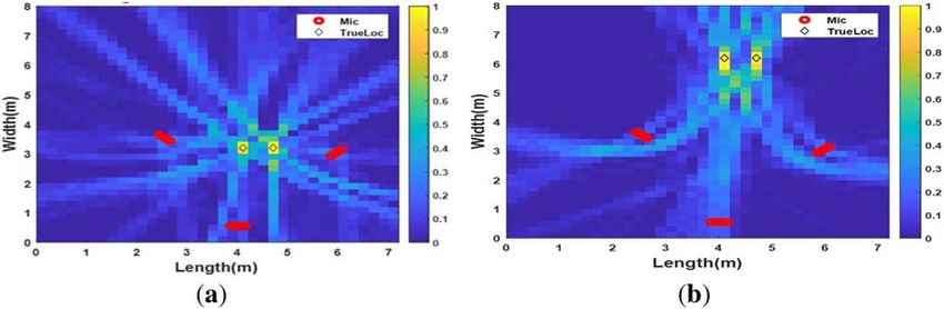
Sådhanå (2020)45:204 Page 5 of 12 204
different TDOA will lead to distinct and confocal half boundary surface of this given search volume [31], the
hyperboloid branches, as shown in figure 1, for 2-D. minimum and maximum delay comes out to be sVmin ¼
min sp ðX 2 oVÞ and sVmax ¼ max sp ðX 2 oVÞ respectively.
X2V X2V
3.3 Delay bound associated with a cubic volume Using this, we compute the Delay Density Map of the entire
search region.
The TDOA associated with a volume can take values only in a Therefore, an estimated kth delay, skp from the GCC of
range defined by its boundary surface. Therefore, the delay
the pth sensor pair is mapped to a subvolume Vsub only if it
bounds related to a volume can be calculated from the maxi-
mum and minimum TDOA values on its boundary surface. is contained by its associated TDOA bound, ½sVp;min
sub
; sVp;max
sub
.
However, for the accurate associated TDOA range measure- Furthermore, only the subvolumes which are mapped by
ment, it requires computing the TDOA on a dense grid on all the estimated delay in the search space are updated by a
the bounding surfaces of the volume, making it computa- unity weight. It is mathematically represented by Eq. (10).
tionally expensive [30]. Therefore, in this paper, a gradient- Henceforth, the objective function for each volume,
based approach [31] has been followed that is equally efficient W(Vsub) is evaluated from Eq. (11), which involves sum-
and involves a much lesser number of computations. ming the projections of Eq. (10) for the K delays over the
Initially, a given search volume V P that contains the comprehensive P set of sensor pairs. When computed across
source(s) is segmented into a set of uniform cubic all the Vsub 2 , it represents the density of passing
subvolumes, Vsub. These subvolumes are created such that through estimated delay hyperbolas through each and hence
each grid point of a uniform spatial grid in the search space named delay density map (DDM). Thus, the DDM displays
defines the center of a subvolume. The associated boundary the likelihood of a source in each subvolume.
to each subvolume is the symmetrical region of half the 1; for sVp;min
sub
skp sVp;max
sub
grid resolution around each point. vp sk ; Vsub ¼ ð10Þ
Next, the direction of the maximum increase of delay at
each grid point is calculated by the gradient function, given P X
X K
in Eq. (5). The gradient in the individual direction (x, y and W ðVsub Þ ¼ sp sk ; Vsub ð11Þ
z) is computed by Eq. (6) where c 2 ðx; y; or zÞ [31]. p¼1 k¼1
rsp ð X Þ ¼ rx sp ð X Þ; ry sp ð X Þ; rz sp ð X Þ ð5Þ Assigning equal weights to the mapped subvolumes for
! each K number of GCC peaks benefits to recover the
osp ð X Þ 1 c cp1 c cp2 sources with small coherence values. Moreover, it helps to
rc sp ðXÞ ¼ ¼ ð6Þ
oc c X Xp1 X Xp2 suppress the early reverberation with large GCC peak val-
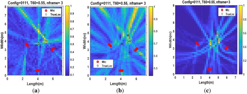
ues. It is demonstrated with the help of figure 5, which
Thereafter, the TDOA bounds for a symmetrical subvolume displays the localization of three sources in a frame for
Vsub surrounding a grid location are calculated from Eq. (7) various techniques when RT60 is 0.55 sec. In figure 5a and
and Eq. (8) where d, defined in Eq. (9) is the distance from b, the acoustic map of the search region is developed using
the center to the boundary of Vsub and r is the grid size (i.e., C-SRP and Mean Modified SRP (MMSRP) [32] respec-
is the distance between the centers of two adjacent Vsub). tively while figure 5c displays the delay density map. From
figure 5a and b, it is observed that each acoustic map has
sVp;min
sub
¼ sp ð X Þ rsp ð X Þ d ð7Þ many high SRP points at locations other than the source and
hence couldn’t localize all the three sources. In contrast,
sVp;max
sub
¼ sp ð X Þ þ rsp ð X Þ d ð8Þ figure 5c shows the high likelihood only in the regions that
contain the source.
r 1 1 1
d ¼ min ; ; ð9Þ
2 jsinhcos/j jsinhsin/j jcoshj
3.5 Computing DDM using subvolume clustering
Where h ¼ cos 1 rz sp ðX Þ
and P
jjrsp ðX Þjj Up to now, each Vsub 2 in the enclosure needs to be
/ ¼ atan2 ðry sp ðXÞ; rx sp ðXÞÞ. scanned for mapping an estimated TDOA to a respective
Vsub and therefore, it is a computationally expensive pro-
cess. Hence, this section introduces a delay segmentation
3.4 Delay density maps and subvolume clustering approach to minimize the DDM
computational expense.
By definition of associated TDOA to a volume, for any 3.5a Delay segmentation: As discussed, the distinct
source located in volume V in the search space, the TDOA TDOA to spatial mapping appears as continuous confocal
at a sensor pair for this source also lies in a range, tightly half hyperboloid branches when the delay is traversed from
bounded by the two hyperboloid branches. With oV as the sp;max to sp,max for a sensor pair p. Consequently, a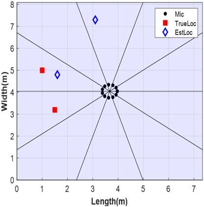
204    Page 6 of 12                                                                             Sådhanå (2020)45:204

         Figure 5. (a) Acoustic map using C-SRP. (b) Acoustic map using MMSRP. (c) DDM using the proposed method.

segmented delay interval [Ip,min: Ip,max] ( [-sp,max: sp,max]             mathematically represented by Eq. (13) where t 2
is mapped to a region bounded by two half hyperboloids                   ½P1; 2; . .P
                                                                                    .; T ; i.e. the tth delay interval. In this equation,
hp(Ip,min) and hp(Ip,max) corresponding to Ip,min and Ip,max                  /         - Vsub removes
                                                                                                   P       a subvolume from the complete
respectively. Henceforth, the entire range of realizable                  set of subvolumes          once it becomes a part of any cluster.
delay for a sensor pair is segmented into T intervals, as                 This step ensures that each group Gtp has unique elements
given in Eq. (12). As illustrated in figure 6, each region                 where Gtp is the tth group for the pth sensor pair.
corresponds to a segmented delay interval and therefore has                               X
hyperbolic spatial boundaries.                                                8Vsub 2         ; Gtp   Gtp [ Vsub and
                                                                                      X         X                                     ð13Þ
                                                                                                    Vsub if Ip;min
                                                                                                               t
                                                                                                                    \sVp;max
                                                                                                                        sub
                                                                                                                              Ip;max
                                                                                                                                t
½sp;max : sp;max $½Ip;min
                      1
                            : Ip;max
                               1
                                     [ Ip;min
                                        2
                                              : Ip;max
                                                 2
                                                       [    Ip;min
                                                                T

                     : Ip;max
                        T
                                                                 ð12Þ       3.5c Redefining the lower bound for each delay segment:
                                                                         In the previous subsection, the elements of a group Gtp have
  3.5b Subvolume clustering as per delay segmentation:                   been clustered considering only their upper TDOA bound
All the search space subvolumes are grouped such that                    sVp;max
                                                                            sub
                                                                                 . However, since each Vsub has its own lower delay
their respective upper TDOA bound, sVp;max sub
                                                lying in one             bound, sVp;min
                                                                                   sub
                                                                                        and it may overlap with the delay interval of
                 t       t
delay interval [Ip,min: Ip,max] are clustered together. It is            the previous segment (t - 1). It necessitates redefining the
                                                                         lower TDOA bound of each segment exclusively such that
                                                                         lower bound of the clustered volumes is also considered, as
                                                                         given in Eq. (14). The Eq. (13) and Eq. (14) collectively
                                                                         guarantee that there remains no Vsub which is not part of
                                                                         any cluster and no subvolume is mapped more than once for
                                                                         an estimated TDOA.

                                                                                t
                                                                               Ip;min ¼ min min sVp;min
                                                                                                   sub
                                                                                                        ; Ip;min
                                                                                                           t
                                                                                                                 8Vsub 2 Gtp          ð14Þ

                                                                            3.5d Delay density maps: Hereafter, for each sensor pair,
                                                                         initially, the delay segments and later the volume in this
                                                                         delay segments are traced for passing through correspond-
                                                                         ing estimated delay hyperbola. These traced Vsub are
                                                                         updated by a weight using Eq. (11) to measure the likeli-
                                                                         hood of a source in it. This whole process
                                                                                                                  P minimises the
                                                                         required TDOA mapping from the set           to a subset of
Figure 6. Delay segmentation and corresponding hyperbolas of             subvolumes contained by the traced delay segments. It thus
a sensor pair.                                                           makes the DDM computationally inexpensive.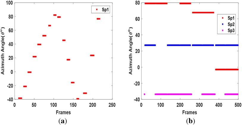
Sådhanå (2020)45:204                                                                 Page 7 of 12    204

3.6 Refined position estimation                                  evaluating the DDM on a coarse grid of 0.2 m, this
                                                                minimum distance is only 0.4 m and hence can come across
In the end, the refined position is evaluated in the K higher    the practical requirements. Thus, the spatial resolution of
likelihood selected subvolumes using C-SRP [11]. The            the proposed method is much higher than that of IDIR,
source location, Xk in kth sub-volume Vksub is estimated        where it is limited by the size of its elemental region.
using Eq. (15).                                                 Moreover, this resolution can be improved further by
                                  XP                          evaluating the DDM on a denser grid with a marginal
                Xk ¼ argmax           w sp ð X Þ        ð15Þ    compromise in the computational cost.
                     |fflfflfflffl{zfflfflfflffl} p¼1
                           k
                        X2Vsub
                                                                   The performance of the proposed method is evaluated
                                                                and compared with the 2-D state-of-art methods, IDIR [12]
                                                                and GCF-D [39] under various simulated acoustic settings.
                                                                The proposed method (Prop) and GCF-D have been simu-
4. Results and discussions                                      lated on DLA and large UCA. At the same time, IDIR is
                                                                limited to DLA configuration for competitive comparison
In this section, the proposed method is evaluated on various    as it yields poor results with L-UCA. It is mainly due to
simulated acoustic settings, SMARD database and AV16.3          inappropriate intersections of characteristics IDIR with
corpus.                                                         sectored elemental regions for large UCA. The methods are
                                                                simulated for localization with a sampling frequency of
                                                                44.1 KHz, frame length of 4096 samples with 50% overlap
                                                                and tested for 200 trials over random source locations. The
                                                                proposed method is implemented with the initial grid res-
4.1 Performance evaluation on simulated data
                                                                olution of 0.2 m to compute DDM and a final grid reso-
The simulated dataset is generated using Image method           lution of 0.01 m in the selected K regions. The GCF-D is
[33, 34] in a room of dimensions ½7:34 m  8:01 m              computed with a grid resolution of 0.01 m whereas IDIR is
2:87 m for various speech and music signals from TSP           implemented with 20 elemental regions in the form of
speech database [35] and MIS database respectively [36].        sectors.
   Before considering an array configuration, its spatial           Table 1 presents the Root Mean Square Error (RMSE) in
sensitivity was examined using Geometrically Sampled            the localization of the two sources separately under dif-
Grid procedure [37], as shown in figure 7. Each array            ferent RT60 (sec). As observed from these results, the
configuration has nine sensors which are equally spaced for      dominating source is localized with lower error with all the
small UCA and Large-UCA (L-UCA) of figures 7a and b,             methods. However, the proposed method shows a consid-
respectively. Whereas, the Distributed Linear Array (DLA)       erable improvement in the localization of the submissive
in figure 7c has three linear arrays with equally distributed    source and a slower degradation to reverberation as com-
sensors. As the physically realizable delay interval expands    pared to other methods. The array geometry is another
with an increase in the inter-sensor distance; the number of    critical factor which impacts the performance of these
hyperbolas passing through the region intensifies and            methods. The source localization performance of the pro-
improves the spatial resolution [38]. It explains the           posed method and GCF-D are superior with large UCA
enhanced sensitivity of Large-UCA over small UCA and            when compared to that of DLA, being enhanced spatial
DLA (cf. figure 7).                                              resolution provided by the earlier. Table 2 presents the
   Furthermore, the delay density maps of the search region     averaged RMSE over the number of sources present for
are developed using Eq. (11) for small UCA, L-UCA and           different reverberant settings. As clearly shown by these
DLA, respectively in figure 8a, b and c. As observed, the        results, the proposed method shows superior localization
three sources are accurately localized with DLA and             results for the multiple sources, whereas GCF-D is highly
L-UCA while small UCA shows comparatively higher                influenced by it.
delay density only in the source direction. Henceforth, the        The robustness to uncorrelated noise is evaluated by
performance of the proposed method for spatial localization     adding White Gaussian Noise (WGN) to each received
is evaluated using DLA and L-UCA array configuration.            microphone signal to achieve different SNR. Performance
   Moreover, as exhibited in figure 9, the spatial sensitivity   comparison of the proposed method with existing methods
of a sensor array configuration also impacts the minimum         is presented in figure 10 for a range of SNR.
resolvable distance between the two sources. The two               Noticeably, the proposed method shows the enhanced
sources show the relative spread of the peak in the delay       results over the state-of-art methods. Tables 1, 2 and fig-
density map (DDM) when placed in the lower sensitive area       ure 10 together validate the competency of the proposed
as in figure 9b in comparison to figure 9a. Hence, consid-        method in adverse acoustic conditions over the existing
ering the spread of the peaks to the neighbouring subvol-       methods.
umes, the two sources should be kept set apart by at least         4.1a Computational cost: Table 3 displays the compar-
twice the grid resolution for efficient localization. While      ison of the execution time (in sec) to localize the two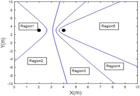
204    Page 8 of 12                                                                         Sådhanå (2020)45:204

Figure 7. Analysing the spatial sensitivity of different sensor array geometries. (a) Small UCA, (b) Large UCA and (c) Distributed
Linear Array (DLA).

Figure 8. Delay density map with different geometries (M = 12) for RT60 of 0.5 sec. (a) Small UCA, (b) Large-UCA and
(c) Distributed Linear Array.

      Figure 9. DDM in the different sensitive regions. (a) Higher sensitive region. (b) A comparatively lower sensitive region.

sources using a single frame of length 1 sec for the                   As shown, the GCF-D technique has the highest run-time
discussed methods. The methods are simulated in                     as it involves computing the SRP twice (as there are two
MATLAB and run on a system with Intel Core i5 processor             sources) on a fine grid and removal of the dominating peak
(1.99 GHz) and 8 GB RAM.                                            from GCC of each sensor pair before re-computing the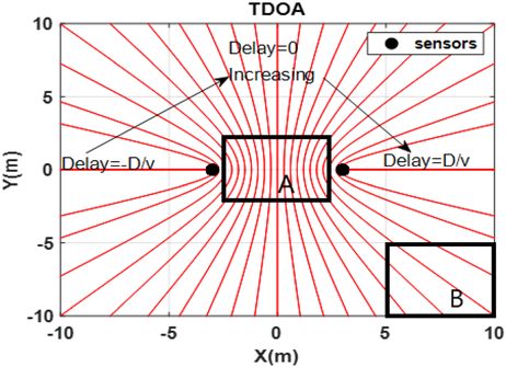
Sådhanå (2020)45:204                                                                        Page 9 of 12    204

Table 1. RMSE (m) in localization shown distinctly for the two sources (Src1, Src2) at different RT60 and SNR = 25 dB.

                               RT60 = 0.11 (sec)                    RT60 = 0.33 (sec)                         RT60 = 0.55 (sec)

Technique                   Src1               Src2              Src1               Src2                   Src1                   Src2
IDIR(DLA)                   0.16               0.38              0.20               0.51                   0.31                   0.82
GCF-D(DLA)                  0.21               0.61              0.32               0.82                   0.55                   1.01
Prop (DLA)                  0.12               0.17              0.15               0.21                   0.20                   0.29
GCF-D(UCA-D)                0.15               0.44              0.26               0.76                   0.41                   0.94
Prop(UCA-D)                 0.09               0.12              0.12               0.18                   0.17                   0.24

Table 2. RMSE in localization averaged over the number of active sources at various RT60 settings and SNR = 20 dB.

                                         RT60 = 0.33 sec                                              RT60 = 0.55 sec

                                     Number of active sources                                     Number of active sources

Technique                     1                    2               3                    1                    2                     3
IDIR(DLA)                    0.11              0.38               0.61              0.21                    0.56                  1.12
GCF-D(DLA)                   0.13              0.62               1.21              0.28                    0.82                  1.42
Prop (DLA)                   0.08              0.21               0.38              0.16                    0.27                  0.55
GCF-D(UCA-D)                 0.11              0.57               1.01              0.24                    0.72                  1.22
Prop(UCA-D)                  0.06              0.19               0.29              0.12                    0.24                  0.42

                                                                 Table 3. Execution time (sec) to localize the two sources (Src1,
                                                                 Src2) in a frame of 1 sec using DLA.

                                                                                                                     Techniques

                                                                 Aspects                                      GCF         IDIR     Prop
                                                                 Initialize(s)                               2            24.60    8.56
                                                                 Evaluate GCC(s)                             10.61        10.61   10.61
                                                                 Location estimation from TDOAs Src1         38.5          6.16    4.21
                                                                                                Src2         46.6          6.24    4.21
                                                                 Total Time (s)                              97.71        47.61   27.59

Figure 10. RMSE averaged over two active sources for a range
of SNR.

acoustic map. The IDIR technique requires comparatively
lower run-time, but its initialization process is quite bur-
densome which includes dividing the search space into
elemental regions and finding the TDOA interval associated
to each sector using a fine grid inside them. Moreover, to
localize closely placed sources, the number of segments has
to be increased to ensure that each segment has a maximum        Figure 11. Reduction        in   computational    cost    with   delay
one source. It ultimately makes it computationally more          segmentation.
expensive. The proposed method minimizes its initializa-
tion time by following a volumetric grid and gradient-based      delay segmentation and sectoring approach for TDOA to
approach to estimate the TDOA interval associated with           spatial mapping. As displayed by the results, the proposed
each volume. It further reduces the run time by following a      method takes 27.59 sec to localize the two sources using a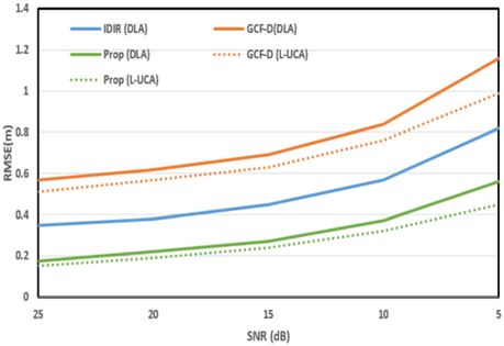
204   Page 10 of 12                                                                 Sådhanå (2020)45:204

Table 4. RMSE (m) in localization shown distinctly for two     percentage of computation required with an increase in the
sources (Src1, Src2) on SMARD database.                        number of delay segments. As shown, the percentage of
                                                               necessary calculations initially reduces exponentially and
                Anechoic signals        Reverberant signals    afterwards follows the constant trajectory.
Technique      Src 1       Src 2        Src 1        Src 2
IDIR            0.18        0.41        0.34          0.86     4.2 Performance evaluation with SMARD
GCF-D           0.23        0.63        0.59          1.08
Prop            0.11        0.13        0.19          0.25
                                                               database
                                                               SMARD database [40] has multichannel recordings of
                                                               anechoic and reverberant signals with different sensor
                                                               arrays configuration in a room with dimension 7:34 m
                                                               8:09 m  2:87 m at Aalborg University. The proposed
                                                               method is tested on the recording of anechoic and rever-
                                                               berant signals on configuration 0011 and 0111 having
                                                               sensors array placement identical to that of figure 8c. These
                                                               configurations have the sources placed at (2.00, 6.50, 1.25)
                                                               and at (3.50, 4.50, 1.50) with angle - 90 and - 45
                                                               respectively in XY-plane. The received signals at the
                                                               respective sensors in these configurations are added to get
                                                               the resultant of the two sources (cf. Eq. 1). The perfor-
                                                               mance evaluation of the proposed and existing method for
                                                               source localization is tabulated in Table 4 for anechoic and
                                                               reverberant signals differently. From these results, it is
                                                               observed that the proposed method outdoes the state-of-art
                                                               methods.
Figure 12. Physical set-up for AV16.3 and speakers locations
for seq37-3p-0001.
                                                               4.3 Evaluation using audio visual 16.3 (AV16.3)
                                                               corpus
ten delay segmentation for each pair, which is immensely
lesser than the other two.                                     In this section, experimental evaluation of the proposed
   A further study is carried out to observe the impact of     method is done using sequences seq01-1p-0000 and seq37-
delay segmentation on the computation cost in the spatial      3p-0001 for one and three speakers, respectively, selected
mapping of the estimated TDOAs. Figure 11 presents the         from Audio Visual 16.3 corpus (AV 16.3) [41]. The corpus

Figure 13. Ground truth of DOAs’of the sequences. (a) seq01-1p-0000 (1 speaker), (b) seq37-3p-0001 (3 speakers) from AV16.3
corpus.
Sådhanå (2020)45:204 Page 11 of 12 204
Table 5. The RMSE (m) in localization of the speaker(s) in the References
sequences seq01-1p-0000 and seq37-3p-0001 of AV 16.3
database. [1] Cobos M, Antonacci F, Alexandridis A, Mouchtaris A and
Lee B 2017 A survey of sound source localization methods
seq37-3p-0001 in wireless acoustic sensor networks. Wirel. Commun. Mob.
seq01-1p-0000
Technique Sp1 Sp1 Sp2 Sp3 Comput. 2017: 1–24. https://doi.org/10.1155/2017/3956282
[2] Li P and Ma X 2009 Robust acoustic source localization with
IDIR 0.58 0.81 0.24 0.41 TDOA based RANSAC algorithm. In: Proceedings of
GCF-D 0.67 1.01 0.27 0.51 Emergency Intelligent Computing Technology and Applica-
Prop 0.21 0.31 0.12 0.15 tions ICIC 2009. Lecture Notes Computer Science, vol. 5754.
Springer, Berlin, Heidelberg, pp. 222–227
was recorded in IDIAP meeting room of size 8:2 m [3] Argentieri S, Danès P and Souères P 2014 A survey on sound
3:6 m 2:4 m using the two circular microphone arrays source localization in robotics: from binaural to array
processing methods. \ hal-01058575 [ 1–32. https://doi.
(MA1 & MA2) where the possible speaker location is
org/10.1016/j.csl.2015.03.003
limited to an L shape area of 2 m 3 m, as shown in fig-
[4] Shen H, Ding Z, Dasgupta S and Zhao C 2014 Multiple
ure 12. The ground truth of direction of arrival (DOA) of a source localization in wireless sensor networks based on time
single active speaker in the sequences seq01-1p-0000 of arrival measurement. IEEE Trans. Signal Process. 62:
(217 sec) and three speakers in the seq37-3p-0001 1938–1949. https://doi.org/10.1109/TSP.2014.2304433
(511 sec) in different frames (frame length = 1 sec, sam- [5] Benesty J 2000 Adaptive eigenvalue decomposition algo-
pling frequency = 16 KHz) are shown in figure 13a and b rithm for passive acoustic source localization. J. Acoust. Soc.
respectively. These DOAs were converted to spatial coor- Am. 107: 384–391. https://doi.org/10.1121/1.428310
dinates to find the localization error of the corresponding [6] Knapp C H and Carter G C 1976 The generalized correlation
location estimates. For enhanced spatial sensitivity, the method for estimation of time delay. IEEE Trans. Acoust. 24:
proposed method and GCF-D are implemented, selecting 320–327. https://doi.org/10.1109/tassp.1976.1162830
[7] Alameda-Pineda X and Horaud R 2012 Geometrically-
four alternating microphones from each array, i.e., MA1
constrained robust time delay estimation using non-coplanar
and MA2, whereas IDIR is implemented with MA1 for
microphone arrays. In: Proceedings of 20th EUSIPCO,
competitive comparison. The spatial localization error Bucharest, Romania, pp. 1309–1313
(RMSE) of each source is tabulated in separate columns in [8] Hosseini M S, Rezaie A H and Zanjireh Y 2017 Time
Table 5 for both the sequences. As indicated by results, the difference of arrival estimation of sound source using cross
localization error of the speakers is in the order correlation and modified maximum likelihood weighting
Sp2\Sp3\Sp1 for the sequence seq37-3p-0001. Further, function. Sci. Iran 24: 3268–3279. https://doi.org/10.24200/
the proposed method has performed superior to the other sci.2017.4355
two existing methods for both the sequences. [9] Benesty J, Chen J and Huang Y 2004 Time-delay estimation
via linear interpolation and cross correlation. IEEE Trans.
Speech Audio Process. 12: 509–519. https://doi.org/10.1109/
TSA.2004.833008
5. Conclusions
[10] Liu H, Yang B and Pang C 2017 Multiple sound source
localization based on TDOA clustering and multi-path
This paper intends to provide a proficient TDOA based matching pursuit. In: Proceedings of IEEE ICASSP, New
method for localizing multiple sources. The method Orleans, LA, pp. 3241–3245
resolves the TDOA association ambiguities of the multiple [11] Dmochowski J P, Benesty J and Affes S 2007 A generalized
sources using volumetric mapping and eliminates the need steered response power method for computationally viable
to solve the complex hyperbolic equations for position source localization. IEEE Trans. Audio, Speech Lang.
estimation. The calculation of TDOA bounds of each sub- Process. 15: 2510–2526. https://doi.org/10.1109/TASL.
volume, delay segmentation and subvolume clustering is 2007.906694
done initially only and hence cut-off the required run-time [12] Sundar H, Sreenivas T V and Seelamantula C S 2018 TDOA-
based multiple acoustic source localization without associ-
computations. Moreover, the latter two steps together
ation ambiguity. IEEE/ACM Trans. Audio, Speech, Lang.
diminish the necessary subvolume scanning for delay
Process. 26: 1976–1990. https://doi.org/10.1109/TASLP.
mapping significantly and make the method computation- 2018.2851147
ally more efficient. The localization of the multiple sources [13] Smith J O and Abel J S 1987 Closed-form least-squares
is dramatically improved in adverse acoustic conditions by source location estimation from range-difference measure-
assigning equal weights to the mapped subvolumes for all ments. IEEE Trans. Acoust. 35: 1661–1669. https://doi.org/
the estimated delays. Moreover, the method shows 10.1109/TASSP.1987.1165089
enhanced localization results over the state-of-the-art [14] Alameda-Pineda X and Horaud R 2014 A geometric
techniques in adverse acoustic conditions. Finally, any approach to sound source localization from time-delay
desired resolution can be achieved by implementing C-SRP estimates. IEEE Trans. Audio, Speech Lang. Process. 22:
in the selected subvolume. 1082–1095. https://doi.org/10.1109/TASLP.2014.2317989204 Page 12 of 12 Sådhanå (2020)45:204
[15] Bestagini P, Compagnoni M, Antonacci F, Sarti A and [28] Hadad E and Gannot S 2018 Multi-Speaker Direction of
Tubaro S 2014 TDOA-based acoustic source localization in Arrival Estimation using SRP-PHAT Algorithm with a
the space–range reference frame. Multidim. Syst. Signal Weighted Histogram. In: Proceedings of International
Process. 25: 337–359. https://doi.org/10.1007/s11045-013- Conference on the Science of Electrical Engineering, Israel,
0233-8 pp. 1–5
[16] Jin B, Xu X and Zhang T 2018 Robust time-difference-of- [29] Brutti A, Omologo M, Member E and Svaizer P 2010
arrival (TDOA) localization using weighted least squares Multiple source localization based on acoustic map de-
with cone tangent plane constraint. Sensors 18: 1–16. https:// emphasis. EURASIP J. Audio, Speech, Music Process 2010:
doi.org/10.3390/s18030778 1–17. https://doi.org/10.1155/2010/147495
[17] Kwon B, Park Y and Park Y S 2010 Analysis of the GCC- [30] Lima M V S, Martins W A, Nunes L O, Biscainho L W P,
PHAT technique for multiple sources. In: Proceedings of Ferreira T N, Costa M V M and Lee B 2015 A volumetric
International Conference on Control, Automation and Sys- SRP with refinement step for sound source localization.
tems (ICCAS), Gyeonggi-do, pp. 2070–2073 IEEE Signal Process. Lett. 22: 1098–1102. https://doi.org/
[18] Claudio E D Di, Parisi R and Orlandi G 2000 Multi-source 10.1109/LSP.2014.2385864
localization in reverberant environments by root-music and [31] Cobos M, Marti A and Lopez J J 2010 A Modified SRP-
clustering. In: Proceedings of IEEE ICASSP, Istanbul, PHAT Functional for Robust Real-Time Sound Source
Turkey, pp. 921–924 Localization With Scalable Spatial Sampling. IEEE Signal
[19] Lathoud G and Odobez J 2007 Short-term spatio–temporal Process. Lett. 18: 71–74. https://doi.org/10.1109/lsp.2010.
clustering applied to multiple moving speakers. IEEE Trans. 2091502
Audio Speech Lang. Process. 15: 1696–1710 [32] Cobos M 2014 A note on the modified and mean-based
[20] Hu J S, Yang C H and Wang C K 2009 Estimation of sound steered-response power functionals for source localization in
source number and directions under a multi-source environ- noisy and reverberant environments. In: Proceedings of
ment. In: Proceedings of IEEE/RSJ International Conference IEEE 6th International Symposium on Communication,
on Intelligent Robot System 1: 181–186. https://doi.org/10. Control and Signal Process, Athens, pp. 149–152
1109/IROS.2009.5354706 [33] Lehmann E A and Johansson A M 2010 Diffuse reverberation
[21] Lee B and Choi J S 2010 Multi-source sound localization model for efficient image-source simulation of room impulse
using the competitive K-means clustering. In: Proceedings of responses. IEEE Trans. Audio, Speech Lang. Process. 18:
15th IEEE Conference on Emerging Technologies and 1429–1439. https://doi.org/10.1109/TASL.2009.2035038
Factory Automation, Bilbao, pp 1–7 [34] Lehmann E A and Johansson A M 2015 Prediction of energy
[22] Scheuing J and Yang B 2007 Efficient synthesis of decay in room impulse responses simulated with an image-
approximately consistent graphs for acoustic multi-source source model. J. Acoust. Soc. Am. 124: 269–277. https://doi.
localization. In: Proceedings of IEEE ICASSP, Honolulu, HI, org/10.1121/1.2936367
pp 501–504 [35] Kabal P 2002 TSP speech database. McGill Univ, Database
[23] Zannini C M, Cirillo A, Parisi R and Uncini A 2010 Version, pp. 1–39
Improved TDOA disambiguation techniques for sound [36] Fritts L 1997 University of Iowa musical instrument
source localization in reverberant environments. In: Pro- samples. In: Univ. Iowa. http://theremin.music.uiowa.edu/
ceedings of IEEE International Symposium on Circuits and MIS.html
Systems: Nano-Bio Circuit Fabrics and Systems, Paris, [37] Salvati D, Drioli C and Foresti G L 2017 Exploiting a
pp. 2666–2669 geometrically sampled grid in the steered response power
[24] Yang B and Kreißig M 2013 A graph-based approach to algorithm for localization improvement. J. Acoust. Soc. Am.
assist TDOA based localization. In: Proceedings of 8th 141: 586–601. https://doi.org/10.1121/1.4974289
International Workshop on Multidimensional System [38] Habets Emanuel and Sommen P C W 2002 Optimal
(nDS’13), Erlangen, Germany, pp. 75–80 microphone placement for source localization using time
[25] Levy A, Gannot S and Habets E A P 2011 Multiple- delay estimation. In: Proceedings of Workshop Circuits
hypothesis extended particle filter for acoustic source Systems and Signal Process. ProRISC, pp. 284–287
localization in reverberant environments. IEEE Trans. Audio [39] Brutti A, Omologo M and Svaizer P 2008 Localization of
Speech Lang. Process. 19: 1540–1555. https://doi.org/10. multiple speakers based on a two step acoustic map analysis.
1109/TASL.2010.2093517 In: Proceedings of IEEE ICASSP, Las Vegas, pp. 4349–4352
[26] Zotkin D N and Duraiswami R 2004 Accelerated speech [40] Nielsen J K, Jensen J R, Jensen S H and Christensen MG
source localization via a hierarchical search of steered 2014 The single-and multichannel audio recordings database
response power. IEEE Trans. Speech Audio Process. 12: (SMARD). In: Proceedings of 14th International Workshop
499–508. https://doi.org/10.1109/TSA2004.832990 Acoustic Signal Enhancement (IWAENC), pp. 40–44. https://
[27] Çöteli M B, Olgun O and Hacihabiboǧlu H 2018 Multiple doi.org/10.1109/IWAENC.2014.6953334
sound source localization with steered response power [41] Lathoud G, Odobez J and Gatica-Perez D 2004 AV16.3: An
density and hierarchical grid refinement. IEEE/ACM Trans. audio- visual corpus for speaker localization and tracking. In:
Audio Speech Lang. Process. 26:2215–2229. https://doi.org/ Proceedings of MLMI. Lecture Notes Computer Science, vol.
10.1109/TASLP.2018.2858932 3361. Springer, Berlin, Germany, pp. 182–195You can also read