Deep Active Learning for Joint Classification & Segmentation with Weak Annotator - export.arXiv.org
←
→
Page content transcription
If your browser does not render page correctly, please read the page content below

January 9, 2022                                                   Belharbi et al. [Accepted in WACV 2021]

                                         Deep Active Learning for Joint Classification &
                                         Segmentation with Weak Annotator

                                             Soufiane Belharbi1 , Ismail Ben Ayed1 , Luke McCaffrey2 , Eric Granger1
                                             1
                                               LIVIA, Dept. of Systems Engineering, École de technologie supérieure, Montreal, Canada
                                             2
                                               Goodman Cancer Research Centre, Dept. of Oncology, McGill University, Montreal, Canada
                                             soufiane.belharbi.1@ens.etsmtl.ca, {ismail.benayed, eric.granger}@etsmtl.ca, luke.mccaffrey@mcgill.ca
arXiv:2010.04889v2 [cs.CV] 14 Nov 2020

                                                                                        A BSTRACT

                                                    CNN visualization and interpretation methods, like class-activation maps (CAMs),
                                                    are typically used to highlight the image regions linked to class predictions.
                                                    These models allow to simultaneously classify images and extract class-dependent
                                                    saliency maps, without the need for costly pixel-level annotations. However, they
                                                    typically yield segmentations with high false-positive rates and, therefore, coarse
                                                    visualisations, more so when processing challenging images, as encountered in
                                                    histology. To mitigate this issue, we propose an active learning (AL) framework,
                                                    which progressively integrates pixel-level annotations during training. Given train-
                                                    ing data with global image-level labels, our deep weakly-supervised learning model
                                                    jointly performs supervised image-level classification and active learning for seg-
                                                    mentation, integrating pixel annotations by an oracle. Unlike standard AL methods
                                                    that focus on sample selection, we also leverage large numbers of unlabeled images
                                                    via pseudo-segmentations (i.e., self-learning at the pixel level), and integrate them
                                                    with the oracle-annotated samples during training. We report extensive experiments
                                                    over two challenging benchmarks – high-resolution medical images (histology
                                                    GlaS data for colon cancer) and natural images (CUB-200-2011 for bird species).
                                                    Our results indicate that, by simply using random sample selection, the proposed
                                                    approach can significantly outperform state-of the-art CAMs and AL methods,
                                                    with an identical oracle-supervision budget. Our code is publicly available.

                                         1      Introduction

                                         Image classification and segmentation are fundamental tasks in many visual recognition applications
                                         involving natural and medical images. Given a large image dataset annotated with global image-
                                         level labels for classification or with pixel-level labels for segmentation, deep learning (DL) models
                                         achieve state-of-the-art performances for these tasks (Dolz et al., 2018; Goodfellow et al., 2016;
                                         Krizhevsky et al., 2012; Litjens et al., 2017; Long et al., 2015; Ronneberger et al., 2015). However, the
                                         impressive accuracy of such fully-supervised learning models comes at the expense of a considerable
                                         cost for collecting and annotating large image data sets. While the acquisition of global image-
                                         level annotation can be relatively inexpensive, pixel-wise annotation involves a laborious process,
                                         a difficulty further accrued by the requirement of domain expertise, as in medical imaging, which
                                         increases the annotation costs.
                                         Weakly-supervised learning (WSL) has recently emerged as a paradigm that relaxes the need for
                                         dense pixel-wise annotations (Rony et al., 2019; Zhou, 2017). WSL techniques depend on the type of
                                         application scenario and annotation, such as global image-level labels (Belharbi et al., 2019b; Kim
                                         et al., 2017; Pathak et al., 2015; Teh et al., 2016; Wei et al., 2017), scribbles (Lin et al., 2016; Tang
                                         et al., 2018), points (Bearman et al., 2016), bounding boxes (Dai et al., 2015; Khoreva et al., 2017) or
                                         global image statistics such as the target-region size (Bateson et al., 2019; Jia et al., 2017; Kervadec

                                            Code: https://github.com/sbelharbi/deep-active-learning-for-joint-classification-and-segmentation-with-
                                         weak-annotator

                                                                                               1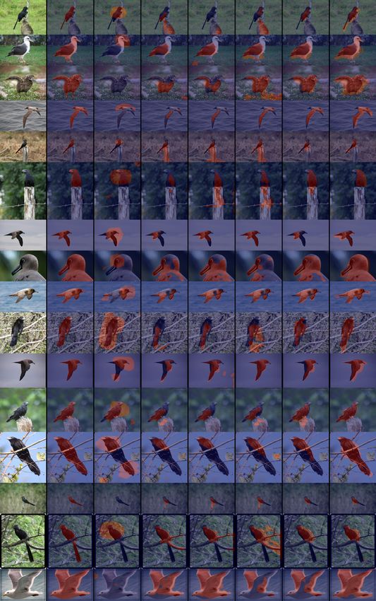
January 9, 2022                                                Belharbi et al. [Accepted in WACV 2021]

                      Figure 1: Proposed AL framework with weak annotator.

et al., 2019a;b). This paper focuses on learning using only image-level labels, which enables to
classify an image while yielding pixel-wise scores (i.e., segmentations), thereby localizing the regions
of interest linked to the image-class predictions.
Several CNN visualization and interpretation methods have recently been proposed, based on either
perturbation, propagation or activation approaches, and allowing to localize the salient image regions
responsible for a CNN’s predictions (Fu et al., 2020). In particular, WSL techniques (Rony et al.,
2019) rely on activation-based methods like CAM and, more recently, Gradient-weighted Class
Activation Mapping (Grad-CAM), Grad-CAM++, Ablation-CAM and Axiom-based Grad-CAM
(Fu et al., 2020; Lin et al., 2013; Pinheiro and Collobert, 2015). Trained with only global image-
level annotations, these methods locate the regions of interest (ROIs) of the corresponding class
in a relatively inexpensive and accurate way. However, while these WSL techniques can provide
satisfying results in natural images, they typically yield poor segmentations in relatively more
challenging scenarios, for instance, histology data in medical image analysis (Rony et al., 2019).
We note two limitations associated with CAMs: (1) they are obtained in an unsupervised way (i.e.
without pixel-level supervision under an ill-posed learning problem (Choe et al., 2020)); and (2) they
have low resolution. For instance, CAMs obtained from ResNet models (He et al., 2016) have a
resolution of 1/32 of the input image. Interpolation is required to restore full image resolution. Both
of these limitation with CAM-based methods lead to high false-positive rates, which may render
them impractical (Rony et al., 2019).
Enhancing deep WSL models with pixel-wise annotation, as supported by a recent study in weakly-
supervised object localization (Choe et al., 2020), can improve localization and segmentation accuracy,
which is the central goal of this paper. To do so, we introduce a deep WSL model that allows
supervised learning for classification, and active learning for segmentation, with the latter providing
more accurate and high-resolution masks. We assume that the images in the training set are globally
annotated with image-class labels. Relevant images are gradually labeled at the pixel level through
an oracle that respects a low annotation-budget constraint. Consequently, this leads us to an active
learning (AL) paradigm (Settles, 2009), where an oracle is requested to annotate pixels in a subset of
samples.
Different sample-acquisition techniques have been successfully applied to deep AL for classification
based on, e.g., certainty (Ducoffe and Precioso, 2015; Gal et al., 2017; Kirsch et al., 2019) or
representativeness (Kim et al., 2020; Sinha et al., 2019). However, very few deep AL techniques
were investigated in the context of segmentation (Gaur et al., 2016; Górriz Blanch, 2017; Lubrano di
Scandalea et al., 2019). Most AL techniques focus mainly on the sampling criterion (Fig.1, left) to
populate the labeled pool using an oracle. During training, only the labeled pool is used, while the
unlabeled pool is left dormant. Such an AL protocol may limit the accuracy of DL models under
constrained oracle-supervision budget in real-world applications for multiple reasons:
(1) Standard AL protocols may be relevant to small/shallow models that can learn and provide reliable
queries using a few training samples. Since training accurate DL models typically depends on large
training sets, large numbers of queries may be needed to build reliable DL models, which may incur
a high annotation cost.

                                                   2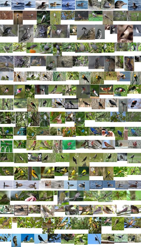
January 9, 2022                                                       Belharbi et al. [Accepted in WACV 2021]

(2) In most AL work, the experimental protocol starts with a large labeled pool, and acquires a large
number of queries for sufficient supervision, neglecting the workload placed on the oracle. This
typically reaches a plateau-performance of a DL quickly, hampering a reliable study of the impact
of different AL selection techniques. Moreover, model-based sampling techniques are inconsistent
(Gaur et al., 2016) in the sense that the model is used to query samples while it is still in an early
learning stage.
(3) Segmentation and classification problems are associated with different properties and challenges,
such as decision boundaries and uncertainty, which provide additional challenges to AL. For instance,
the class boundaries defined by different classification methods (Ducoffe and Precioso, 2018; Settles,
2009; Tong and Koller, 2001) are not defined in the context of segmentation, making such a branch
of methods inadequate for segmentation.
(4) In critical fields such as medical imaging, acquiring a sample itself can be very expensive1 . The
time and cost associated with each sample makes them valuable items. Such considerations may be
overlooked for large-scale data sets with almost-free samples, as in the case of natural images. Given
this high cost, keeping the unlabeled pool dormant during learning may be ineffective.
Based on the aforementioned arguments, we advocate that focusing solely on the sample acquisition
and supervision pool may not be an efficient way to build high-performing DL models in an AL
framework for segmentation. Therefore, we consider augmenting the labeled pool using the model as
a second source of annotation, in a self-learning fashion (Mao, 2020) (Fig.1, right). This additional
annotation might be less accurate (i.e., weak2 ) compared to the oracle that provides strong but
expensive annotations. However, it is expected to fast-improve the model’s performance (Mao, 2020),
while using a few oracle-annotated samples, reducing the annotation cost.
Our main contributions are the following. (1) Architecture design: As an alternative to CAMs,
we propose using a segmentation mask trained with pixel-level annotations, which yields more
accurate and high-resolution ROIs. This is achieved through a convolutional architecture capable
of simultaneously classifying and segmenting images, with the segmentation task trained using
annotations acquired using an AL framework. As illustrated in Fig.3, the architecture combines well-
known DL models for classification (ResNet (He et al., 2016)) and segmentation (U-Net (Ronneberger
et al., 2015)), although other architectures could also be used. (2) Active learning: We augment
the size of the labeled pool by weak-annotating a large number of unlabeled samples based on
predictions of the DL model itself, providing a second source of annotation (Fig.1). This enables
rapid improvements of the segmentation accuracy, with less oracle-based annotation. Moreover, our
method can be integrated on top of any sample-acquisition method. (3) Experimental study: We
conducted comprehensive experiments over two challenging benchmarks – high-resolution medical
images (histology GlaS data for colon cancer) and natural images (CUB-200-2011 for bird species).
Our results indicate that, by simply using random sample selection, the proposed approach can
significantly outperform state-of the-art CAMs and AL methods, with an identical oracle-supervision
budget.

   1
      For instance, prior to a diagnosis of breast cancer from a histological sample, a patient undergoes a bilateral
diagnostic mammogram and breast ultrasound that are interpreted by a radiologist, one to several needle biopsies
(with low risks under 1% of hematoma and wound infection) to further assess areas of concern, surgical
consultation and pre-operative blood work, and surgical excision of the positive tissue for breast cancer cells.
The biopsy and surgical tissues are processed (fixation, embedding in parraffin, H&E staining) and interpreted
by a pathologist. Depending on the cancer stage, the patient may undergo additional procedures. Therefore,
accounting for all the steps required for breast cancer diagnosis from histological samples, a rough estimation of
the final cost associated with obtaining a Whole Slide Image (WSI) is about $400 (Canadian dollars, by 1999)
(Will et al., 1999). Moreover, some cancer types are rare (Will et al., 1999), adding to the values of these samples.
All these procedures are conducted by highly trained experts, with each procedure taking from a few minutes to
an hour and requiring expensive specialized medical equipment.
    2
      Not to be confused with the weak annotation of data in weakly supervised learning frameworks.

                                                         3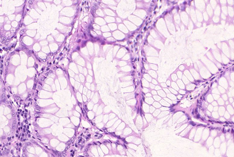
January 9, 2022                                                 Belharbi et al. [Accepted in WACV 2021]

2   Related work

Deep active learning: AL has been studied for a long time in machine learning, mainly for classifi-
cation and regression, using linear models in particular (Settles, 2009). Recently, there has been an
effort to transfer such techniques to DL models for classification tasks by mimicking their intuition or
by adapting them, taking into consideration model specificity and complexity. Such methods include,
for instance, different mechanisms for uncertainty (Beluch et al., 2018; Ducoffe and Precioso, 2015;
2018; Gal et al., 2017; Kim et al., 2020; Kirsch et al., 2019; Lakshminarayanan et al., 2017; Wang
et al., 2016; Yoo and Kweon, 2019) and representativeness estimation (Kim et al., 2020; Sener and
Savarese, 2018; Sinha et al., 2019). However, most deep AL techniques are validated on synthetic,
simple or tiny data, which does not explore their full potential in real applications.
While deep AL for classification is rapidly growing, deep AL models for segmentation are uncommon
in the literature. In fact, the very few methods in the literature mostly focused on the direct application
of deep AL classification methods. The limited research in this area may be explained by the fact
that segmentation tasks bring challenges to AL, such as the additional spatial information and the
fact that a segmentation mask lies in a much larger dimension than a classification prediction. In
classification, AL often deals with one output that is used to drive queries (Huang et al., 2010). The
spatial information in segmentation does not naturally provide a direct scoring function that can
indicate the overall quality or certainty of the output. Most of deep AL methods for segmentation
consider pixels as classification instances, and apply standard AL techniques to each pixel.
For instance, the authors of (Gaur et al., 2016) exploit a variant of entropy-based acquisition at
the pixel level, combined with a distribution-based term that encodes diversity using a complex
hierarchical clustering algorithm over sliding windows, with application to microscopic membrane
segmentation. Similarly, (Górriz Blanch, 2017; Lubrano di Scandalea et al., 2019) apply Monte-Carlo
dropout uncertainty (Gal et al., 2017) at the pixel level, with application to myelin segmentation
using spinal cord and brain microscopic histology images. In (Roels and Saeys, 2019), the authors
experiment with five acquisition functions of classification for a segmentation task, including entropy-
based, core-set (Sener and Savarese, 2018), k-mean and Bayesian (Gal et al., 2017) sampling, with
application to electron microscopy segmentation. Entropy-based methods seem to be dominant over
multiple datasets. In (Yang et al., 2017), the authors combine two sampling terms for histology image
segmentation. The first employs bootstrapping over fully convolutional networks (FCN) to estimate
uncertainty, where a set of FCNs are trained on different subsets of samples. The second term is a
representation-based term that selects the most representative samples. This is achieved by solving
an optimization of a generalization version of the maximum cover set problem (Feige, 1998) using
sample description extracted from an FCN. Despite the obtained promising results, this approach
remains complex and impractical due to the use of bootstrapping over DL models and an optimization
step. Moreover, the authors of (Yang et al., 2017) do not provide a comparison to other acquisition
functions. The work in (Casanova et al., 2020) considers a specific case of AL using reinforcement
learning for region-based AL for segmentation, where only a selected region of the image is labeled.
This method is adequate for data sets with large and unbalanced classes, such as street-view images.
While the method in (Casanova et al., 2020) outperforms random and Bayesian (Gal et al., 2017)
selection, surprisingly, it performs close to entropy-based selection.
Weak annotators: The AL paradigm does not prohibit the use of unlabelled data for training (Settles,
2009), but it mainly constrains the oracle-labeling budget. The standard AL experimental protocol
(Fig.1, left) was inherited from AL of simple/linear ML models, and adopted in subsequent works.
Budget-constrained oracle annotation may not be sufficient to build effective DL models, due to
the lack of labeled samples. Furthermore, several studies in AL for classification have successfully
leveraged the unlabelled data to provide additional supervision (Lin et al., 2017; Long et al., 2008;
Vijayanarasimhan and Grauman, 2012; Wang et al., 2016; Zhou et al., 2010; Zhu et al., 2003).
For instance, the authors of (Lin et al., 2017; Wang et al., 2016) propose to pseudo-label a part of the
unlabeled pool. The latter is selected using dynamic thresholding based on confidence, through the
model itself, so as to learn a better embedding. Furthermore, a theoretical framework for AL using
strong and weak annotators for classification task is introduced in (Zhang and Chaudhuri, 2015). Their
results suggest that using multiple annotators can reduce the cost of oracle annotation, in comparison

                                                    4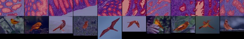
January 9, 2022                                               Belharbi et al. [Accepted in WACV 2021]

to one annotator. Multiple sources of annotations that include both strong and weak annotators
were used in AL, crowd-sourcing, self-paced learning and other interactive learning scenarios for
classification to help reducing the number of requests for the strong annotator (Kremer et al., 2018;
Malago et al., 2014; Mattsson, 2017; Murugesan and Carbonell, 2017; Urner et al., 2012; Yan et al.,
2016; Zhang and Chaudhuri, 2015). Using the model itself for pseudo-annotation is motivated mainly
by the success of deep self-supervised learning (Mao, 2020).
Label Propagation (LP): Our approach is also related to
LP methods (Bengio et al., 2010; Zhou et al., 2004; Zhu
and Ghahramani, 2002) for classification, which aim to
label unlabeled samples using knowledge from the labeled
ones (Fig.2). However, while LP propagates labels to un-
labeled samples through an iterative process, our approach
bypasses this using the model itself. In our case, the
propagation is limited to the neighbors of labeled samples
defined through k-nearest neighbors (k-nn) (Fig.2). Using
k-nn has been also studied to combine AL and domain
adaptation (Berlind and Urner, 2015), where the goal is to
query samples from the target domain. Such an approach
is connected to the recently developed core-set method for
deep AL (Sener and Savarese, 2018). Our method inter-
sects with (Berlind and Urner, 2015) only in the sense of
predicting the labels to query samples using their labeled Figure 2: The k-nn method for select-
neighbors.                                                    ing U00 subset to be speudo-labeled. As-
                                                              sumption to select U00 : since U00 lives
In contrast to state-of-the-art DL models for AL segmen- nearby supervised samples, it is more
tation, we consider increasing the unlabeled pool through likely to be assigned good segmentation
pseudo-annotated samples (Fig.1, right). To this end, the by the model. We consider measuring
model is used for pseudo-labeling samples within the k-nn for each unlabeled sample. In this
neighborhood of samples with strong supervision (Fig.2). example, using k = 4 allows |U00 | = 14.
From a self-learning perspective, the works in (Lin et al., If k-nn is considered for each labeled
2017; Wang et al., 2016) on face recognition are the closest sample: |U00 | = 8. |·| is the set cardi-
to ours. While both rely on pseudo-labeling, they mainly nal. Note that k-nn is only considered
differ in the sample selection for pseudo-annotation. In between samples of the same class.
(Lin et al., 2017; Wang et al., 2016), the authors considered
model confidence, where samples with high confidence
are pseudo-labeled, while low-confidence samples are queried. While this yields good results, it
makes the overall method strongly dependent on model confidence. As we consider segmentation
tasks, model-confidence is not well-defined. Moreover, using the expected pixel-wise values can be
less representative for model confidence.
Our approach relies on the spatial assumption in Fig.2, where the samples to pseudo-label are selected
to be near the labeled samples, and expected to have good pseudo-segmentations. This makes the
oracle-querying technique independent from the pseudo-labeling method, giving more flexibility to
the user. Our pseudo-labeled samples are added to the labeled pool, along with the samples annotated
by the oracle. The underlying assumption is that, given a sample labeled by an oracle, the model is
more likely to produce good segmentations of images located nearby that sample. Our assumption is
verified empirically in the experimental section of this paper. This simple procedure enables to rapidly
increase the number of pseudo-labeled samples, and helps improving segmentation performance
under a limited amount of oracle-based supervision.

3   Proposed approach

We consider an AL framework for training deep WSL models, where all the training images have
class-level annotations, but no pixel-level annotations. Due to their high cost, pixel annotations are
gradually acquired for training through oracle queries. It propagate pixel-wise knowledge encoded in
the model though the labeled images.

                                                   5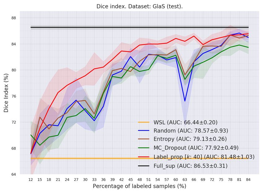
January 9, 2022                                                    Belharbi et al. [Accepted in WACV 2021]

Active learning training consists of sequential training
rounds. At each round r, the total training set D that con-
tains n samples with unlabeled and labeled subsets (Fig.1).
(1) Unlabeled subset: contains samples without pixel-
wise annotation (unlabeled samples) U = {xi , yi , −}ui=1
where x ∈ X is the input image, y is its global label;
and the pixel label is missing. (2) Labeled subset: con-
tains samples with full supervision L = {xi , yi , mi }li=1
where m is the pixel-wise annotation of the sample. L
is initially empty. It is gradually populated from U by
querying the oracle using an acquisition function. Let
f (· : θ) denotes a DL model that is able to classify and
segment an image x (Fig.3). For clarity, and since we
focus on the segmentation task, we omit the notation
for the classification task (to simplify the presentation).
Therefore, f (x) refers to the predicted segmentation mask.
Let U0 ⊆ U and U00 ⊆ U denote two subsets (Fig.1), with
U0 ∩ U00 = ∅. In our method, we introduce P as a sub-       Figure 3: Our proposed DL architecture
set holder for pseudo-labeled samples, which is initially   for classification and segmentation com-
empty and gradually replenished (Fig.1, right). To express  posed of: (1) a shared backbone for fea-
the dependency of each subset on round r, we introduce      ture extraction; (2) a classification head
the following notations: Ur , Lr , Pr , U0r , U00r . The samples
                                                            for the classification task; (3) and a seg-
in Pr are denoted as {xi , yi , m̂i }. The following holds: mentation head for the segmentation
∀r : D = Lr ∪ Ur ∪ Pr .                                     task with a U-Net style (Ronneberger
Alg.1 describes the overall AL process with our pseudo- et al., 2015). The latter merges rep-
annotation method. First, U0r is queried, then labeled by resentations from the backbone, while
the oracle, and added to Lr . Using k-nn, U00r is selected gradually upscaling the feature maps to
based on their proximity to Lr (Fig.2); and pseudo-labeled reach the full image resolution for the
by the model, then added to Pr . To fast-increase the size predicted mask, similarly to the U-Net
of Lr , Pr is protected from being queried for the oracle model.
until it is inevitable. In the latter case, queried samples
from Pr are used to fill U0 ; and they are no longer considered pseudo-labeled since they will be
assigned the oracle annotation.
To measure image similarity for the k-nn method, we used the color distribution to describe image
content. This can be a flexible descriptor for highly unstructured images such as histology images.
Note that the k-nn method is considered only for pairs of samples of the same class. The underlying
assumption is that samples of the same class, with similar color distributions, are likely to contain
relatively similar objects. Consequently, labeling representative samples could be a proxy for
supervised learning based on the underlying data distribution. This can increase the likelihood of the
model to provide relatively good segmentations of the other samples. The proximity between two
images (xi , xj ) is measured using the Jensen-Shannon divergence between their respective color
distributions (measured as normalized histograms). For an image with multiple color planes, the
similarity is formulated as the sum of similarities, one for each plane.
At round r, the queried and pseudo-labeled samples are both used in training by optimizing the
following loss function:
                            X                        X
                      min        L(f (xi ), mi ) + λ      L(f (xi ), m̂i ),                (1)
                          θ
                              xi ∈Lr−1                      xi ∈Pr−1

where L(·, ·) is a segmentation loss, and λ a positive scalar. Eq.(1) corresponds to training the model
(Fig.3) solely for the segmentation task. Simultaneous training for classification and segmentation
in this AL setup is avoided due to the unbalance between the number of samples that are labeled
globally and at the pixel level. Therefore, we consider training the model for classification first. Then,
we freeze the classifier parameters. Training for the segmentation tasks is resumed later. This yields
the best classification performance, and allows a better study of the impact of the queried samples on
the segmentation task.

                                                      6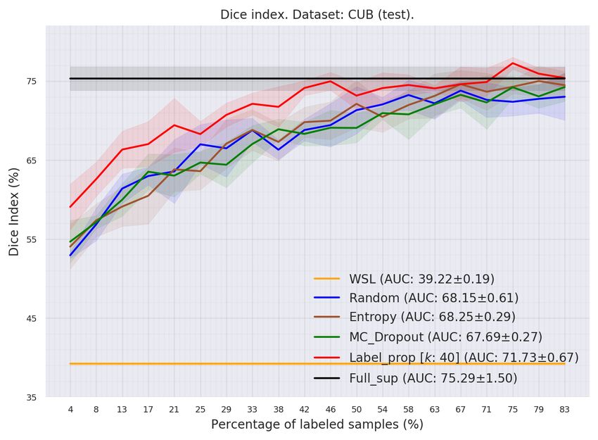
January 9, 2022                                                            Belharbi et al. [Accepted in WACV 2021]

Considering the relation of our method and label propagation algorithm (Bengio et al., 2010; Zhou
et al., 2004; Zhu and Ghahramani, 2002), we refer to our proposal as Label_prop.

                            Algorithm 1: Standard AL procedure and our proposal.
                            The extra instructions associated with our method are
                            indicated with a blue background .
                                 Input : P0 = L0 = ∅
                                         θ 0 : Initial parameters of f trained on the
                                 classification task.
                                         maxr : Maximum number of AL rounds.
                            1    Select U00 randomly and label them by an oracle.
                            2    L0 ← U00 .
                            3    for r ∈ 1 · · · maxr do
                            4        θ ← θ0 .
                            5        Train f using Lr−1 ∪ Pr−1 and the loss in Eq. (1).
                            6        Select U0r and label them by an oracle.
                            7        Lr ← Lr−1 ∪ U0r .
                            8         Select U00r .
                            9         Pr ← Pr−1 ∪ U00r .
                            10        Pseudo-label Pr .

4         Results and discussion

4.1        Experimental methodology:

a) Datasets. For evaluation, datasets should have global and pixel-wise annotation. We consider
two public datasets including both medical (histology) and natural images (Fig.4). (1) GlaS dataset:
This dataset contains histology images for colon cancer diagnosis3 (Sirinukunwattana et al., 2017). It
includes 165 images derived from 16 Hematoxylin and Eosin (H&E) histology sections of two grades
(classes): benign and malignant. It is divided into 84 samples for training and 80 samples for testing.
The ROIs to be segmented are the glandes. (2) CUB-200-2011 dataset (CUB)4 (Wah et al., 2011) is
a dataset for bird species with 11, 788 samples (5, 994 for training and 5, 794 for testing) and 200
species. The ROIs to be segmented are the birds. In GlaS and CUB datasets, we randomly select
80% of the training samples for effective training, and 20% for validation (with full supervision) to
perform early stopping. The splits are identical to the ones used in (Belharbi et al., 2019a; Rony et al.,
2019) (split 0, fold 0), and are publicly available.
b) Active learning setup. To assess the performance of different AL acquisition methods, we
consider a realistic scenario with respect to the number of samples to be labeled at each AL round,
      3
          GlaS: warwick.ac.uk/fac/sci/dcs/research/tia/glascontest.
      4
          CUB: www.vision.caltech.edu/visipedia/CUB-200-2011.html

Figure 4: Top row: GlaS dataset (Sirinukunwattana et al., 2017). Bottom row: CUB dataset (Wah
et al., 2011). (Best visualized in color.)

                                                              7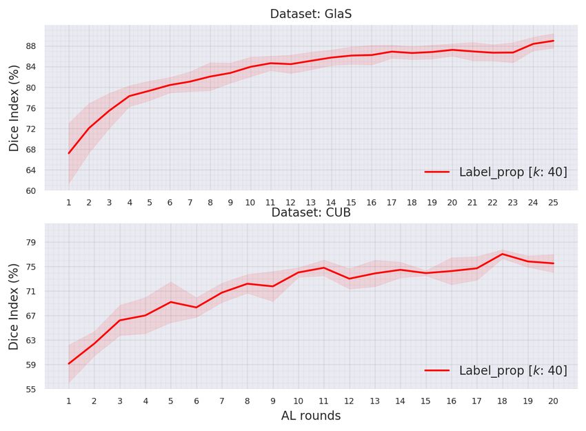
January 9, 2022                                                Belharbi et al. [Accepted in WACV 2021]

                   Table 1: Number of samples selected for the oracle per round.

                            #selected samples    #selected samples    Max AL rounds
                  Dataset
                            per-class (r = 1)    per-class (r > 1)    (maxr in Alg.1)
                  GlaS              4                    1                   25
                  CUB               1                    1                   20

accounting for the load imposed on the oracle. Therefore, only a few samples are selected at each
round for oracle annotation, and L is slowly replenished. This allows better comparison between AL
selection techniques since we spend more time in a phase where L holds a few samples. Such a phase
allows to better measure the impact of the selected samples. Filling L quickly brings the model’s
performance to a plateau that hides the impact of newly selected samples. The initial replenishment
(r = 1) is achieved by randomly selecting a few samples. The same samples are used for all AL
techniques at round r = 1 for a fair comparison. To avoid any bias from selecting unbalanced classes
that can directly affect the segmentation performance, and hinder AL evaluation, the same number
of samples is selected from each class (since the global annotation is known beforehand for all the
samples). Note that the oracle is used only to provide pixel-wise annotation. Tab.1 provides the
selection details.
c) Evaluation. We report the classification accuracy obtained by the classification head (Fig.3).
Average Dice index is used to measure the segmentation quality at each AL round forming a Dice
index curve over all the rounds. To better assess the dominance of each method (Settles, 2009), the
Area Under the Dice index Curve is used (AUC). This provides a fair indicator of the dominant curve,
but contrasts with standard AL works, where one or multiple specific operating points in the curve
are selected (leading to a biased and less accurate protocol). The average and standard deviation of
Dice index curve and AUC metric are reported based on 5 replications of a complete AL session,
using a different seed for each session. An AL session across different methods uses the same seed.
While our approach, referred to as (Label_prop), can operate on top of any AL selection criterion,
we demonstrate its efficiency using simple random selection, which is often a baseline for AL
experiments. Note that our pseudo-annotations are obtained from the segmentation head shown
in Fig.3. Our method is compared to three different AL selection approaches for segmentation:
(1) random selection (Random): the samples are randomly selected; (2) entropy-based selection
(Entropy): the scoring function per sample is the average entropy at the pixel level (Gaur et al., 2016).
Samples with high entropy are selected; and (3) Monte-Carlo dropout uncertainty (MC_Dropout):
we use Monte-Carlo dropout (Górriz Blanch, 2017; Lubrano di Scandalea et al., 2019) at the pixel
level to compute the uncertainty score per sample. Samples are forwarded 50 times in the model,
where dropout is set to 0.2 (Górriz Blanch, 2017; Lubrano di Scandalea et al., 2019). Then, the
pixel-wise variance is estimated. Samples with high mean variance are selected.
Lower bound performance (WSL): We consider the segmentation performance obtained by WSL
method as a lower bound. It is trained using only global annotation. CAMs are used to extract the
segmentation mask. WILDCAT method is considered (Durand et al., 2017) (Fig.3) at the classification
head to obtain the CAMs. For WSL method, a pre-trained model over ImageNet (Deng et al., 2009)
is used to initialize the weights of the backbone, which is then fined-tuned. The model is trained over
the entire dataset, where samples are labeled globally only. The obtained classifier using seed=0 is
frozen and used as a backbone for all the other methods.
Upper bound performance (Full_sup): Fully supervised segmentation is considered as an upper
bound on performance. The model in Fig.3 is trained for segmentation only using the entire dataset,
where samples are labeled at the pixel level.
For a fair comparison, all the methods are trained using the same hyper-parameters over the same
dataset. WSL and Full_sup methods have minor differences. Due to space limitation, all the hyper-
parameters are presented in the supplementary material. In Alg.1, notice that for our method, Pr is
not used at the current round r but until the next round r + 1. To take advantage of Pr at round r,
instructions from line-4 to line-10 are repeated twice in the provided results.

                                                   8
January 9, 2022 Belharbi et al. [Accepted in WACV 2021]
Table 2: Classification accuracy over of the proposed deep WSL model on GlaS and CUB test
datasets.
Dataset GlaS CUB
Classification
99.50 ± 0.61 73.22 ± 0.19
accuracy (%)
4.2 Results
(a) (b)
Figure 5: Average Dice index of the proposed and baseline methods over test sets. (a) GlaS. (b) CUB.
Table 3: Average AUC and standard deviation (Fig.5) for Dice index performance over GlaS and
CUB test sets.
Dataset GlaS CUB
WSL 66.44 ± 0.20 39.22 ± 0.19
Random 78.57 ± 0.93 68.15 ± 0.61
Entropy 79.13 ± 0.26 68.25 ± 0.29
MC_Dropout 77.92 ± 0.49 67.69 ± 0.27
Label_prop (ours) 81.48 ± 1.03 71.73 ± 0.67
Full_sup 86.53 ± 0.31 75.29 ± 1.50
We report the classification and segmentation performances following the training the proposed deep
WSL model in Fig.3. Tab.2 reports the Classification accuracy of the classification head using WSL,
which is close to the results reported in (Belharbi et al., 2019b; Rony et al., 2019). The results of
GlaS suggest that it is an easy dataset for classification.
The segmentation results are reported in Tabs. 4 and 3, and in Fig 5.
Fig. 5a compares Dice accuracy on the GlaS dataset. On the latter, we observe that adding more
labels increases Dice index for all AL methods, yielding, as expected, better performance than the
WSL method. Reading from Tab.4, randomly labeling only 4 samples per class enables to easily
outperform WSL. This means that using our approach in Fig.3, with limited supervision, can lead
to more accurate masks compared to using CAMs in the WSL method. From Fig.5a, one can
also observe that Random, Entropy, and MC_Dropout methods grow relatively in the same way,
leading to the same overall performance, with the Entropy method slightly ahead. Considering the
overall behavior of the curves, one may conclude that using advanced selection techniques such as
9January 9, 2022 Belharbi et al. [Accepted in WACV 2021]
Table 4: Readings of Dice index (mean ± standard deviation) from Fig.5 over test set for the first 5
queries formed by each method. We start from the second query since the first query is random but
identical for all methods.
Queries q2 q3 q4 q5 q6
GlaS
WSL 66.44 ± 0.20
Random 70.26 ± 3.02 71.58 ± 3.14 71.43 ± 1.83 74.05 ± 3.14 75.36 ± 3.45
Entropy 72.75 ± 2.96 70.93 ± 3.58 72.60 ± 1.44 73.44 ± 1.38 75.15 ± 1.63
MC_Dropout 68.44 ± 2.89 69.70 ± 1.96 69.97 ± 1.95 72.71 ± 2.21 73.00 ± 1.04
Label_prop (ours) 71.02 ± 4.19 74.07 ± 3.93 76.52 ± 3.49 77.63 ± 2.73 78.41 ± 1.23
Full_sup 86.53 ± 0.31
CUB
WSL 39.22 ± 0.18
Random 56.86 ± 2.07 61.39 ± 1.85 62.97 ± 1.13 63.56 ± 4.02 66.56 ± 2.50
Entropy 53.37 ± 2.06 59.11 ± 2.50 60.48 ± 3.56 63.81 ± 2.75 63.59 ± 2.34
MC_Dropout 57.13 ± 0.83 59.98 ± 2.06 63.52 ± 2.26 63.02 ± 2.68 64.68 ± 1.41
Label_prop (ours) 62.58 ± 2.15 66.32 ± 2.34 67.01 ± 2.85 69.40 ± 3.40 68.28 ± 1.60
Full_sup 75.29 ± 1.50
MC_Dropout and Entropy provides an accuracy similar to simple random selection. On the one hand,
since both methods have shown substantial improvements in AL for classification, and based on
the results in Fig.5a, one may conclude that all samples are equivalently informative for the model.
Therefore, there is no better order to acquire them. On the other hand, using simply random selection
and pseudo-labeled samples allowed our method to substantially improve the overall performance,
demonstrating the benefits of self-learning.
Fig.5b and Tab.4 compare Dice accuracy on the CUB dataset, where labeling only one sample per
class yielded a large improvement in Dice index, in comparison to WSL. Adding more samples
increases the performance of all the methods. One can observe similar pattern as for GlaS: Random,
Entropy and MC_Dropout methods yield similar curves, while the AUC performances of Random
and Entropy methods are similar, and slightly ahead of MC_Dropout. Similar to GlaS analysis, and
based on the results of these three methods, one can conclude that none of the methods for ordering
the samples is better than simple random selection. Using self-labeled samples in our method shows
again its benefits. Simple random selection combined with self-annotation yields an overall best
performance. Using two datasets, our empirical results suggest that self-learning, under limited
oracle-annotation, has the potential to provide a reliable second source of annotation, which can
efficiently enhance model performance, while using simple sample acquisition techniques.
Pseudo-annotation performance. Furthermore, the proposed approach is assessed on the pseudo-
labeled samples at each AL round. Fig.6 shows that the model provides good segmentations at
the initial rounds. Then, the more supervision, the more accurate the pseudo-segmentation, as
expected. This figure shows the interest and potential of self-learning in segmentation, and confirms
our assumption that samples near the labeled ones are likely to achieve accurate pseudo-segmentation
by the model.
Hyper-parameters. Our approach requires two main hyper-parameters: k and λ. We conducted an
ablation study over k on GlaS dataset, and over λ on both datasets. Results, which are presented
in the supplementary material, suggest that our method is less sensitive to k. λ plays an important
role, and based on our study, we recommend using small values of this weighting parameter. In
our experiments, we used λ = 0.1 for Glas and λ = 0.001 for CUB. We set k = 40. We note that
hyper-parameter tuning in AL is challenging due to the change of the size of the data set, which in
turn changes the training dynamics. In all the experiments, we used fixed hyper-parameters across the
AL rounds. Fig.6 suggests that a dynamic λ(r) that is increased through AL rounds could be more
10January 9, 2022 Belharbi et al. [Accepted in WACV 2021]
Figure 6: Average Dice index over the pseudo-labeled samples of our method in each AL round.
beneficial. However, this requires a principled update protocol for λ, which was not explored in this
work. Nonetheless, using a fixed value seems to yield promising results overall.
Supplementary material. Due to space limitation, we deferred the hyper-parameters used in the
experiments, results of the ablation study, visual results for the similarity measure and examples of
predicted masks to the supplementary materials.
5 Conclusion
Deep WSL models trained with global image-level annotations can play an important role in CNN
visualization and interpretability. However, they are prone to high false-positive rates, especially
for challenging images, leading to poor segmentations. To alleviate this issue, we considered using
pixel-wise supervision provided gradually through an AL framework. This annotation is integrated
into training using an adequate deep convolutional model that allows supervised learning for both
tasks: classification and segmentation. Through a few pixel-supervised samples, such a design is
intended to provide full-resolution and more accurate masks compared to standard CAMs, which
are trained without pixel supervision and often provide coarse resolution. Therefore, it enables a
better CNN visualization and interpretation of CNN predictions. Furthermore, and unlike standard
deep AL methods that focus solely on the acquisition function, we considered using self-learning
as a second source of supervision to fast-improve the model segmentation. Evaluating our method
using a realistic AL protocol over two challenging benchmarks, our results indicate that: (1) using a
few supervised samples, the proposed architecture yielded more accurate segmentations compared
to CAMs, with a large margin using different AL methods. Thus, it provides a solution to enhance
pixel-wise predictions in real-world visual recognition applications. (2) using self-learning with
random selection yielded substantial improvements. Self-learning under a limited oracle-budget can,
therefore, provide a cost-effective alternative to standard AL protocols, where most of the effort is
spent on the acquisition function.
Acknowledgment
This research was supported in part by the Canadian Institutes of Health Research, the Natural
Sciences and Engineering Research Council of Canada, Compute Canada, MITACS, and the Ericsson
Global AI Accelerator Montreal.
11January 9, 2022 Belharbi et al. [Accepted in WACV 2021]
A Supplementary material for the experiments
Due to space limitation, we provide in this supplementary material detailed hyper-parameters used in
the experiments, results of the ablation study, visual results to the similarity measure, and examples
of predicted masks.
A.1 Training hyper-parameters
Tab.5 shows the used hyper-parameters in all our experiments.
Table 5: Training hyper-parameters.
Hyper-parameter GlaS CUB
Model backbone ResNet-18 (He et al., 2016)
WILDCAT (Durand et al., 2017):
α 0.6
kmin 0.1
kmax 0.1
modalities 5
Optimizer SGD
Nesterov acceleration True
Momentum 0.9
Weight decay 0.0001
Learning rate (LR) 0.1 (WSL: 10−4 ) 0.1 (WSL: 10−2 )
LR decay 0.9 0.95 (WSL: 0.9)
LR frequency decay 100 epochs 10 epochs
Mini-batch size 20 8
Learning epochs 1000 30 (WSL: 90)
Horizontal random flip True
Vertical random flip True False
Crop size 416 × 416
k 40
λ 0.1 0.001
A.2 Ablation study
We study the impact of k and λ on our method. Results are presented in Fig.7, 8 for GlaS over
k, λ; and in Fig.9 for CUB over λ. Due to the expensive computation time required to perform AL
experiments, we limited the experiments (k, λ, number of trials, and maxr). The obtained results
of this study show that our method is less sensitive to k (standard deviation of 0.59 in Fig.7). In
other hand, the method shows sensitivity to λ as expected from penalty-based methods (Bertsekas,
1999). However, the method seems more sensitive to λ in the case of CUB than GlaS. CUb dataset
is more challenging leading to more potential erroneous pseudo-annotation. Using Large λ will
systematically push the model to learn on the wrong annotation (Fig.9) which leads to poor results.
In the other hand, GlaS seems to allow obtaining good segmentation where using large values of
λ did not hinder the performance quickly (8). The obtained results recommend using small values
that lead to better and stable performance. Using high values, combined with the pseudo-annotation
errors, push the network to learn erroneous annotation leading to overall poor performance.
12January 9, 2022 Belharbi et al. [Accepted in WACV 2021]
Figure 7: Ablation study over GlaS dataset (test set) over the hyper-parameter k (x-axis). y-axis: AUC
of Dice index (%) of 25 queries for one trial. AUC average ± standard deviation: 81.49 ± 0.59.
Best performance in red dot: k = 40, AU C = 82.41%.
Figure 8: Ablation study over GlaS dataset (test set) over the hyper-parameter λ (x-axis). y-axis:
AUC of Dice index (%) of 15 queries for one trial. Best performance in red dot: λ = 0.1, AU C =
79.15%.
A.3 Similarity measure
In this section, we present some samples with their nearest neighbors. Although, it is difficult to
quantitatively evaluate the quality of such measure. Fig.10 shows the case of GlaS. Overall, the
similarity shows good behavior of capturing the general stain of the image which is what was intended
for since the structure of such histology images is subject to high variation. Since the stain variation
is one of the challenging aspects in histology images (Rony et al., 2019), labeling a sample with
a common stain can help the model in segmenting other samples with similar stain. The case of
CUB, presented in Fig.11, is more difficult to judge the quality since the images contain always the
same species within their natural habitat. Often, the similarity succeeds to capture the overall color,
background which can help segmenting the object in the neighbors and also the background. In some
cases, the similarity captures samples with large zoom-in where the bird color dominate the image.
13January 9, 2022 Belharbi et al. [Accepted in WACV 2021]
Figure 9: Ablation study over CUB dataset (test set) over the hyper-parameter λ (x-axis). y-axis:
AUC of Dice index (%) of 5 queries for one trial. Best performance in red dot: λ = 0.001, AU C =
66.94%.
A.4 Predicted mask visualization
Fig.12 shows several test examples of predicted masks of different methods over CUB test set at
the first AL round (r = 1) where only one sample per class has been labeled by the oracle. This
interesting functioning point shows that by labeling only one sample per class, the performance of
the average Dice index can go from 39.08 ± 08 for WSL method up to 62.58 ± 2.15 for Label_prop
and other AL methods. The figure shows that WSL tend to spot small part of the object in addition to
the background leading high false positive. Using few supervision in combination with the proposed
architecture, better segmentation is achieved by spotting large part of the object with less confusion
with the background.
14January 9, 2022 Belharbi et al. [Accepted in WACV 2021]
Figure 10: Examples of k-nn over GlaS dataset. The images represents the 10 nearest images to the
first image in the extreme left ordered from the nearest.
15January 9, 2022 Belharbi et al. [Accepted in WACV 2021]
Figure 11: Examples of k-nn over CUB dataset. The images represents the 10 nearest images to the
first image in the extreme left ordered from the nearest.
16January 9, 2022 Belharbi et al. [Accepted in WACV 2021] Figure 12: Qualitative results (on several CUB test images) of the predicted binary mask for each method after being trained in the first round r = 1 (i.e. after labeling 1 sample per class) using seed=0. The average Dice index over the test set of each method is: 40.16% (WSL), 55.32% (Random), 55.41% (Entropy), 55.52% (MC_Dropout), 59.00% (Label_prop), and 75.29% (Full_sup). (Best visualized in color.) 17
January 9, 2022                                                      Belharbi et al. [Accepted in WACV 2021]

References
Bateson, M., Kervadec, H., Dolz, J., Lombaert, H., and Ben Ayed, I. (2019). Constrained domain adaptation for
   segmentation. In MICCAI.
Bearman, A., Russakovsky, O., Ferrari, V., and Li, F. (2016). What’s the point: Semantic segmentation with
   point supervision. In ECCV.
Belharbi, S., Ben Ayed, I., McCaffrey, L., and Granger, E. (2019a). Deep ordinal classification with inequality
   constraints. CoRR, abs/1911.10720.
Belharbi, S., Rony, J., Dolz, J., Ben Ayed, I., McCaffrey, L., and Granger, E. (2019b). Min-max entropy for
   weakly supervised pointwise localization. CoRR, abs/1907.12934.
Beluch, W. H., Genewein, T., Nürnberger, A., and Köhler, J. M. (2018). The power of ensembles for active
   learning in image classification. In CVPR.
Bengio, Y., Delalleau, O., and Le Roux, N. (2010). Label propagation and quadratic criterion. In Chapelle, O.,
   Scholkopf, B., and Zien, A., editors, Semi-supervised learning, chapter 11. The MIT Press.
Berlind, C. and Urner, R. (2015). Active nearest neighbors in changing environments. In ICML.
Bertsekas, D. (1999). Nonlinear programming, 2nd ed. chapter 4.
Casanova, A., Pinheiro, P., Rostamzadeh, N., and Pal, C. J. (2020). Reinforced active learning for image
   segmentation. In ICLR.
Choe, J., Oh, S. J., Lee, S., Chun, S., Akata, Z., and Shim, H. (2020). Evaluating weakly supervised object
   localization methods right. In CVPR.
Dai, J., He, K., and Sun, J. (2015). Boxsup: Exploiting bounding boxes to supervise convolutional networks for
   semantic segmentation. In ICCV.
Deng, J., Dong, W., Socher, R., Li, L.-J., Li, K., and Fei-Fei, L. (2009). ImageNet: A Large-Scale Hierarchical
   Image Database. In CVPR.
Dolz, J., Desrosiers, C., and Ben Ayed, I. (2018). 3d fully convolutional networks for subcortical segmentation
   in mri: A large-scale study. NeuroImage, 170:456–470.
Ducoffe, M. and Precioso, F. (2015). Qbdc: query by dropout committee for training deep supervised architecture.
   CoRR, abs/1511.06412.
Ducoffe, M. and Precioso, F. (2018). Adversarial active learning for deep networks: a margin based approach.
   CoRR, abs/1802.09841.
Durand, T., Mordan, T., Thome, N., and Cord, M. (2017). Wildcat: Weakly supervised learning of deep convnets
   for image classification, pointwise localization and segmentation. In CVPR.
Feige, U. (1998). A threshold of ln n for approximating set cover. Journal of the ACM, 45(4).
Fu, R., Hu, Q., Dong, X., Guo, Y., Gao, Y., and Li, B. (2020). Axiom-based grad-cam: Towards accurate
   visualization and explanation of cnns. BMVC.
Gal, Y., Islam, R., and Ghahramani, Z. (2017). Deep bayesian active learning with image data. In ICML.
Gaur, U., Kourakis, M., Newman-Smith, E., Smith, W., and Manjunath, B. (2016). Membrane segmentation via
   active learning with deep networks. In ICIP.
Goodfellow, I., Bengio, Y., and Courville, A. (2016). Deep Learning. MIT Press. http://www.
   deeplearningbook.org.
Górriz Blanch, M. (2017). Active deep learning for medical imaging segmentation. B.S. thesis, Universitat
   Politècnica de Catalunya.
He, K., Zhang, X., Ren, S., and Sun, J. (2016). Deep residual learning for image recognition. In CVPR.
Huang, S.-J., Jin, R., and Zhou, Z.-H. (2010). Active learning by querying informative and representative
   examples. In NeurIPS.
Jia, Z., Huang, X., Chang, E. I.-C., and Xu, Y. (2017). Constrained deep weak supervision for histopathology
   image segmentation. IEEE Transactions on Medical Imaging, 36(11).
Kervadec, H., Dolz, J., Granger, E., and Ayed, I. B. (2019a). Curriculum semi-supervised segmentation. In
   MICCAI.
Kervadec, H., Dolz, J., Tang, M., Granger, E., Boykov, Y., and Ben Ayed, I. (2019b). Constrained-cnn losses for
   weakly supervised segmentation. Medical Image Analysis, 54:88–99.
Khoreva, A., Benenson, R., Hosang, J., Hein, M., and Schiele, B. (2017). Simple does it: Weakly supervised
   instance and semantic segmentation. In CVPR.
Kim, D., Cho, D., Yoo, D., and So Kweon, I. (2017). Two-phase learning for weakly supervised object
   localization. In ICCV.
Kim, K., Park, D., Kim, K. I., and Chun, S. Y. (2020). Task-aware variational adversarial active learning. CoRR,
   abs/2002.04709.
Kirsch, A., van Amersfoort, J., and Gal, Y. (2019). Batchbald: Efficient and diverse batch acquisition for deep
   bayesian active learning. In NeurIPS.
Kremer, J., Sha, F., and Igel, C. (2018). Robust active label correction. In International Conference on Artificial
   Intelligence and Statistics.

                                                       18
January 9, 2022 Belharbi et al. [Accepted in WACV 2021]
Krizhevsky, A., Sutskever, I., and Hinton, G. E. (2012). Imagenet classification with deep convolutional neural
networks. In NeurIPS.
Lakshminarayanan, B., Pritzel, A., and Blundell, C. (2017). Simple and scalable predictive uncertainty estimation
using deep ensembles. In NeurIPS.
Lin, D., Dai, J., Jia, J., He, K., and Sun, J. (2016). Scribblesup: Scribble-supervised convolutional networks for
semantic segmentation. In CVPR.
Lin, L., Wang, K., Meng, D., Zuo, W., and Zhang, L. (2017). Active self-paced learning for cost-effective and
progressive face identification. IEEE Transactions on Pattern Analysis and Machine Intelligence, 40(1):7–19.
Lin, M., Chen, Q., and Yan, S. (2013). Network in network. CoRR, abs/1312.4400.
Litjens, G., Kooi, T., Bejnordi, B. E., Setio, A. A. A., and all (2017). A survey on deep learning in medical
image analysis. Medical Image Analysis, 42.
Long, J., Shelhamer, E., and Darrell, T. (2015). Fully convolutional networks for semantic segmentation. In
CVPR.
Long, J., Yin, J., Zhao, W., and Zhu, E. (2008). Graph-based active learning based on label propagation. In
International Conference on Modeling Decisions for Artificial Intelligence.
Lubrano di Scandalea, M., Perone, C. S., Boudreau, M., and Cohen-Adad, J. (2019). Deep active learning for
axon-myelin segmentation on histology data. CoRR, abs/1907.05143.
Malago, L., Cesa-Bianchi, N., and Renders, J. (2014). Online active learning with strong and weak annotators.
In NeurIPS Workshop on Learning from the Wisdom of Crowds.
Mao, H. H. (2020). A survey on self-supervised pre-training for sequential transfer learning in neural networks.
CoRR, abs/2007.00800.
Mattsson, B. (2017). Active learning of neural network from weak and strong oracles. Master’s thesis.
Murugesan, K. and Carbonell, J. (2017). Active learning from peers. In NeurIPS.
Pathak, D., Krahenbuhl, P., and Darrell, T. (2015). Constrained convolutional neural networks for weakly
supervised segmentation. In ICCV.
Pinheiro, P. H. O. and Collobert, R. (2015). From image-level to pixel-level labeling with convolutional networks.
In CVPR.
Roels, J. and Saeys, Y. (2019). Cost-efficient segmentation of electron microscopy images using active learning.
CoRR, abs/1911.05548.
Ronneberger, O., Fischer, P., and Brox, T. (2015). U-net: Convolutional networks for biomedical image
segmentation. In MICCAI.
Rony, J., Belharbi, S., Dolz, J., Ben Ayed, I., McCaffrey, L., and Granger, E. (2019). Deep weakly-supervised
learning methods for classification and localization in histology images: a survey. CoRR, abs/1909.03354.
Sener, O. and Savarese, S. (2018). Active learning for convolutional neural networks: A core-set approach. In
ICLR.
Settles, B. (2009). Active learning literature survey. Technical report, University of Wisconsin-Madison
Department of Computer Sciences.
Sinha, S., Ebrahimi, S., and Darrell, T. (2019). Variational adversarial active learning. In ICCV.
Sirinukunwattana, K., Pluim, J. P., Chen, H., et al. (2017). Gland segmentation in colon histology images: The
glas challenge contest. Medical Image Analysis, 35:489–502.
Tang, M., Djelouah, A., Perazzi, F., Boykov, Y., and Schroers, C. (2018). Normalized Cut Loss for Weakly-
supervised CNN Segmentation. In CVPR.
Teh, E. W., Rochan, M., and Wang, Y. (2016). Attention networks for weakly supervised object localization. In
BMVC.
Tong, S. and Koller, D. (2001). Support vector machine active learning with applications to text classification.
Journal of Machine Learning Research, 2(Nov):45–66.
Urner, R., David, S. B., and Shamir, O. (2012). Learning from weak teachers. volume 22 of Proceedings of
Machine Learning Research, pages 1252–1260.
Vijayanarasimhan, S. and Grauman, K. (2012). Active frame selection for label propagation in videos. In ECCV.
Wah, C., Branson, S., Welinder, P., Perona, P., and Belongie, S. (2011). The Caltech-UCSD Birds-200-2011
Dataset. Technical report, California Institute of Technology.
Wang, K., Zhang, D., Li, Y., Zhang, R., and Lin, L. (2016). Cost-effective active learning for deep image
classification. IEEE Transactions on Circuits and Systems for Video Technology, 27(12):2591–2600.
Wei, Y., Feng, J., Liang, X., Cheng, M.-M., Zhao, Y., and Yan, S. (2017). Object region mining with adversarial
erasing: A simple classification to semantic segmentation approach. In CVPR.
Will, B., Le Petit, C., Berthelot, J., Tomiak, E., Verma, S., and Evans, W. (1999). Diagnostic and therapeutic
approaches for nonmetastatic breast cancer in canada, and their associated costs. British Journal of Cancer,
79(9):1428–1436.
Yan, S., Chaudhuri, K., and Javidi, T. (2016). Active learning from imperfect labelers. In NeurIPS.
Yang, L., Zhang, Y., Chen, J., Zhang, S., and Chen, D. Z. (2017). Suggestive annotation: A deep active learning
framework for biomedical image segmentation. In MICCAI.
19January 9, 2022 Belharbi et al. [Accepted in WACV 2021]
Yoo, D. and Kweon, I. S. (2019). Learning loss for active learning. In CVPR.
Zhang, C. and Chaudhuri, K. (2015). Active learning from weak and strong labelers. In NeurIPS.
Zhou, D., Bousquet, O., Lal, T. N., Weston, J., and Schölkopf, B. (2004). Learning with local and global
consistency. In NeurIPS.
Zhou, S., Chen, Q., and Wang, X. (2010). Active deep networks for semi-supervised sentiment classification. In
Proceedings of International Conference on Computational Linguistics: Posters.
Zhou, Z.-H. (2017). A brief introduction to weakly supervised learning. National Science Review, 5(1):44–53.
Zhu, X. and Ghahramani, Z. (2002). Learning from labeled and unlabeled data with label propagation.
Zhu, X., Ghahramani, Z., and Lafferty, J. (2003). Semi-supervised learning using gaussian fields and harmonic
functions. In ICML.
20You can also read