Demand Management for Optimized Energy Usage and Consumer Comfort Using Sequential Optimization - MDPI
←
→
Page content transcription
If your browser does not render page correctly, please read the page content below

sensors
Article
Demand Management for Optimized Energy Usage and
Consumer Comfort Using Sequential Optimization
Mikhak Samadi, Javad Fattahi, Henry Schriemer and Melike Erol-Kantarci *

                                           School of Electrical Engineering and Computer Science, University of Ottawa, Ottawa, ON K1N 6N5, Canada;
                                           msama043@uottawa.ca (M.S.); Javad.Fattahi@uottawa.ca (J.F.); hschriemer@uottawa.ca (H.S.)
                                           * Correspondence: melike.erolkantarci@uottawa.ca; Tel.: +1-613-562-5800 (ext. 6693)

                                           Abstract: The Energy-efficiency of demand management technologies and customer’s experience
                                           have emerged as important issues as consumers began to heavily adopt these technologies. In this
                                           context, where the electrical load imposed on the smart grid by residential users needs to be optimized,
                                           it can be better managed when customer’s comfort parameters are used, such as thermal comfort
                                           and preferred appliance usage time interval. In this paper a multi-layer architecture is proposed
                                           that uses a multi-objective optimization model at the energy consumption level to take consumer
                                           comfort and experience into consideration. The paper shows how our proposed Clustered Sequential
                                           Management (CSM) approach could improve consumer comfort via appliance use scheduling.
                                           To quantify thermal comfort, we use thermodynamic solutions for a Heating Ventilation and Air
                                           Conditioner (HVAC) system and then apply our scheduling model to find the best time slot for such
                                           thermal loads, linking consumer experience to power consumption. In addition to thermal loads, we
                                           also include non-thermal loads in the cost minimization and the enhanced consumer experience. In
                                           this hierarchal algorithm, we classified appliances by their load profile including degrees of freedom
                                           for consumer appliance prioritization. Finally, we scheduled consumption within a Time of Use
                                           (ToU) pricing model. In this model, we used Mixed Integer Linear Programming (MILP) and Linear

                                    Programming (LP) optimization for different categories with different constraints for various loads.
Citation: Samadi, M.; Fattahi, J.;         We eliminate the customer’s inconvenience on thermal load considering ASHRAE standard, increase
Schriemer, H.; Erol-Kantarci, M.           the satisfaction on EV optimal chagrining constrained by minimum cost and achieve the preferred
Demand Management for Optimized            usage time for the non-interruptible deferrable loads. The results show that our model is typically
Energy Usage and Consumer                  able to achieve cost minimization almost equal to 13% and Peak-to-Average Ratios (PAR) reduction
Comfort Using Sequential                   with almost 45%.
Optimization. Sensors 2021, 21, 130.
https://doi.org/10.3390/s21010130          Keywords: demand management; sequential optimization; device scheduling; smart grid

Received: 11 November 2020
Accepted: 24 December 2020
Published: 28 December 2020
                                           1. Introduction
Publisher’s Note: MDPI stays neu-
                                                 Residential demand management, despite the vast research efforts on the recent years
tral with regard to jurisdictional clai-   and the wide literature, persists as an open issue. In particular, studies addressing the
ms in published maps and institutio-       tradeoff between utility gains and user comfort are few [1–3]. Existing approaches aim to
nal affiliations.                          maintain a smooth user demand profile, that is, to prevent peaks [4]. Customer comfort
                                           has been less considered where it could be associated with appliance usage performance,
                                           delays in responding to utility demand response requests, room temperature and so forth.
                                           To address this gap, we present a demand management approach that considers customer
Copyright: © 2020 by the authors. Li-      comfort in our multi-objective optimization model.
censee MDPI, Basel, Switzerland.
                                                 According to the energy internet paradigm, control technologies will play a central
This article is an open access article
                                           role in the modern grid [5]. Most of the research on Demand Side Management (DSM), or
distributed under the terms and con-
                                           in other words residential level load control, aims to reduce either the customer’s cost or
ditions of the Creative Commons At-
                                           the grid operators’ PAR [6]. For instance, in [7] the authors have grouped appliances into
tribution (CC BY) license (https://
                                           two categories, essential demand and flexible demand, and then defined a consumption
creativecommons.org/licenses/by/
4.0/).
                                           order for the appliances within their cost minimization algorithm. Meanwhile, in another

Sensors 2021, 21, 130. https://doi.org/10.3390/s21010130                                                    https://www.mdpi.com/journal/sensors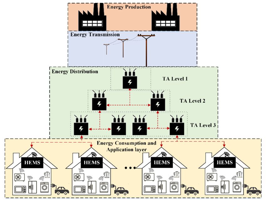
Sensors 2021, 21, 130                                                                                           2 of 16

                        article [8], the authors focus on scalability and acceptability where they categorized ap-
                        pliances, ordered their consumptions and defined boundaries for appliance usage time
                        slots to bound the consumption and to make the consumption diagram smooth. In [9],
                        the authors have clustered loads based on their priorities within a Neighborhood-Area
                        Network (NAN) with the goal to find a tradeoff between Energy Management System
                        (EMS) processing cost and response time delay to achieve demand-supply balance. Note
                        that in this paper, comfort is associated with improved fairness in delay and dispatch rates.
                        The authors in [10] have focused on minimizing the household bill based on different
                        categories of appliances and dynamic pricing tariff using Genetic Algorithm (GA) method
                        to find the optimal operating parameters for each individual device. Finally, in [11] they
                        have minimized the total energy cost of appliance rescheduling, treating rescheduling as
                        an inconvenience (that is, a discomfort).
                              With the increasing penetration of renewable energies at the residential level, some
                        of the previous works on demand side management have proposed appliance scheduling
                        based on the power available from renewable resources. A hierarchical model has been
                        proposed in [12] to maximize Distributed Energy Resource (DER) use and to reduce the
                        load on the grid. In this model, loads are bundled and scheduled to align their consumption
                        patterns with available renewable resources. This approach not only reduces the load on
                        the grid but also reduces customer cost. In [13], the authors have aimed to reduce the cost
                        while keeping the power consumption in a building under a certain threshold. For cost
                        minimization, they shared the DER power generated between all the residents. In [14], the
                        authors integrated a sensor network with a home energy management system and showed
                        that energy consumption can be reduced with a system that employs communication with
                        the users.
                              DSM can also utilize the predicted day-ahead load [15]. In [16], the authors have
                        performed day-ahead scheduling using real-time pricing by predicting next-day customer
                        demand. Their main goal is to accurately predict the load and minimize the cost of
                        generation. In this case, the authors have increased customer satisfaction using an incentive-
                        based model.
                              One of the important comfort factors at the residential level is the temperature of the
                        living area, which corresponds to the thermal load. The thermal load can be defined for
                        different devices, such as a HVAC system. Most of the studies in this area have tried to
                        minimize the thermal load while maintaining the customer’s comfort. In [17], authors have
                        scheduled HVAC energy consumption by increasing or decreasing the room’s temperature
                        under a price consideration. Thus, customer comfort is considered as an energy cost.
                        In several studies, authors have added other features addition to the thermal load to
                        improve their calculations [18,19]. In [18], the main goal was to minimize the HVAC’s
                        cost of energy and also to maintain customer comfort. In their work, the authors looked
                        for different parameters that affect room temperature, such as the number of occupants,
                        indoor and outdoor temperature, and customer preference. They used a nonconvex
                        formulation to solve their problem with tradeoff between cost and thermal comfort. The
                        work in [19] presented central demand management to control building Air Conditioner
                        (AC) power consumption and preferred temperature. This scheme evaluated the system
                        communication delay, outdoor temperature and other features. Meanwhile, the authors
                        in [20] proposed a MILP based on dynamic pricing to optimize the thermal load in a smart
                        house and to maintain customer comfort. In [21], the authors addressed HVAC system
                        energy conservation and wastage using a machine learning approach, using Internet of
                        Things (IoT) sensor data to establish consumer consumption patterns.
                              In several articles on thermal load management, the authors have taken a thermal
                        standard as index and addressed temperature in that context. In [22], authors used the
                        ISO standard on residence’s comfort temperature and minimized Predicted Percentage
                        Dissatisfaction (PPD). Then, they applied a direct load control model with Particle Swarm
                        Optimization (PSO) to reduce thermal load. Other approaches have optimized both thermal
                        and non-thermal loads to increase systems efficiencies, as noted in [23,24].
Sensors 2021, 21, 130                                                                                                 3 of 16

                                     Most of the papers in the DSM area use a mathematical model to minimize or maximize
                               one or many objective functions with different load constraints. For instance, the authors
                               in [25] have implemented a forecasting model to predict household renewable generation
                               and load, then they have applied an optimization model to schedule the appliance usage
                               profile based on increasing EV charging, reducing the total cost and maximizing the benefit
                               of selling renewable. The linear programming approach has been used in [26] to minimize
                               customer cost and constrain the total usage cost to be less than a specific budget. In
                               addition, a Mixed Integer Non-linear Programming (MINP) approach has been used in [27]
                               to control cost and appliances usage. The idea of using MILP in DSM is to find optimal time
                               slots (integer value) for load profiles. The multi-objective MILP in [28] has been presented
                               to control PAR, cost and schedule inconvenience using ToU tariff. In addition, several
                               works focus on appliance management. They have categorized such loads in different
                               categories and then apply a suitable objective function with proper constraints to schedule
                               them [29]. In [30,31], the authors have presented a prioritized model based on the appliance
                               categories to minimize their costs. For more clarification, we categorized the reviewed
                               articles in Table 1.

                                          Table 1. Categorizing the reviewed papers.

                             Objectives
                                                                                             Load              Load
    Paper                   Appliance      Thermal         Techniques         Real-Data
                    Cost                                                                    Category       Prioritization
                             Usage         Comfort
      [7]               4      4                               NLP                4            4                 4
                                                           ColorPower
      [8]               4      4                                                               4                 4
                                                            algorithm
      [9]               4      4                               NLP                             4                 4
     [10]               4      4                               GA                              4
     [11]               4      4                                LP                                               4
     [12]               4      4                          Minority Game           4                              4
     [13]               4                                      NLP
     [14]               4                                       LP
     [15]               4                                       LP                                               4
     [16]               4                                       LP
     [17]               4                     4                 LP                                               4
     [18]               4                     4            Non-convex
     [19]                                     4                DLC                4                              4
     [20]               4                     4               MILP                4
     [21]                                     4                ML                 4
     [22]                                     4                PSO
     [23]               4                     4                 LP                4
     [24]               4                     4                NLP
     [25]               4      4                                LP                4
     [26]               4                                       LP                                               4
     [27]               4      4                              MINP
     [28]               4      4                              MILP                4                              4
     [29]               4      4                                LP                                               4
                                                         Problem-Solving
     [30]               4      4                                                  4            4                 4
                                                            approach
     [31]               4                                     BPSO                                               4

                                    In this paper, we present a multi-objective sequential optimization model to distribute
                               loads over a time horizon. The loads are categorized into three clusters of load types
                               essential, deferrable and elastic, and for that reason we name our method as Clustered
                               Sequential Management (CSM). Our proposed approach considers a house with a Home
                               Energy Management System (HEMS) which is able to prioritize appliances and communi-
                               cate with the users. We use ToU pricing rates as the price signal. We propose MILP and
                               LP based optimization techniques that jointly minimizes the cost and maximize thermal
                               comfort. Our main contribution is a multi-objective model based on different types of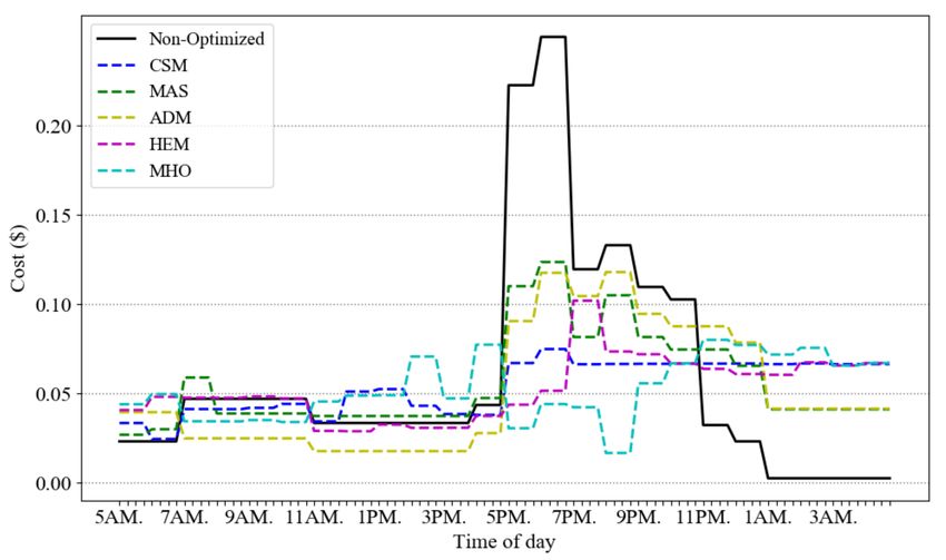
Sensors 2021, 21, 130                                                                                            4 of 16

                        appliances, different priorities of appliances, utility price signal vector over peak hours and
                        considering thermal satisfaction regarding to ASHRAE standard to maintain temperature
                        in a standard range and prevent wasting the energy for heating the house. The main
                        contribution of this work is employing both MILP and LP optimization models to reduce
                        customer energy bill and PAR by considering thermal comfort jointly with a prioritized
                        appliance scheduling. We considered a variety of load categories to assess the proposed
                        optimization methods including non-flexible (essential loads) as well as flexible loads (elas-
                        tic and deferrable loads). The proposed model has been validated in helping customers to
                        save their energy bill using a real appliances energy profiles.
                              The rest of the paper is organized as follows. Section 2 presents our system model and
                        the proposed optimization models. In Section 3, we illustrate our results, and in Section 4
                        we present our conclusions.

                        2. System Model and Problem Formulation
                             With the advances in smart appliances, home appliances are now a part of the IoT
                        ecosystem while the smart grid positions itself as an ideal example of an Industrial IoT
                        (IIoT) system [32]. Figure 1, illustrates the major elements of this ecosystem. At the top
                        level, we have generators that could be based on conventional or renewable energy sources.
                        Then, the produced energy is transported through transmission lines to the distribution
                        system transformers, which is called as transformer level. At energy distribution level,
                        each Transformer Agent (TA) will balance the voltage and frequency to be suitable for
                        residential usage by stepping up/down the voltage. At the residential level, HEMS, as an
                        IoT device, communicates with TA to send the customer’s usage data to the utility. The
                        household IoT devices (such as HVAC, EV, washing machine and etc.) communicate with
                        HEMS through Wi-Fi or Zigbee and create a small network inside the house.

                        Figure 1. Top-down view of our IoT ecosystem.

                              In this paper, we assume that the utility sends a Demand Response (DR) signal to
                        the customers and asks them to collaborate on demand management to manage the grid
                        supply and demand at peak times. However, customers have appliances that need to be on
                        during certain times and they also have thermal loads that can be controlled to maintain a
                        certain level of user satisfaction. To achieve these goals, a smart HEMS device is needed.
                        The device is able to control and monitor the customer’s power consumption. Our aim is
                        to minimize the cost, maximize the customer’s comfort and to reduce the PAR based on
                        utility’s DR signal.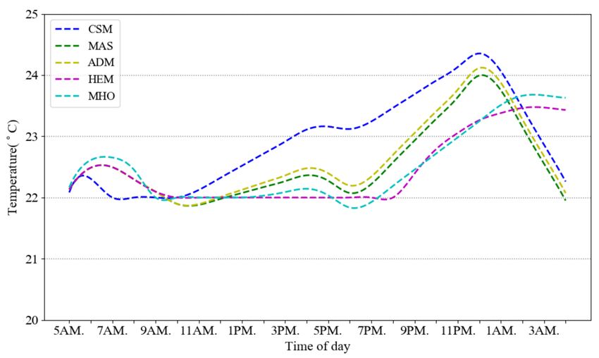
Sensors 2021, 21, 130                                                                                               5 of 16

                            Let N be the number of customers, where i ∈ N is the customer index. Subscript
                        a denotes the appliance number and Ai is the set of appliances for customer i, where
                        a ∈ Ai . The number of appliances for customer i is given by |Ai |. We subdivide the
                        24-hour period into T equal time slots and t ∈ {1, 2, . . . , T}. An appliance
                                                                                                h      profile
                                                                                                           i may be
                        defined in terms of its nominal pattern of power consumption La = la1 , · · · , laTa , where lat
                        is the appliance energy consumption in time slot t, and the dimensionality is expressed by
                        the number of time slots Ta over which the appliance operates.           Its optimized operating
                        state during the day is given by the binary vector τa = τa1 , · · · , τaT , where the appliance


                        condition (ON/OFF) for time slot t is given by τat (i.e., 1 or 0). This operating state is
                        determined by  a scheduling       and optimization process (described below) that transforms
                        La into Xa = x1a , · · · , xTa , where x ta is the optimized appliance consumption for time slot t.


                        The customer aggregated load vector χi = [χ1i , . . . , χTi ] is sequentially constructed, with χit
                        the total optimized load for time slot t.

                        2.1. Load Categories and Scheduling Approach
                             We consider three load categories. Essential loads (AE ) are those directly initiated
                        by the user, lacking any HEMS control of their power consumption or profile (e.g., coffee
                        maker). Elastic loads (AEl ) are those with load profiles whose consumption may be
                        adjusted by HEMS control within any time interval (e.g., HVAC). Such loads have a central
                        impact on customer comfort level. Deferrable loads (AD ) are those whose load profiles are
                        schedulable (e.g., washing machine) within some customer-defined interval. Such loads
                        have a central impact on customer         lifestyle and convenience. For each appliance a, we
                        define a binary vector Ia = Ia1 , · · · , IaT , where


                                                                   (
                                                                       1   ts ≤ t ≤ t f
                                                        Iat   =                               , ∀ Iat ∈ Ia             (1)
                                                                       0   otherwise

                        denotes the permissible scheduling interval in terms of starting and finishing time slots ts
                        and t f , respectively. This permits time constraints to be set. One fundamental constraint is
                        that the permissible interval be greater than the usage time Ta , where

                                                                           t f − ts > Ta                               (2)

                             Ai is composed of distinct subsets and may be represented as:

                                                                   Ai = {AE , AEl , AD }.                              (3)

                               Appliances may also be categorized by their usage priority, with essential loads being
                        mandatory. For all other loads, priority levels are customer-assigned via the HEMS, but
                        elastic loads are assumed to have a higher priority than deferrable ones. The appliances
                        priority is denoted by Γi = [ρ1 , . . . , ρM ] with length of M = |AEl | + |AD |, whose element
                        ρ a is appliance a priority coefficient. To allocate the priority coefficients to these appliances,
                        we use the Analytic Hierarchy Process (AHP) [33] in our optimization model.
                               We implement load optimization, described in the following subsection, within a se-
                        quential approach. This is illustrated in the flowchart provided in Figure 2. This sequential
                        scheduling considers the appliance load profiles entered into the load vector by order of
                        priority. Note that the summation of χi across the time horizon should be almost equal to
                        the summation of all the appliances’ load profiles:

                                                                               | Ai | T a
                                                                                                  !
                                                               T
                                                              ∑      χit   =   ∑∑           lat       ± ∆.             (4)
                                                              t =1             a =1 t =1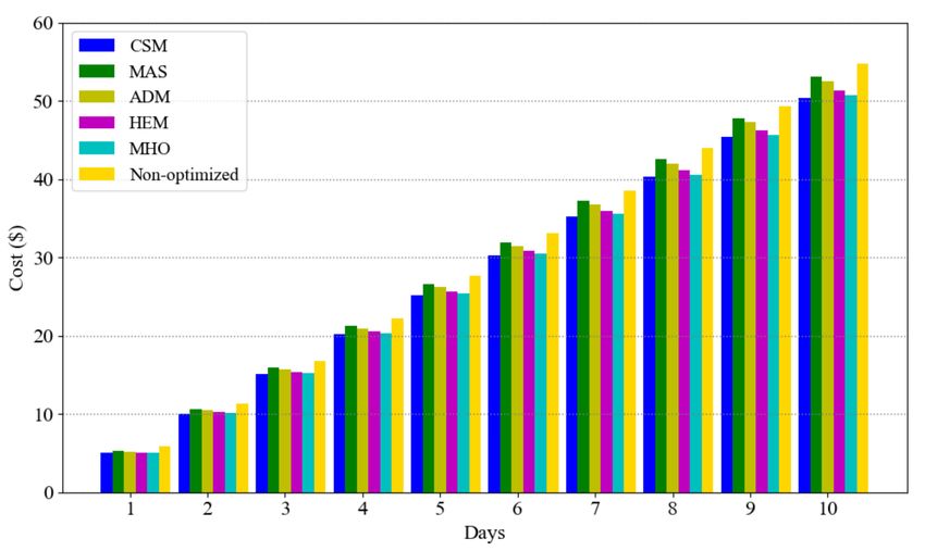
Sensors 2021, 21, 130                                                                                           6 of 16

                        Figure 2. The flowchart of our proposed model.

                        2.2. Optimization
                             The ultimate goal of the proposed optimization scheme is to minimize the total
                        residential energy consumption which is given by min f (xa ) + g(xa , τa ). Each appliance is
                        contributing to this optimization model by minimizing their own consumption as explained
                        below. Constraints specific to appliances type, essential, elastic or deferrable, are applied.
                        We optimize Xa and τa by sequentially minimizing the cost of        the incremented    daily
                        load, χi ← Xa + χi , using a general time-of-use price signal P = p1 , · · · , pT .


                        2.2.1. Elastic Load Model
                             Elastic devices have a defined operating state τa (i.e., are not schedulable) but their
                        power consumption xa is adjustable. By considering the general form of optimization, we
                        can define an LP optimization model for this category as

                                                                    tf
                                                 min f (xa ) = min ∑ pt x ta + χit

                                                                   t=ts
                                                           tf
                                                 Subj.to β ∑ log x ta + 1 ≥ Sa

                                                                                                                   (5)
                                                          t=ts                     h         i
                                                         (1 − β)PPD x ta ≤ Da , t ∈ ts , t f


                                                         χit ≤ x ta + χit ≤ Ubt

                        where pt is ToU pricing signal; x ta ∈ Xa is appliance a consumption for time slot t; χit ∈ χi
                        is the aggregated load vector of customer i at time slot t; and ts and t f are the appliance’s
                        preferred starting and finishing work time intervals, respectively. If the appliance is a
                        non-thermal elastic load, β = 1(such as EV), otherwise β = 0 (such as HVAC). The first
                        constraint is specifically used for non-thermal loads, where Sa is the minimum level of
                        power consumption extracted as in [34]. A logarithmic function is used to ensure minimum
                        device performance in the limit as such a function saturates [35]. The second constraint is
                        used for the thermal system and depends on environment and appliance energy dissipation.
                        Da is the threshold for Predicted Percentage Dissatisfaction (PPD) to ensure customer’s
                        dissatisfaction remains less than a certain value. We use PPD function to measure the
                        customer’s dissatisfaction regarding room temperature [36]. PPD is defined in the ASHRAE
                        standard and it is governed by the parameters that establish room conditions. There is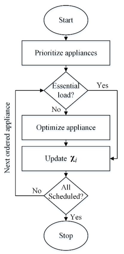
Sensors 2021, 21, 130                                                                                             7 of 16

                        an indirect relation between PPD and power consumption using Predicted Mean Vote
                        (PMV) [17,37]. Finally, the third constraint is used for both thermal and non-thermal loads
                        to bound each time slot between the aggregated load χit and the maximum threshold of
                        household usage Ubt ∈ Ub at time slot t. The goal of defining a limitation for each time
                        slot is to prevent peak events and distribute the customer load evenly throughout the day.

                        2.2.2. Deferrable Load Model
                             In the case of deferrable load scheduling, the optimization model will manage the
                        load profile through the permissible interval and find the minimum cost. This approach is
                        completely different than the previous model for elastic devices. In this model, instead of
                        LP, we are using MILP. This model helps us to first find the proper time for appliance usage
                        and then find the optimized load profile vector for appliance a. For this optimization, as a
                        general model we have
                                                                     tf
                                                ming(xa , τa ) = min ∑ pt τat x ta + χit ,

                                                                           t=ts
                                                         tf
                                                Subj.to ∑ τat Iat = Ta
                                                        t=ts                                                         (6)
                                                           k +T a
                                                              ∑    pk x ka ≤ Ca , ts ≤ t ≤ t f − Ta
                                                        τat =1⇒k =t
                                                          χit ≤ τat x ta + χit ≤ Ubt


                        where pt is ToU pricing signal; x ta ∈ Xa is the appliance a consumption at time slot t;
                        χit ∈ χi is the aggregated load of customer i at time slot t; τat ∈ τa is the operating state
                        of appliance a (the ON/OFF condition) at time slot t; and ts and t f are the appliance’s
                        starting and finishing work time intervals, respectively. The first constraint is used to find
                        Ta , which is the number of time slots the appliance needs to complete its operation within
                        the permissible interval Ia ( Iat ∈ Ia ). The second constraint is used to require uninterrupted
                        device operation, with Ca the minimum operation cost for appliance a in its permissible
                        interval; τat = 1 ⇒ k = t ensures that if and only if the optimized operating state is equal
                        to one, then the time slot and the summation of cost for the Ta time slots after that (from
                        k = t to k + Ta ) should be lower than or equal to the minimum cost Ca . The third constraint
                        is used to bound each time slot between the aggregated load vector and the maximum
                        threshold of household usage at time slot t.

                        2.3. Thermal Model
                              As mentioned in Section 2.2.1, we choose a PPD rate and with PPD and PMV functions
                        we calculate the necessary thermal load [17]. To make a map between PPD, PMV, thermal
                        energy and temperature, we consider the fundamentals of thermal conduction. Room
                        size, wall quality and inside and outside temperatures have direct impact on thermal loss.
                        From [38],
                                                                            dθroom
                                                          Q power = Croom ×                                         (7)
                                                                              dt
                        is used to calculate the thermal power needed to change
                                                                                the room temperature θ Inside to the
                        preferred temperature θ pre f erred at a specific rate dθdt
                                                                                 room
                                                                                      , where Croom is the room thermal
                        capacity [38]. The power leakage is determined via

                                                                        θOutside − θ Inside
                                                              Qleak =                       ,                        (8)
                                                                                R
                        where θOutside is the outdoor temperature and R is the room’s thermal resistance. In our
                        model we are using both formulations with regard to ASHRAE standard room temperature.
                             Figure 3 shows that when PPD is equal to 11.68%, we need to consume almost 1.8 kWh
                        to increase the room’s temperature from 20 °C to 22.5 °C when the outside temperature
                        is −10 °C. According to the ASHRAE standard [36], the optimal temperature range for a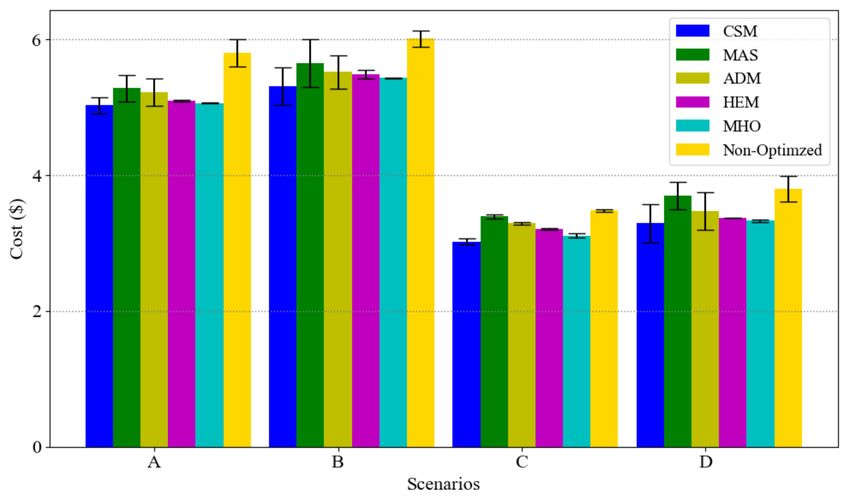
Sensors 2021, 21, 130 8 of 16
room in winter with the optimal PPD (≤10%) is between 23 °C and 27 °C which is also
observable from Figure 3. Therefore, our algorithm tries to keep the temperature in this
range regarding to room heating leakage, outside temperature and inside temperature.
Figure 3. Relation between PPD, PMV, temperature and energy [Assumption:θOutside = −10 °C].
2.4. Analytic Hierarchy Process (AHP)
AHP is a decision-making model that is used for ranking the alternatives when we
have multi-criteria problems [33]. A pairwise comparison is made between the specified
criteria and alternatives with the grades ranging from 1 to 9. The value r ∈ {1, . . . , 9}
shows how much more priority an alternative have over the other. Intensity r = 1 means
they are equal, r = 2, 3 shows the moderate condition, r = 4, 5 means one is stronger than
the other, r = 6, 7 one is very strong and r = 8, 9 presents the extreme importance of one to
the other. Let’s assume we have m criteria and n alternatives then, the relative matrix Ak
for criteria k (k ∈ {1, . . . , m}) represents the relative rates between alternatives i and j (αij )
where i, j ∈ {1, . . . , n} and it is calculated by αij = rri where ri , r j ∈ {1, . . . , 9}.
j
r1 r1
α11 α12 . . . α1n
1 r2
... rn
r2 r2
α21 α22 . . . α2n
r1 1 ... rn
Ak = = (9)
.. .. . . .. .. .. .. .
. . . . . ..
. .
. . . αnn rn rn
αn1 αn2 r1 r2 ... 1
αij
After filling the matrix, we normalize each relative rate αij using αij = ∑in=1 αij
and to
∑nj=1 αij
calculate the alternative i’s weight in criteria k, we have wik = n . Then, we extend
matrix Ak for other criteria and calculates wik , ∀ i ∈ {1, . . . , n}, k ∈ {1, . . . , m}. After that,
we rate the criteria relatively in the same way and multiply the criteria weight wk with
each alternative weight wik and finally the alternative i’s priority will be calculated using
m
ρi = ∑ (wk × wik ).
k =1
In our model, we have implemented a two-level AHP to fairly prioritize the appliances
in our sequential optimization model. We have two criteria (m = 2), customer preferences
on appliance usage and appliance total consumption, and 6 deferrable and elastic loads
as alternatives (n = 6). There might be other criteria and alternatives, but in our case we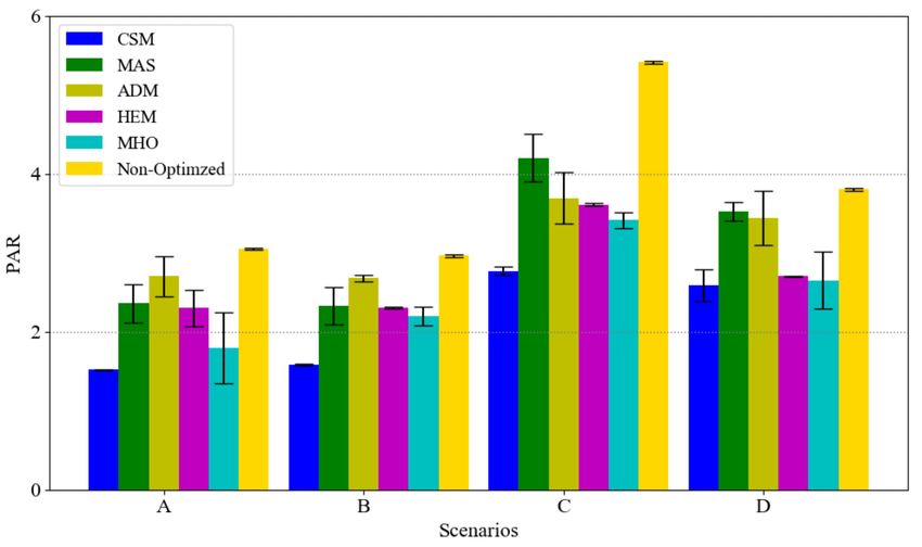
Sensors 2021, 21, 130                                                                                              9 of 16

                        found that these are the most important ones that affect appliances scheduling. In our
                        model, the AHP algorithm is implemented in HEMS. Then, each customer can interact with
                        HESM and rate each two appliances relatively. Note that HEMS has the total consumption
                        information of connected appliances. Finally, HEMS does the AHP computation and find
                        the appliances weight or priority values.

                        3. Simulation Results
                             In this section, we present our simulation results and compare our model, Clus-
                        tered Sequential Management (CSM), with four other demand management approaches;
                        Multi-class Appliances Scheduling (MAS) [34], Autonomous Demand-side Management
                        (ADM) [39], Household Energy Management (HEM) [10], and Multi-objective Household
                        appliance Optimization (MHO) [28]. To make our implementation close to real world
                        conditions, we use the dataset of household appliances load profile from [40]. Table 2
                        presents the appliances’ type and their total power consumption in a day.

                        Table 2. Types of appliances.

                                   Appliance                       Load Type                    Energy (kW/day)
                                   Heater                           Elastic                           25.43
                                     EV                             Elastic                             26
                                   Freezer                         Deferrable                         2.07
                               Washing Machine                     Deferrable                          1.96
                                 Cloth Dryer                       Deferrable                          2.47
                                Dish Washer                        Deferrable                          1.44
                                 Refrigerator                      Essential                           3.65
                                Coffee Maker                       Essential                           0.19
                                     TV                            Essential                           2.57
                                    Light                          Essential                           0.41
                                    Stove                          Essential                          0.61
                                      PC                           Essential                          3.93

                               The simulation environment is Python and we use SciPy library to solve MILP and
                        LP optimization models. This simulation is conducted on Intel i5 CPU with 3.55 GHz
                        clock speed and 16 GB RAM. Also, our algorithm processing time was 10 seconds. Four
                        different scenarios with different mixes of appliances are used for performance evaluation.
                        These are indicated in Table 3 and are comprised of (i) 6 essential, 2 elastic (EV and Heater)
                        and 1 deferrable loads, (ii) 5 essential, 2 elastic (EV and Heater) and 2 deferrable loads,
                        (iii) 4 essential, 1 elastic (EV) and 3 deferrable loads, and (iv) 3 essential, 1 elastic (Heater)
                        and 4 deferrable loads. These are defined to compare the sensitivity and effectiveness of
                        five different approaches (CSM, MAS, ADM, HEM and MHO) with respect to load types.
                        Note that other combination of loads do not impact the workings of the proposed scheme.
                        Therefore we choose these four different scenarios to evaluate the performance of our
                        model. In MAS and ADM, all the power consumption is accumulated and distributed
                        through the permissible intervals without considering the appliances’ priority on power
                        consumption and customer’s preferences. However in MAS, the authors categorize the
                        appliances into different load clusters and optimize each using their specific optimization
                        function. Moreover, in MAS deferrable loads are non-interruptible. Also, we compare our
                        model with other recent articles HEM and MHO. They have some similarities with our
                        model in comfort, cost minimization and appliance scheduling. Besides these similarities,
                        there are some differences. In HEM [10], the authors have implemented an iterating GA
                        and assumed different load categories with different settings to adjust appliance time usage
                        and comfort level. However the loads are optimized simultaneously without considering
                        the essential load effects on peak and cost. On the other hand, in MHO [28], their multi-
                        objective model focused on minimizing cost, peak, and scheduling inconvenient. The
                        authors determined different orders of these three factors and again optimize all the
Sensors 2021, 21, 130 10 of 16
appliances simultaneously with many constraints. In [28] the effect of the essential loads
on the peak consumption and cost has not been considered.
Table 3. Load profile scenarios.
Load Type
Essential Elastic Deferrable Total Energy
Scenarios
(kW/day)
Qty. Pct. Qty. Pct. Qty. Pct.
Scenario A 6 17.7% 2 80.1% 1 2.2% 64.23
Scenario B 5 16.9% 2 77.8% 2 5.3% 66.11
Scenario C 4 18.5% 1 66.5% 3 15% 39.11
Scenario D 3 16.6% 1 63.6% 4 19.8% 40
To put the appliances in order for our sequential optimization, or in another words, to
prioritize them, we used the AHP method which is explained in Section 2.4. This yielded
the priority vector Γi = [ρ1 , . . . , ρM ] for M deferrable and elastic devices. Note that in
this model, elastic loads have higher priority than deferrable ones because their total
consumption is higher than deferrable loads.
In this simulation, scheduling is performed across a 24-h day subdivided into 96
equal time slots beginning at 5 AM. We use a ToU pricing signal based on the Ontario
Energy Board (OEB) [41], with household energy consumption based on an average winter
consumption in Ontario, Canada. We assume the customer wants to keep the room
temperature within the maximum permissible ASHRAE standard range and we include
provisioning for fully charging an EV. We consider a room size of 118.4 square feet, with
θOutside = −10 °C (the average outside temperature in December 2018 in Ontario), and an
inside temperature of θ Inside = 22 °C. We assume a PPD of less than 16%.
Figure 4 presents the optimized power consumption of scenario A in six different
models: our CSM, versus MAS, ADM, HEM, MHO and the non-optimized case. Note that
for MHO implementation, we choose the order of inconvenient, cost and peak optimization
(scenario 3 in [28]) which is closer to our proposed architecture. This figure shows the
average result of 10 runs. The price signal presents different tiers of ToU pricing (off-peak,
mid-peak and on-peak). As observed from the figure, the proposed model reduces the
peak consumption almost 30% more than the MAS, ADM and HEM, and 15% more than
MHO in scenario A.
Figure 4. ToU rate and average energy consumption scheduling in a day of scenario A.Sensors 2021, 21, 130 11 of 16
Figure 5 gives the cost profiles for the load demands of Figure 4. Due to the flattening
impact of our CSM scheme, its overall cost is lower than the other schemes. Figure 6
illustrates how the temperature is fluctuating over different time slots in the compared
approaches. The five models are consuming the same amount of power in a day to keep
the room warm but their temperature is different on different time slots. Our approach is
keeping the temperature in ASHRAE standard range and increasing the temperature close
to 25 °C which is the best room temperature in winter. The approaches MAS, ADM and
MHO schedule the total energy regardless of thermal comfort formulation but consuming
the same minimum range of electricity for thermal load during a day.
Figure 5. Cost changes in different time slots for five models.
Figure 6. Temperature fluctuation in different models.
But HEM model has a thermal constraint for setting the minimum and maximum room
temperature. Here we set it between 22 °C and 25 °C same as our model assumption. CSM
and HEM keeps the temperature more than 22 °C but our model increases the temperature
more (close to 24.35 °C) to reduce the PPD. Table 4 is a summary of the minimum and
maximum temperatures and the averaged PPD in a day for the different approaches. Our
CSM approach has the lowest PPD and though it does have a slightly greater temperature
excursion than the other approaches, while still remaining within the limits, the rate ofSensors 2021, 21, 130 12 of 16
temperature variation is much less. HEM has higher PPD than MHO despite of having
temperature constraint. The HEM guarantees to keep the temperature in the comfort
range (more than 22 °C) and minimize the bill. Therefore, at peak times it consumes the
minimum electricity which is needed to satisfy the temperature constraint. But MHO
is fluctuating through the times and cooling and warming the house based on the ToU
pricing signal.
Table 4. Results comparison.
Approach PPD (%) Tmin (°C) Tmax (°C)
CSM 11.68 22 24.35
MAS 13.83 21.88 23.99
ADM 13.37 21.89 24.11
HEM 14.27 22 23.46
MHO 13.99 21.83 23.66
As a consequence, the best way for simulating a household thermal comfort is to use
a standard satisfaction formulation such as PPD in optimization constraint instead of only
considering the temperature range.
To ensure that our approach is robust with regard to parameter choice, we repeat
scenario A for 10 days and calculate the cumulative cost for different approaches; the results
are presented in Figure 7. Our approach is seen to always have less cost than the others.
The reason that MAS has higher cost than ADM is that, in the former, the deferrable loads
are non-interruptible which constrains usage time but in the latter they are interruptible
and unconstrained. Also, HEM and MHO have almost more accumulated cost than CSM
which is due to the lack of essential load consideration on their scheduling. Moreover, we
can assert that within 10 days of consumption, customer saves almost $5 and if we extend it
to a month the saving would be $15. Note that the average cost of electricity bill in Ontario,
Canada is $125 per month [41]. Therefore, the customer’s savings would be considerable.
Figure 7. Cumulative cost in 10 days.
To present the effect of load clustering and prioritization on our model, Figures 8 and 9
present the results of different scenarios on the total cost and PAR, respectively. Note that,
in each scenario, the total power demand is equal between the six approaches.Sensors 2021, 21, 130 13 of 16
Figure 8. Total cost in a winter day on different scenarios with confidential interval.
Figure 9. PAR on different scenarios with confidential interval.
Based on Figure 8, our model has the lowest cost in all the scenarios considered.
The appliances’ usage priority cause that elastic loads, with the high consumptions, are
optimized first and then the prioritized deferrable loads optimized in next level. Moreover,
considering essential loads usage as a lower bound in optimization model helps to reduce
the total cost either.
Regarding to Figure 9, the PAR in our model is the minimum one and the reason why
ADM has less PAR than MAS in scenarios C and D is due to the interruptible deferrable
load assumption in ADM model (in scenario C and D number of deferrable loads are
increased). Moreover, HEM and MHO has less PAR than ADM and MAS, because of their
optimization models, GA and MILP. Also, it shows that the appliance usage priority and
clustering have positive effects on finding proper time slots for the appliances consumption
especially for the elastic load with high demand. Finally, we can assert that we reduced the
cost almost 8%, 6%, 5% and 3%, and reduced PAR almost 34%, 33%, 24% and 17% more
than MAS, ADM, HEM and MHO respectively.
4. Conclusions
In this paper we have presented a multi-objective demand management approach
using appliance clustering and prioritization, and keeping the customer’s thermal comfortSensors 2021, 21, 130 14 of 16
in ASHRAE standard range. Customer’s comfort is considered in many aspects, prioritizing
appliances for the sequential optimization (the one optimized first will completely satisfy all
its constraints), customer’s comfort on thermal load, EV’s state of charging, and deferrable
loads’ non-interruptible usage on selected permissible time interval.
Our main goals are to flat the household demand and effectively reduce the customer’s
cost while increasing customer comfort via their elastic and deferrable loads. In this work,
we compared our light-weight model with other demand management methods, which
have similarities in prioritization, clustering, PAR and cost management. Our results
represent that we smoothed the load profile and reduced PAR almost 45% more than the
non-optimized case, decreased the electricity bill almost 13%, keep the room’s temperature
in ASHRAE standard range and charge EV more than the customer’s desired amount.
Author Contributions: The authors contributed equally to conceptualization and methodology.
Software, validation, writing—original draft preparation, M.S. Validation, J.F. Writing—review and
editing, supervision, M.E.-K. and H.S. All authors have read and agreed to the published version of
the manuscript.
Funding: This research is funded in part by NSERC CREATE under grant number 497981, by NSERC
CRDPJ 477238-14 and by Hydro Ottawa.
Institutional Review Board Statement: Not applicable.
Informed Consent Statement: Not applicable.
Data Availability Statement: Data sharing not applicable.
Conflicts of Interest: The authors declare no conflict of interest.
Abbreviations
Acronym Description
AC Air Conditioner
AHP Analytic Hierarchy Process
ADM Autonomous Demand-side Management
BPSO Binary Particle Swarm Optimization
CSM Clustered Sequential Management
DER Distributed Energy Resource
DR Demand Response
DSM Demand Side Management
EMS Energy Management System
GA Genetic Algorithm
GHG Greenhouse Gas
HEM Household Energy Management
HEMS Home Energy Management System
HVAC Heating Ventilation and Air Conditioner
IIoT Industrial IoT
IoT Internet of Things
LP Linear Programming
MAS Multi-class Appliances Scheduling
MHO Multi-objective Household appliance Optimization
MILP Mixed Integer Linear Programming
MINP Mixed Integer Non-linear Programming
ML Machine Learning
NAN Neighborhood-Area Network
NLP Non-linear Programming
OEB Ontario Energy Board
PAR Peak-to-Average Ratio
PMV Predicted Mean Vote
PPD Predicted Percentage Dissatisfaction
PSO Particle Swarm Optimization
TA Transformer Agent
ToU Time of UseSensors 2021, 21, 130 15 of 16
References
1. Torriti, J. Price-based demand side management: Assessing the impacts of time-of-use tariffs on residential electricity demand
and peak shifting in Northern Italy. Energy 2012, 44, 576–583. [CrossRef]
2. Samadi, P.; Mohsenian-Rad, H.; Schober, R.; Wong, V.W.S. Advanced demand side management for the future smart grid using
mechanism design. IEEE Trans. Smart Grid 2012, 3, 1170–1180. [CrossRef]
3. Kinhekar, N.; Padhy, N.P.; Gupta, H.O. Multiobjective demand side management solutions for utilities with peak demand deficit.
Int. J. Electr. Power Energy Syst. 2014, 55, 612–619. [CrossRef]
4. Lampropoulos, I.; Kling, W.L.; Ribeiro, P.F.; Berg, J.V.D. History of demand side management and classification of demand
response control schemes. In Proceedings of the 2013 IEEE Power & Energy Society General Meeting, Vancouver, BC, Canada,
21–25 July 2013.
5. Pourbabak, H.; Chen, T.; Su, W. Centralized, decentralized, and distributed control for Energy Internet. In The Energy Internet;
Elsevier: Amsterdam, The Netherlands, 2019; pp. 3–19.
6. Yaghmaee, M.H.; Kouhi, M.S.; Garcia, A.L. Personalized pricing: A new approach for dynamic pricing in the smart grid. In
Proceedings of the 2016 IEEE Smart Energy Grid Engineering (SEGE), Oshawa, ON, Canada, 21–24 August 2016; pp. 46–51.
[CrossRef]
7. Liu, Y.; Yuen, C.; Yu, R.; Zhang, Y.; Xie, S. Queuing-based energy consumption management for heterogeneous residential
demands in smart grid. IEEE Trans. Smart Grid 2016, 7, 1650–1659. [CrossRef]
8. Ali, S.M.; Naveed, M.; Javed, F.; Arshad, N.; Ikram, J. DeLi2P-A user centric, scalable demand side management strategy for
smart grids. In Proceedings of the 4th International Conference on Smart Cities and Green ICT Systems, Lisbon, Portugal, 20–22
May 2015; pp. 148–156.
9. Tahir, M.; Mazumder, S.K. Event-and priority-driven coordination in next-generation grid. IEEE J. Emerg. Sel. Top. Power Electron.
2016, 4, 1186–1194. [CrossRef]
10. Jiang, X.; Xiao, C. Household energy demand management strategy based on operating power by genetic algorithm. IEEE Access
2019, 7, 96414–96423. [CrossRef]
11. Alam, M.R.; St-Hilaire, M.; Kunz, T. Cost optimization via rescheduling in smart grids; A linear programming approach. In
Proceedings of the 2013 IEEE International Conference on Smart Energy Grid Engineering (SEGE), Oshawa, ON, Canada, 28–30
August 2013; pp. 1–6.
12. Karthikeyan, R.; Parvathy, A.K. Real time energy optimization using cyber physical controller for micro-smart grid applications.
In Proceedings of the 2016 International Conference on Recent Trends in Information Technology (ICRTIT), Chennai, India, 8–9
April 2016; pp. 1–6.
13. Arun, S.L.; Selvan, M.P. Intelligent residential energy management system for dynamic demand response in smart buildings.
IEEE Syst. J. 2018, 12, 1329–1340. [CrossRef]
14. Erol-Kantarci, M.; Mouftah, H.T. Wireless sensor networks for cost-efficient residential energy management in the smart grid.
IEEE Trans. Smart Grid 2011, 2, 314–325. [CrossRef]
15. Sinha, A.; De, M. Load shifting technique for reduction of peak generation capacity requirement in smart grid. In Proceedings of
the 2016 IEEE 1st International Conference on Power Electronics, Intelligent Control and Energy Systems (ICPEICES), Delhi,
India, 4–6 July 2016; pp. 1–5.
16. Tumuluru, V.K.; Tsang, D.H.K. A two-stage approach for network constrained unit commitment problem with demand response.
IEEE Trans. Smart Grid 2016, 9, 1175–1183. [CrossRef]
17. Vasudevan, J.; Swarup, K.S. Price based Demand Response strategy considering load priorities. In Proceedings of the 2016 IEEE
6th International Conference on Power Systems (ICPS), New Delhi, India, 4–6 March 2016; pp. 1–6.
18. Yu, L.; Xie, D.; Huang, C.; Jiang, T.; Zou, Y. Energy optimization of HVAC systems in commercial buildings considering indoor air
quality management. IEEE Trans. Smart Grid 2018, 10, 5103–5113. [CrossRef]
19. Zhang, Y.; Lu, N. Demand-side management of air conditioning cooling loads for intra-hour load balancing. In Proceedings of
the 2013 IEEE PES Innovative Smart Grid Technologies Conference (ISGT), Washington, DC, USA, 24–27 February 2013; pp. 1–6.
20. Wang, H.; Meng, K.; Luo, F.; Dong, Z.Y.; Verbič, G.; Xu, Z.; Wong, K.P. Demand response through smart home energy management
using thermal inertia. In Proceedings of the 2013 Australasian Universities Power Engineering Conference (AUPEC), Hobart,
TAS, Australia, 29 September–3 October 2013; pp. 1–6.
21. Raza, R.; Hassan, N.U.; Morstyn, T. Determination of consumer behavior based energy wastage using IoT and machine learning.
Energy Build. 2020, 220, 110060. [CrossRef]
22. Guo, W.; Zheng, Y.; Wen, J.; Luo, F. Peak Load Reduction by Thermostatically Controlled Load Dispatch with Thermal Comfort
Model. In Proceedings of the 10th International Conference on Advances in Power System Control, Operation & Management
(APSCOM 2015), Hong Kong, China, 8–12 November 2015; p. 72.
23. Tasdighi, M.; Ghasemi, H.; Rahimi-Kian, A. Residential microgrid scheduling based on smart meters data and temperature
dependent thermal load modeling. IEEE Trans. Smart Grid 2014, 5, 349–357. [CrossRef]
24. Kyoho, R.; Goya, T.; Mengyan, W.; Senjyu, T.; Yona, A.; Funabashi, T.; Kim, C.-H. Optimal operation of thermal generating units
and smart houses considering transmission constraints. In Proceedings of the 2013 IEEE 10th International Conference on Power
Electronics and Drive Systems (PEDS), Kitakyushu, Japan, 22–25 April 2013; pp. 1225–1230.Sensors 2021, 21, 130 16 of 16
25. Lujano-Rojas, J.M.; Monteiro, C.; Dufo-López, R.; Bernal-Agustín, J.L. Optimum residential load management strategy for real
time pricing (RTP) demand response programs. Energy Policy 2012, 45, 671–679. [CrossRef]
26. Arun, S.L.; Selvan, M.P. Dynamic demand response in smart buildings using an intelligent residential load management system.
IET Gener. Transm. Distrib. 2017, 11, 4348–4357. [CrossRef]
27. Huang, G.; Yang, J.; Wei, C. Cost-Effective and Comfort-Aware Electricity Scheduling for Home Energy Management System.
In Proceedings of the 2016 IEEE International Conferences on Big Data and Cloud Computing (BDCloud), Social Computing
and Networking (SocialCom), Sustainable Computing and Communications (SustainCom) (BDCloud-SocialCom-SustainCom),
Atlanta, GA, USA, 8–10 October 2016; pp. 453–460.
28. Yahia, Z.; Pradhan, A. Multi-objective optimization of household appliance scheduling problem considering consumer preference
and peak load reduction. Sustain. Cities Soc. 2020, 55, 102058. [CrossRef]
29. Rasheed, M.B.; Javaid, N.; Ahmad, A.; Awais, M.; Khan, Z.A.; Qasim, U.; Alrajeh, N. Priority and delay constrained demand side
management in real-time price environment with renewable energy source. Int. J. Energy Res. 2016, 40, 2002–2021. [CrossRef]
30. Ihsane, I.; Miègeville, L.; Ait-Ahmed, N.; Guerin, P. Real-time management model for residential multi-class appliances. In
Proceedings of the 2017 IEEE PES Asia-Pacific Power and Energy Engineering Conference (APPEEC), Bangalore, India, 8–10
November 2017; pp. 1–6.
31. Shah, S.; Khalid, R.; Zafar, A.; Hussain, S.M.; Rahim, H.; Javaid, N. An Optimized Priority Enabled Energy Management System
for Smart Homes. In Proceedings of the 2017 IEEE 31st International Conference on Advanced Information Networking and
Applications (AINA), Taipei, Taiwan, 27–29 March 2017; pp. 1035–1041.
32. Aazam, M.; Zeadally, S.; Harras, K.A. Deploying Fog Computing in Industrial Internet of Things and Industry 4.0. IEEE Trans.
Ind. Inform. 2018, 14, 4674–4682. [CrossRef]
33. Saaty, T.L. Decision making with the analytic hierarchy process. Int. J. Serv. Sci. 2008, 1, 83. [CrossRef]
34. Lee, J.-W.; Lee, D.-H. Residential electricity load scheduling for multi-class appliances with Time-of-Use pricing. In Proceedings
of the 2011 IEEE GLOBECOM Workshops (GC Wkshps), Houston, TX, USA, 5–9 December 2011; pp. 1194–1198.
35. Tudoroiu, R.-E.; Zaheeruddin, M.; Radu, S.-M.; Tudoroiu, N. Real-time implementation of an extended Kalman filter and a PI
observer for state estimation of rechargeable Li-Ion batteries in hybrid electric vehicle applications—A case study. Batteries 2018,
4, 19. [CrossRef]
36. ANSI/ASHRAE Standard 55. Thermal Environmental Conditions for Human Occupancy; American Society of Heating, Refrigerating
and Air-conditioning Engineering: Atlanta, GA, USA, 2010.
37. Orosa, J.A.; Oliveira, A.C. A new thermal comfort approach comparing adaptive and PMV models. Renew. Energy 2011, 36,
951–956. [CrossRef]
38. Wilson, M.B.; Luck, R.; Mago, P.J. A first-order study of reduced energy consumption via increased thermal capacitance with
thermal storage management in a micro-building. Energies 2015, 8, 12266–12282. [CrossRef]
39. Mohsenian-Rad, A.-H.; Wong, V.W.S.; Jatskevich, J.; Schober, R.; Leon-Garcia, A. Autonomous demand-side management based
on game-theoretic energy consumption scheduling for the future smart grid. IEEE Trans. Smart Grid 2010, 1, 320–331. [CrossRef]
40. Reinhardt, A.; Baumann, P.; Burgstahler, D.; Hollick, M.; Chonov, H.; Werner, M.; Steinmetz, R. On the accuracy of appliance
identification based on distributed load metering data. In Proceedings of the 2012 Sustainable Internet and ICT for Sustainability
(SustainIT) Conference, Pisa, Italy, 4–5 October 2012; pp. 1–9.
41. Electricity Rates. Ontario Energy Board. Available online: https://www.oeb.ca/rates-and-your-bill/electricity-rates (accessed
on 2 April 2018).You can also read