Deriving Arctic 2 m air temperatures over snow and ice from satellite surface temperature measurements
←
→
Page content transcription
If your browser does not render page correctly, please read the page content below
The Cryosphere, 15, 3035–3057, 2021
https://doi.org/10.5194/tc-15-3035-2021
© Author(s) 2021. This work is distributed under
the Creative Commons Attribution 4.0 License.

Deriving Arctic 2 m air temperatures over snow and ice from
satellite surface temperature measurements
Pia Nielsen-Englyst1,2 , Jacob L. Høyer2 , Kristine S. Madsen2 , Rasmus T. Tonboe2 , Gorm Dybkjær2 , and
Sotirios Skarpalezos2
1 1DTU-Space,    Technical University of Denmark, 2800 Kongens Lyngby, Denmark
2 Research   and Development, Danish Meteorological Institute (DMI), 2100 Copenhagen Ø, Denmark

Correspondence: Pia Nielsen-Englyst (pne@dmi.dk)

Received: 31 January 2021 – Discussion started: 3 March 2021
Revised: 2 June 2021 – Accepted: 2 June 2021 – Published: 2 July 2021

Abstract. The Arctic region is responding heavily to cli-           1   Introduction
mate change, and yet, the air temperature of ice-covered ar-
eas in the Arctic is heavily under-sampled when it comes to
in situ measurements, resulting in large uncertainties in ex-       The Arctic climate is changing rapidly with surface tempera-
isting weather and reanalysis products. This paper presents a       tures rising faster than other regions of the world due to Arc-
method for estimating daily mean clear-sky 2 m air tempera-         tic amplification (Graversen et al., 2008; IPCC, 2013; Pithan
tures (T2m) in the Arctic from satellite observations of skin       and Mauritsen, 2014; Richter-Menge et al., 2017), with the
temperature, using the Arctic and Antarctic ice Surface Tem-        maximum warming occurring during late autumn and early
peratures from thermal Infrared (AASTI) satellite dataset,          winter (Box et al., 2019; Screen and Simmonds, 2010). Mete-
providing spatially detailed observations of the Arctic. The        orological measurements in Greenland show a general warm-
method is based on a linear regression model, which has been        ing since the 1780s (Cappelen, 2021; Masson-Delmotte et
tuned against in situ observations to estimate daily mean T2m       al., 2012; Hanna et al., 2021; Abermann et al., 2017), with
based on clear-sky satellite ice surface skin temperatures.         the 2000s being the warmest decade in western and south-
The daily satellite-derived T2m product includes estimated          ern Greenland, while the 2010s in parts of eastern Greenland
uncertainties and covers the Arctic sea ice and the Green-          were slightly warmer than the 2000s (Cappelen, 2021).
land Ice Sheet during clear skies for the period 2000–2009,            The Arctic surface air temperature is one of the key cli-
provided on a 0.25◦ regular latitude–longitude grid. Compar-        mate indicators used to assess regional and global climate
isons with independent in situ measured T2m show average            changes (Hansen et al., 2010; Pielke et al., 2007), and both
biases of 0.30 and 0.35◦ C and average root-mean-square er-         model simulations and observations indicate that warming
rors of 3.47 and 3.20 ◦ C for land ice and sea ice, respectively.   in the global climate is amplified at the northern high lati-
The associated uncertainties are verified to be very realis-        tudes (e.g. Collins et al., 2013; Holland and Bitz, 2003; Over-
tic for both land ice and sea ice, using in situ observations.      land et al., 2018). Traditionally, near-surface air temperatures
The reconstruction provides a much better spatial coverage          have been measured at the height of 1–2 m using automatic
than the sparse in situ observations of T2m in the Arctic and       weather stations (AWSs) or buoys (Hansen et al., 2010; Jones
is independent of numerical weather prediction model input.         et al., 2012; Rayner, 2003; World Meteorological Organiza-
Therefore, it provides an important supplement to simulated         tion, 2014). Extreme temperatures, winds, and the remote-
air temperatures to be used for assimilation or global surface      ness of the Arctic make in situ observations in the Arctic tem-
temperature reconstructions. A comparison of T2m derived            porally and spatially sparse (Reeves Eyre and Zeng, 2017).
from satellite and ERA-Interim/ERA5 estimates shows that            Therefore, it is challenging to achieve climate-quality tem-
the satellite-derived T2m validates similar to or better than       perature records for this region.
ERA-Interim/ERA5 against in situ measurements in the Arc-              The key datasets used to assess the Arctic temperature
tic.                                                                changes are global gridded near-surface air temperature
                                                                    datasets that are derived using in situ observations (Hansen

Published by Copernicus Publications on behalf of the European Geosciences Union.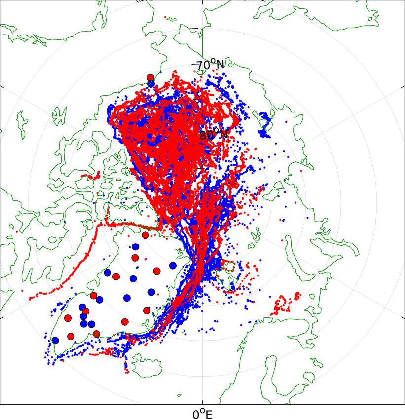
3036                                      P. Nielsen-Englyst et al.: Deriving Arctic 2 m air temperatures over snow and ice

et al., 2010; IPCC, 2013; Morice et al., 2012; Smith et al.,       cloud cover were identified as key parameters determining
2008; Vose et al., 2012). These datasets typically have higher     the T2m–ISTskin difference.
uncertainties in the Arctic region due to the limited availabil-      The second challenge, related to the use of satellite-
ity of in situ observations (Cowtan and Way, 2014; Lenssen         derived infrared ISTskin to derive T2m, is that the availabil-
et al., 2019; Rapaić et al., 2015). In addition, global reanal-   ity of ISTskin observations is limited to clear-sky conditions
ysis products such as ERA-Interim (ERA-I) and ERA5 (Dee            while T2m is measured continuously by AWSs and buoys.
et al., 2011; Hersbach et al., 2020) are frequently used to        Previous studies have shown that a satellite-derived, clear-
study the changes in the Arctic and to force ocean and sea ice     sky, surface temperature record can be significantly colder
models. Despite the assimilation of in situ data in the global     than an all-sky surface temperature record (Koenig and Hall,
reanalysis models, significant model differences have been         2010; Nielsen-Englyst et al., 2019). To benefit from the
reported for the Arctic (Davy and Outten, 2020; Delhasse et        good coverage of satellite surface temperature data, above-
al., 2020; Lindsay et al., 2014; Wesslén et al., 2014) as well     mentioned challenges should be considered with caution.
as large deviations from observations of T2m over Arctic sea       This work, starting with Nielsen-Englyst et al. (2019), has
ice (Wang et al., 2019).                                           been initiated to estimate clear-sky T2m from satellite ob-
   Observations from polar-orbiting satellites offer a very        servations (whenever these are available) for the Arctic sea
good supplement to the in situ observations through high spa-      ice and the GrIS in order to provide spatially detailed obser-
tial and temporal coverage of the high latitudes and may im-       vations for the areas unobserved by in situ stations and to
prove the surface temperature products and the assessment          supplement the in situ observations already available. Here,
of the Arctic climate changes. Therefore, daily near-surface       special attention has been given to the above-mentioned chal-
air temperatures derived from satellite temperature observa-       lenges, and the relationships between the near-surface air
tions have the potential to increase the amount of informa-        temperature and the satellite skin measurements have been
tion in the datasets and improve the quality of the climate        explored in detail. A regression-based approach has been
records, as recognized in Merchant et al. (2013) and Rayner        used to estimate daily T2m using satellite ISTskin and a sea-
et al. (2020).                                                     sonal cycle function as predictors based on the work pre-
   Two fundamental challenges exist when deriving a T2m            sented in Høyer et al. (2018). The derived product covers
product from infrared satellite observations. The first chal-      only days with no or limited clouds, when satellite skin tem-
lenge is that infrared sensors (in the atmospheric window          perature observations are available. However, for those days
region of 10–12 µm wavelength) measure the ice surface             when the satellite-derived T2m product is available, it pro-
skin temperature (ISTskin ), whereas the current global tem-       vides an estimate of the daily averaged all-sky T2m since it
perature products include the near-surface air temperature         has been regressed towards in situ measurements from both
as measured continuously by AWSs and buoys. The sur-               clear and cloudy conditions. In order to further facilitate the
face skin temperature may differ considerably from the near-       usage of the derived product in modelling and for monitoring
surface air temperature measured by AWSs or buoys. Pre-            purposes, each satellite-retrieved T2m estimate comes with
vious studies have compared satellite-retrieved ISTskin and        uncertainties.
T2m from AWSs located on the Greenland Ice Sheet (GrIS;               Similar efforts have been made to estimate clear-sky near-
Dybkjær et al., 2012a; Hall et al., 2008, 2012; Koenig and         surface air temperatures (and corresponding uncertainties)
Hall, 2010; Shuman et al., 2014) and over the Arctic sea           over land, ocean, and lakes using satellite observations to
ice (Dybkjær et al., 2012) and found temperature differences       cover all surfaces of the Earth (Good, 2015; Good et al.,
of which a significant part could be attributed to the tem-        2017; Høyer et al., 2018). The previous work has mostly been
perature difference between T2m and ISTskin . Other studies        done as a part of the European Union’s Horizon2020 project
have investigated the relationship between T2m and ISTskin         EUSTACE (EU Surface Temperatures for All Corners of
over ice using in situ observations (Adolph et al., 2018;          Earth, 2015–2019, https://www.eustaceproject.org, last ac-
Hall et al., 2008, 2004; Hudson and Brandt, 2005; Nielsen-         cess: 29 June 2021), with the overall aim to produce a glob-
Englyst et al., 2019; Vihma et al., 2008). Nielsen-Englyst         ally complete gap-free daily near-surface temperature analy-
et al. (2019) found that on average T2m is 0.65–2.65 ◦ C           sis since 1850. It is outside the scope of this paper to produce
higher than ISTskin with variations depending on the loca-         a daily continuous gap-free near-surface temperature analy-
tion of the measurement, i.e. over sea ice, seasonal snow          sis. However, within EUSTACE this has been done using a
cover, and the following zones of the GrIS: lower ablation         statistical model to combine satellite-derived clear-sky near-
zone, upper-middle ablation zone, and accumulation zone.           surface air temperatures and in situ observations and their
The T2m–ISTskin difference was found to vary seasonally            respective uncertainty estimates (Morice et al., 2019; Rayner
with the largest differences during the winter (when inver-        et al., 2020). The clear-sky T2m product derived in this pa-
sions are most common) and during melting conditions in the        per has been used to generate this daily gap-free EUSTACE
summer (where the surface temperature is fixed at the melt-        T2m product for the GrIS and the Arctic sea ice, while simi-
ing point). In Nielsen-Englyst et al. (2019), wind speed and       lar clear-sky temperature products have been used over land,
                                                                   ocean, and lakes.

The Cryosphere, 15, 3035–3057, 2021                                                   https://doi.org/10.5194/tc-15-3035-2021
P. Nielsen-Englyst et al.: Deriving Arctic 2 m air temperatures over snow and ice                                             3037

   This paper is structured such that Sect. 2 describes the in
situ data and the satellite data. Section 3 presents the method
used to estimate clear-sky daily T2m and uncertainties. The
resulting T2m dataset and its validation are presented in
Sect. 4 and discussed in Sect. 5. Conclusions are given in
Sect. 6.

2     Data

2.1    In situ data
                                                                  Figure 1. Total number of daily averaged in situ observations of
In situ observations of near-surface air temperatures have        T2m and ISTskin over Arctic land ice and sea ice per year covering
been collected from weather stations, expeditions, and cam-       the period 2000–2009.
paigns covering ice and snow surfaces to assemble the DMI-
EUSTACE database. The database includes quality con-
trolled and uniformly formatted temperature observations             The different in situ types measure the air temperature at
covering ice and snow surfaces during the period 2000–2009        different heights that furthermore differ over time depend-
(Høyer et al., 2018). For the GrIS we use the Programme           ing on the amount of snowfall, snow drift, and snowmelt.
for Monitoring of the Greenland Ice Sheet (PROMICE) data          Here, we will refer to T2m for all observation types regard-
provided by the Geological Survey of Denmark and Green-           less of these variations. Nielsen-Englyst et al. (2019) showed
land (GEUS; Fausto and van As, 2019; Ahlstrøm et al., 2008;       small changes (< 0.22 ◦ C) in T2m–ISTskin differences when
van As et al., 2011) and the Greenland Climate Network data       using only observations within the measurement range of
(GC-Net; Kindig, 2010; Shuman et al., 2001; Steffen and           1.90–2.10 m in height compared to using all measurements
Box, 2001). Only PROMICE data from the middle-upper ab-           (ranging in measurement height from 0.3 to 3 m). The obser-
lation zone and accumulation zone have been used to ensure        vations from Polarstern at 29 m height are not included in the
that data are only acquired over permanently snow- or ice-        derivation of the near-surface air temperature dataset but only
covered surfaces. Observations covering seasonal snow have        used for the validation. The accuracy of the air temperature
also been used from the Atmospheric Radiation Measure-            sensors for all observation sites is approximated to 0.1 ◦ C
ment (ARM) programme from two sites: Atqasuk (ATQ) and            (Hall et al., 2008; Høyer et al., 2017b). Few data sources
Barrow (BAR), at the North Slope of Alaska (Ackerman and          provide both skin and air temperatures, e.g. the PROMICE
Stokes, 2003; Stamnes et al., 1999). Data from Arctic sea ice     and ARM stations. The PROMICE skin temperatures have
are primarily retrieved from the meteorological observation       been calculated from upwelling longwave radiation, mea-
archive at the European Centre for Medium-Range Weather           sured by Kipp & Zonen CNR1 or CNR4 radiometers, assum-
Forecasts (ECMWF) MARS data storage facility, providing           ing a surface longwave emissivity of 0.97 (van As, 2011). All
196 unique data series from drifting buoys. These sea ice         in situ data have been screened for spikes and other unreal-
data are supplemented with data from 10 US Army Cold              istic data artefacts by visual inspection. Afterwards, the in
Regions Research Engineering Laboratory (CRREL) mass              situ observations have been averaged to daily temperatures
balance buoys (Perovich et al., 2016; Richter-Menge et al.,       using all available observations. Figure 1 shows the number
2006) and observations from a weather station located 29 m        of daily averaged in situ observations each year (2000–2009)
above the sea surface on the research vessel Polarstern op-       of ISTskin and T2m over Arctic land ice and sea ice. The two
erated by the Alfred Wegener Institute in the sea-ice-covered     ARM stations are included as land ice stations in this anal-
parts of the Arctic Ocean (Knust, 2017; König-Langlo et al.,      ysis, and only data from snow-covered periods are used. In
2006a). We also use air temperature measurements obtained         total 65 810 observations with daily T2m and 7057 observa-
from ice buoys deployed in the Fram Strait region within          tions with daily ISTskin are available over land ice. See Ta-
the framework of the Fram Strait Cyclones (FRAMZY) cam-           ble 1 for more information on the in situ observations used
paigns during the years 2002, 2007, and 2008 as well as air       in this study.
temperatures from the Arctic Climate System Study (AC-
SYS) campaign in 2003 (Brümmer et al., 2011b, c, 2012b, a).       2.2   Satellite data
Finally, we use data from two ice buoy campaigns operated
by the Meteorological Institute of the University of Hamburg      The satellite data used in this study are from the Arctic and
within the framework of the integrated EU research project        Antarctic Ice Surface Temperatures from thermal Infrared
DAMOCLES (Developing Arctic Modelling and Observing               satellite sensors (AASTI; Dybkjær et al., 2014, 2018; Høyer
Capabilities for Long-term Environmental Studies; Brümmer         et al., 2019) dataset, covering high-latitude seas, sea ice,
et al., 2011a).                                                   and ice sheet with clear-sky surface temperatures based on
                                                                  satellite infrared measurements from the CLARA-A1 dataset

https://doi.org/10.5194/tc-15-3035-2021                                                  The Cryosphere, 15, 3035–3057, 2021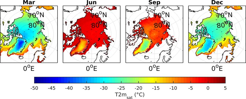
3038                                         P. Nielsen-Englyst et al.: Deriving Arctic 2 m air temperatures over snow and ice

Table 1. Overview of in situ observations used in this study, covering the period 2000–2009.

                           No. of sites,      No. of days        Surface type      Observation type    Temperature measurements
                           (AWS, buoys,       with observa-
                           or ships)          tions
        ACSYS                            7                280    Sea ice           Buoy                T2m
        ARM                              2              2846     Seasonal snow     AWS                 T2m, ISTskin
        CRREL                           10              1031     Sea ice           Buoy                T2m
        DAMOCLES                        25              2160     Sea ice           Buoy                T2m
        ECMWF                          196             27 235    Sea ice           Buoy                T2m
        FRAMZY                          11                251    Sea ice           Buoy                T2m
        GC-NET                          15             29 133    Land ice          AWS                 T2m
        POLARSTERN                       1                189    Sea ice           Ship                T2m
        PROMICE                          8              2685     Land ice          AWS                 T2m, ISTskin

compiled by EUMETSAT’s Climate Monitoring, Satellite                    the sea surface temperature (SST) community (Bulgin et al.,
Application Facility (CM-SAF; Karlsson et al., 2013). The               2016; Rayner et al., 2015) and will be followed here. The
dataset is based on one of the longest existing satellite               total uncertainty on the ISTskin_L2 , µtotal_L2 , is calculated by
records from the Advanced Very High Resolution Radiome-                 summing each component in quadrature (i.e. square root of
ter (AVHRR) instruments on board a long series of NOAA                  sum of squares). Excluding the cloud mask uncertainty, grid
satellites. AASTI contains swath-based (i.e. Level 2; L2) ice           cell systematic uncertainties (µglob_L2 ) are set to a fixed value
surface skin temperature (ISTskin_L2 ) data processed and er-           of 0.1 ◦ C to represent systematic uncertainties in the forward
ror corrected on the original Global Area Coverage (GAC)                models (see e.g. Merchant et al., 1999; Merchant and Le
grid. The first version of the AASTI product, which is used             Borgne, 2004). The AASTI ISTskin_L2 data also come with a
in this study, is available from 2000 to 2009 in the original           quality level (QL) from 1 (bad data) to 5 (best quality), with
projection and resolution (L2), i.e. ∼ 0.05 arc degree resolu-          the addition of level 0 (no data) (GHRSST Science Team,
tion and multiple daily coverage. Since 2000, seven different           2010).
AVHRR instruments have been orbiting the globe, each 14                    Here, we have aggregated the AASTI ISTskin_L2 observa-
times per day, thus providing approximately bi-hourly cover-            tions into 3-hourly and daily gridded Level 3 (L3) averages
age of the polar regions (Fig. 2). The number of operational            of ISTskin_L2 on a fixed 0.25◦ by 0.25◦ regular geographical
satellites increased from two to six from 2000 to 2009. The             grid. This grid was chosen within the EUSTACE project to
IST algorithm used to generate the AASTI dataset is based on            ensure a common grid to be used globally. The daily gridded
thermal infrared brightness temperatures of AVHRR chan-                 averages (ISTskin_L3 ) are calculated by averaging all avail-
nels 4 (centre wavelength at ∼ 11 µm) and 5 (centre wave-               able ISTskin_L2 observations with a quality flag of 4 (good)
length at ∼ 12 µm) and the satellite zenith angle. The al-              or 5 (best) for a given date and within the 0.25◦ bin. This
gorithm is a split window algorithm, working within three               has been done to facilitate the development of the relation-
temperature domains for each individual satellite (Key et al.,          ship model and to ease the user uptake. The data in the daily
1997). The retrieval calibration of each domain has been                aggregated files contain mean surface temperature observa-
done by relating modelled surface temperatures with mod-                tions from 00:00 to 24:00 LST, 3-hourly bin averages of sur-
elled top-of-atmosphere brightness temperatures, determined             face temperatures, and also the number of observations in
by a radiative transfer model (Dybkjær et al., 2014). Cloud             the eight time bins during each day. The 3-hourly numbers
masking has been performed using the Polar Platform Sys-                of observations are used to estimate the satellite sampling
tem (PPS) cloud processing software (Dybbroe et al., 2005a,             throughout the day, and the 3-hourly temperature data are
b).                                                                     used to gain confidence in the daily cycle estimates (see qual-
   As discussed in Merchant et al. (2017), satellite-based cli-         ity checks below). Figure 3 shows the mean number of ob-
mate data records should include uncertainty estimates. The             servations per day in each of the eight time intervals given
AASTI ISTskin_L2 data come with uncertainties divided into              in local time for the Arctic region. The variation in cover-
three independent uncertainty components, each with differ-             age throughout the day is a combined effect of the satellite
ent characteristics: the random uncertainty (µrnd_L2 ), a lo-           overpassing, performance of the cloud screening algorithm,
cally systematic uncertainty (µlocal_L2 ), and a large-scale sys-       and the cloud-free conditions during the day. In addition, the
tematic (“global”) uncertainty (µglob_L2 ). These three com-            fixed 0.25◦ regular geographical grid results in a decreasing
ponents have been chosen since they behave differently when             L3 bin area when approaching the North Pole. The maximum
aggregating the observations in time or space (see Sect. 3.2).          satellite coverage is generally seen around 80◦ N with a min-
This uncertainty methodology has been developed within

The Cryosphere, 15, 3035–3057, 2021                                                            https://doi.org/10.5194/tc-15-3035-2021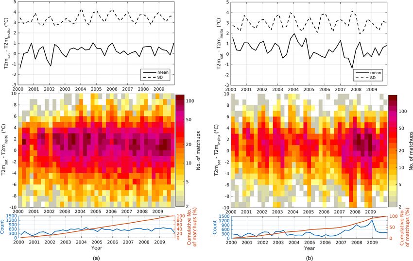
P. Nielsen-Englyst et al.: Deriving Arctic 2 m air temperatures over snow and ice                                             3039

Figure 2. NOAA and Metop satellites carrying the AVHRR sensor, used for AASTI version 1.

imum at the North Pole. Cloud-free conditions over the GrIS         ations during the summer in Greenland and during the win-
are primarily observed around noon and the early afternoon.         ter for sea ice, when the freeze-up of sea ice causes higher
   In order to best resolve the diurnal cycle with satellite        variability along the sea ice margin (Fig. 4). The main uncer-
information, we require data during both the night (be-             tainty components of the ISTskin_L3 estimates are erroneous
tween 18:00 and 06:00 LST) and the day (between 06:00 and           cloud screening and the spatial variance of snow and ice sur-
18:00 LST) in order to calculate ISTskin_L3 . To identify sea       face emissivity, which are not accounted for in the retrieval
ice, we use an ice mask for which sea ice is characterized by       algorithm. The presence of non-detected clouds will con-
sea ice concentrations above 30 % according to the EUMET-           tribute to increased standard deviations and usually a cold
SAT OSISAF Global Sea Ice Concentration Climate Data                ISTskin_L3 bias, since the cloud tops and other atmospheric
Record (Tonboe et al., 2016). A few more checks have been           constituents are generally colder than the surface (Dybkjær
set up in order to minimize the temporal sampling errors, the       et al., 2012).
effects of undetected clouds and outliers, and inconsistencies
between the ice mask and the surface temperatures. Follow-          2.2.1   Validation
ing Høyer et al. (2018), the ISTskin_L3 is discarded if one of
the following criteria is met:                                      Additional satellite versus in situ differences arise when
                                                                    comparing satellite observations with pointwise ground mea-
  – ISTskin_L3 exceeds +5 ◦ C, indicating inconsistency be-         surements due to different spatial and temporal characteris-
    tween the ice mask and the surface temperatures.                tics. To assess the magnitude of these effects, the ISTskin_L3
  – The standard deviation of satellite ISTskin_L2 during 1 d       data have been validated against in situ observations from the
    exceeds 7.07 ◦ C, corresponding to a sinusoidal daily cy-       PROMICE and ARM stations. Table 2 shows the validation
    cle with a difference between day and night of 20 ◦ C.          results of daily ISTskin_L3 against in situ skin temperatures
                                                                    (ISTskin_insitu ) and in situ 2 m air temperatures (T2minsitu ).
  – The difference between ISTskin_L3 and the average of all        The maximum matchup distance is 14.6 km, and the aver-
    available 3 h bin averages exceeds 10 ◦ C.                      age distance is 8.1 km, considering the AWSs in Table 2.
                                                                    The topography mask included in the HIRHAM5 regional
  – ISTskin_L3 is more than 10 ◦ C colder than the corre-
                                                                    climate model (see e.g. Langen et al., 2015) has been used
    sponding average of up to 24 neighbouring cloud-free
                                                                    to calculate the differences in elevation (1h) between the
    observations (in a 5-by-5 grid cell square) with the same
                                                                    in situ stations and corresponding satellite pixels. There is
    surface type.
                                                                    no clear correlation between the large biases and large ele-
The criteria above have been derived from analysis and in-          vation differences from this table, but the elevation effects
spection of the satellite data and with considerations to the       are contributing to the spatial sampling error. The spatial
results presented in Nielsen-Englyst et al. (2019). Inconsis-       and temporal sampling errors contribute to the overall un-
tencies between the ice mask and surface temperature typi-          certainty, but effects from erroneous cloud screening, algo-
cally occur along the coasts and sea ice edge, where the OS-        rithm simplifications, and uncertainties in the in situ ob-
ISAF product is subject to land-spillover effects causing spu-      servations are also included in the results. Previous stud-
rious ice in ice-free areas (Lavergne et al., 2019). Using a sur-   ies find that erroneous cloud screening (undetected clouds)
face temperature threshold of 5 ◦ C reduces the land-spillover      is one of the main reasons for the cold biases observed
effects and results in increased consistency between the ice        when comparing satellite-observed IST with in situ mea-
mask and the surface temperatures.                                  surements (Hall et al., 2004, 2012; Koenig and Hall, 2010;
   The satellite-derived surface temperature has seasonal dif-      Østby et al., 2014; Westermann et al., 2012). Another impor-
ferences in daily variability, with the largest standard devi-      tant contribution is the effect of comparing clear-sky satel-

https://doi.org/10.5194/tc-15-3035-2021                                                    The Cryosphere, 15, 3035–3057, 2021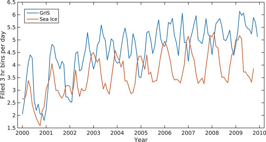
3040                                       P. Nielsen-Englyst et al.: Deriving Arctic 2 m air temperatures over snow and ice

Figure 3. Mean number of observations per day in the L3 bins for each of the eight local solar time intervals, averaged for the period
2000–2009.

Figure 4. Standard deviations (◦ C) of daily satellite surface temperature observations for March, June, September, and December of each
year averaged for the years 2000–2009.

lite observations with all-sky in situ observations, as dis-          tic (2–5 d) and seasonal variations, which are pronounced in
cussed in Nielsen-Englyst et al. (2019). In general, ISTskin_L3       both IST and T2m.
correlates better with T2minsitu than with the ISTskin_insitu .
Moreover, the ISTskin_L3 –T2mInSitu difference shows smaller
standard deviations than ISTskin_L3 –ISTskin_insitu . However,        3     Methods
as expected the biases and root-mean-squared differences
                                                                      3.1    Regression model
(RMSDs) are larger for the ISTskin_L3 –T2minsitu differences
than for the ISTskin_L3 –ISTskin_insitu differences. The reason       Nielsen-Englyst et al. (2019) analysed a large number of in
is that the radiometric surface skin temperature can be sig-          situ stations with simultaneous T2m and ISTskin observations
nificantly different from the surface air temperature mea-            and showed that empirical relationships exist between T2m
surements (Adolph et al., 2018; Hall et al., 2008; Hudson             and ISTskin . However, it was also shown that the relationships
and Brandt, 2005; Nielsen-Englyst et al., 2019; Vihma et al.,         varied for different regions. Based upon these results, it was
2008). On average, the skin temperature is colder than the            decided to use a simple-regression-based method in this pa-
air temperature (Nielsen-Englyst et al., 2019), resulting in          per to derive the daily mean T2m from the satellite ISTskin_L3
even more negative biases, when the ISTskin_L3 is compared            observations. Separate regression models have been derived
to in situ measured T2m, instead of in situ skin temperatures.        for land ice and sea ice.
The generally high correlations are dominated by the synop-

The Cryosphere, 15, 3035–3057, 2021                                                        https://doi.org/10.5194/tc-15-3035-2021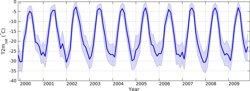
P. Nielsen-Englyst et al.: Deriving Arctic 2 m air temperatures over snow and ice 3041
Table 2. Validation of daily AASTI v.1 Level 3 IST (ISTskin_L3 ) against in situ ISTskin (ISTskin_insitu ) and T2m observations (T2minsitu ).
N: number of matchups; Corr: correlation; SD: standard deviation; RMSD: root-mean-square difference. d is the matchup distance and 1h
is the difference in elevation (AWS − satellite).
ISTskin_L3 − ISTskin_insitu ISTskin_L3 − T2minsitu d (km) 1h (m)
Station N Corr Bias SD RMSD Corr Bias SD RMSD
ARM_ATQ 1235 93.8 −2.47 3.69 4.44 93.7 −3.17 3.69 4.87 10.8 –
ARM_BAR 1594 94.1 −0.73 4.30 4.36 94.6 −1.14 4.02 3.86 6.1 –
PROMICE KAN-M 422 93.9 −3.65 3.37 4.96 94.6 −4.56 3.14 5.53 7.6 15
PROMICE KAN-U 239 93.9 −1.75 3.32 3.75 94.4 −3.39 3.17 4.64 14.6 21
PROMICE KPC-U 488 97.6 −1.31 2.62 2.92 98.2 −3.20 2.27 3.92 5.1 29
PROMICE NUK-U 296 77.7 −4.09 5.00 6.45 84.7 −7.19 4.01 8.23 14.4 64
PROMICE QAS-U 407 83.9 −1.65 4.20 4.51 86.3 −3.70 3.75 5.27 6.5 197
PROMICE SCO-U 403 91.5 −4.60 4.25 6.26 93.7 −7.55 3.75 8.43 4.2 20
PROMICE TAS-U 386 67.5 −1.03 5.43 5.52 79.5 −3.61 4.39 5.68 8.4 214
PROMICE UPE-U 125 88.2 −3.13 3.88 4.97 90.0 −5.49 3.50 6.50 3.0 110
All data 5595 92.9 −2.03 4.24 4.70 93.2 −3.36 4.12 5.32 8.1 83.8
To test different types of regression models, the ISTskin_L3
data have been matched up with in situ observations for each
day (Høyer et al., 2018). This is done by requiring a dis-
tance to the nearest in situ site of less than 15 km. The aver-
age matchup distance is 8.6 and 7.2 km for land ice and sea
ice, respectively, which means that all in situ observations are
made within the area of the satellite pixel. The corresponding
mean elevation difference is 30 m (while the absolute mean
elevation difference is 45 m) and is calculated using the to-
pography mask included in HIRHAM5 (Langen et al., 2015)
for the 23 GrIS AWSs. Out of the 23 AWSs, four of them
(GC-net JAR1, TAS_U, QAS_U, and UPE_U) have corre-
sponding elevation differences above 100 m. In Sect. 4.3,
the effect of these AWSs has been estimated and discussed.
All in situ observations, described in Sect. 2.1., have been
matched with ISTskin_L3 data, resulting in a total number of
daily matchups of 65 810 from 275 different observation sites
(see Table 1). These have been divided into two subsets: one
for training and one for validation of the different regression
models for land ice and sea ice, respectively. This has been
done while ensuring similar coverage of training and vali-
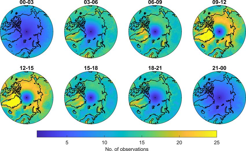
dation data over the two domains, which is shown in Fig. 5. Figure 5. Positions of matchups on sea ice and land ice (red: train-
The result is that 40 % (13 792 matchups) are used for testing ing; blue: validation).
the regression models (and generating the regression coeffi-
cients), and the remaining 60 % (20 872 matchups) are left
for validation of the regression models over land ice. Over where d obs and d pre are vectors containing the observed and
sea ice 48 % (15 035 matchups) are used for testing, and 52 % modelled in situ air temperatures, respectively, G is a matrix
(16 111 matchups) are left for validation. containing the various predictors, m is a vector containing
The regression model is based on multiple linear regres- regression coefficients, and e is the fitting error.
sion analysis using least squares (Menke, 1989). The mul- The regression coefficients are found using damped least
tiple linear regression analysis equations can be written in squares (Menke, 1989). The least-squares method is used
matrix form, since the problem is generally over-determined, and the
damping is added to limit effects of noisy data. The regres-
d obs = Gm + e, (1) sion coefficients are thus given as
pre
d = Gm, (2)
https://doi.org/10.5194/tc-15-3035-2021 The Cryosphere, 15, 3035–3057, 2021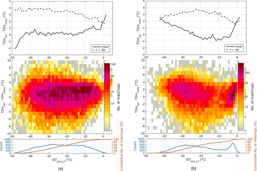
3042                                         P. Nielsen-Englyst et al.: Deriving Arctic 2 m air temperatures over snow and ice

                                                                      Table 3. Statistics on the relation between observed and modelled
                    −1                                              temperatures for the training data. N: number of matchups used
G−g = GT G + ε 2 I         GT ,                                 (3)   for testing; Corr: correlation; RMSD: root-mean-square difference.
                                                                      Since, the training data are used for the regression, the bias is zero,
m = G−g d obs ,                                                 (4)   and thus the standard deviation equals RMSD.

where G−g is called the generalized inverse, ε is a damping                                                 N     Corr (%)    RMSD (◦ C)
factor, and I is an identity matrix (with ones in the diago-
                                                                       Land ice    ÎSTskin              13 792        95.7            3.51
nal and zeros elsewhere). The superscript operator T denotes                       ÎSTskin SWd          13 792        96.2            3.28
transposing and −1 denotes inversion. We have tested a range                       ÎSTskin WSERA-I      13 792        95.8            3.47
of damping factors to assess the relation to the error coeffi-                     ÎSTskin WSERA5       13 792        95.9            3.42
cients. A damping factor of 0.2 was chosen to avoid over-                          ÎSTskin Lat          13 792        95.8            3.48
fitting noise in the data, while keeping the error coefficients                    ÎSTskin Season       13 792        96.3            3.28
low.                                                                   Sea ice     ÎSTskin              15 035        96.0            3.32
    The choice of predictors is based on current knowledge                         ÎSTskin SWd          15 035        96.0            3.32
of the parameters that influence the relationship between                          ÎSTskin WSERA-I      15 035        96.0            3.32
ISTskin and T2minsitu (Adolph et al., 2018; Hall et al., 2008;                     ÎSTskin WSERA5       15 035        96.0            3.32
Hudson and Brandt, 2005; Nielsen-Englyst et al., 2019;                             ÎSTskin Lat          15 035        96.1            3.28
Vihma and Pirazzini, 2005), limited by the available satel-                        ÎSTskin Season       15 035        96.2            3.25
lite data. Nielsen-Englyst et al. (2019) showed that the T2m–
Tskin difference varies over the season with the smallest
differences during the spring, autumn, and summer in non-             sin(x1 ) sin(x2 ), the seasonal
                                                                                                  q cycle can be rewritten to the
melting conditions. For that reason, we have also tested the
                                                                      form in Eq. (12) with A = α22 + α32 and ϕ = arctan(α3 /α2 ).
effect of including a seasonal cycle as predictor. A total of
five regression models with different predictors have been               The training data have been used to calculate the re-
tested (Høyer et al., 2018).                                          gression coefficients for each regression model covering the
                                                                      land ice and sea ice. The performance of each regression
ÎSTskin :           T2msat = α0 + α1 ISTskin_L3                 (5)   model has been investigated using the training data, and
                                                                      the results are shown in Table 3. The best performance is
ÎSTskin SWd :       T2msat = α0 + α1 ISTskin_L3                       found by using the regression model where T2msat is pre-
                                  + α2 SWd                      (6)   dicted from ISTskin_L3 combined with a seasonal variation
ÎSTskin WS :        T2msat = α0 + α1 ISTskin_L3                       (ÎSTskin Season). This model predicts T2msat better compared
                                                                      to the other regression models, with correlations above 96 %
                                  + α2 WS                       (7)
                                                                      and RMSD values of 3.25–3.28 ◦ C against training data for
ÎSTskin Lat :       T2msat = α0 + α1 ISTskin_L3                       both surface types (Table 3). In the following, we will use the
                                  + α2 Lat                      (8)   regression model given in Eq. (12) with the seasonal term in-
                                                                      cluded and with separate regression coefficients for land ice
ÎSTskin Season :    T2msat = α0 + α1 ISTskin_L3
                                                                      and sea ice (see Table 4). The phase corresponds to a maxi-
                                  + α2 cos ((t · 2π )/(1 yr))         mum on the 19 January and 12 February for land ice and sea
                                  + α3 sin ((t · 2π )/(1 yr))   (9)   ice, respectively. This is in agreement with Nielsen-Englyst
                                                                      et al. (2019), who found the strongest clear-sky inversion dur-
The regression model in Eq. (8) is limited to an offset and           ing the winter months (December–February) for all sites in-
a scaling of ISTskin_L3 , where the latter term accounts for          cluded in the analysis except from the ones located in the
the synoptic and seasonal variations, which are the dominat-          lower ablation zone (not included here), where pronounced
ing factors in both the IST and T2m variability. This part            surface melt takes place for long periods of time.
is thus included in all regression models tested. The other
regression models also have a third predictor, which is in-           3.2   Uncertainty estimates for T2msat
cluded to examine how to best represent the residual varia-
tions in the T2m–IST difference. The model in Eq. (9) uses            Uncertainty estimates on the derived T2msat are crucial
theoretical top-of-atmosphere shortwave radiation, Eq. (10)           to facilitate the usage of the dataset in modelling and
uses the wind forcing (from ERA-I and ERA5, respectively),            for monitoring purposes. The uncertainty estimates of the
Eq. (11) uses latitude variation, and Eq. (12) uses a seasonal        satellite-derived T2msat data follow the approach in Bulgin
variation. In the regression model in Eq. (12), the seasonal          et al. (2016) and Rayner et al. (2015), which has also been
variation is assumed to be the shape of a cosine function,            used for the AASTI data. The uncertainty on a single T2msat
A·cos((t ·2π )/(1 yr)−ϕ), where A is the amplitude, ϕ is the          estimate is divided into random, locally correlated, and sys-
phase and t is time. Since cos(x1 − x2 ) = cos(x1 ) cos(x2 ) +        tematic uncertainty components, with the total uncertainty

The Cryosphere, 15, 3035–3057, 2021                                                         https://doi.org/10.5194/tc-15-3035-2021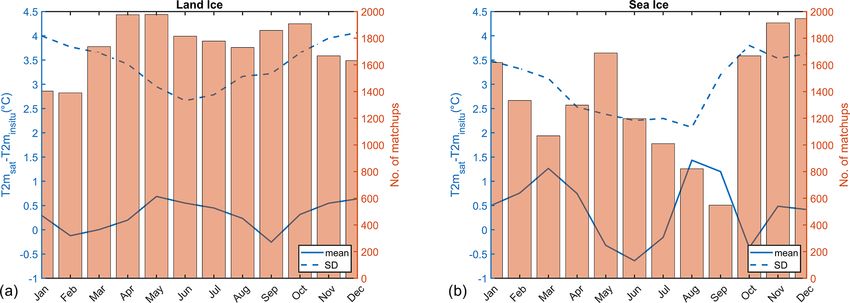
P. Nielsen-Englyst et al.: Deriving Arctic 2 m air temperatures over snow and ice                                                  3043

Table 4. Model regression coefficients for ÎSTskin Season.

                                         Offset, α0 (◦ C)    ISTskin_L3 factor, α1   Amplitude, A    Phase, ϕ
                             Land ice               4.20                     1.06            2.26      −0.33
                             Sea ice                1.46                     0.89            1.83      −0.75

µtotal_T2m given as the square root of the sum of the three              very challenging task and is out of the scope of this paper.
squared components:                                                      Instead, we estimate the µlocal_T2m component using a sim-
             q                                                           ple regression model fitted to the satellite-derived T2m and
µtotal_T2m = µ2rnd_T2m + µ2local_T2m + µ2glob_T2m .                      in situ T2m differences. Separate models have been chosen
                                                                         for the land ice and sea ice, due to the differences in the er-
The random uncertainty component for the T2msat belong-                  ror characteristics. The variables to include in the uncertainty
ing to a particular grid cell at a particular point in time is           regression models have been chosen from a careful examina-
found by propagating the AASTI ISTskin_L3 random uncer-                  tion of the matchup dataset. For land ice and sea ice the most
tainty through the regression model:                                     relevant variables were the ISTskin_L3 itself and the number
            q                                                            of 3 h time bins with observations in the L3, Nbins .
µrnd_T2m = α1 µrnd_L3 ,
                          2                                                For land ice the regression model for µlocal_T2m is given as
                                                                         follows:
with µrnd_L3 given as the aggregated µrnd_L2 :                           µlocal_T2m_landice = β0 + β1 ISTskin_L3 + β2 Nbins ,       (10)
         µrnd_L2
µrnd_L3 = √      ,                                                       while the regression model for sea ice is given as
            N
                                                                         µlocal_T2m_seaice = γ0 + γ1 ISTskin_L3 + γ2 IST2skinL3
where N is the number of observations
                                   √       for each bin in the
aggregation from L2 to L3. The N reduction applies be-                                       + γ3 Nbins .                           (11)
cause the random uncertainty of each L2 data point that goes             The coefficients have been determined by fitting to the
into the L3 calculation is by definition independent from the            T2msat –T2minsitu standard deviations calculated for the train-
other.                                                                   ing data with ISTskin_L3 bin intervals of 2 ◦ C and a Nbins in-
   The L3 global uncertainty component does not average                  terval of 1. The µrnd_T2m and µglob_T2m components have
out in any aggregation and is thus transferred directly from             been removed from the standard deviations in each bin as
the L2 uncertainty estimate and multiplied by α1 to make up              well as an assumed in situ uncertainty of 0.1 ◦ C and an av-
µglob_T2m :                                                              erage sampling uncertainty of 0.5 ◦ C (Høyer et al., 2017a;
                                                                         Reeves Eyre and Zeng, 2017) before fitting the regression
µglob_T2m = α1 µglob_L3 = α1 · 0.1 ◦ C.                                  models. The optimal regression coefficients for each domain
                                                                         are listed in Table 5.
The µlocal_T2m contains the local uncertainty component of
L2, a sampling error µlsamp_L3 related to sampling errors
in space and time due to the aggregation, a relationship er-             4   Results
ror, cloud mask uncertainty, etc. When aggregating from L2
to daily L3, additional sources of uncertainty enter through             In Sect. 3.1, we selected the best (Eq. 12) of the five differ-
the gridding process as ISTskin_L3 can only be retrieved for             ent algorithms and used it together with the derived coeffi-
clear-sky pixels. This introduces a temporal and spatial sam-            cients (Tables 3 and 4) to retrieve T2m from satellite surface
pling uncertainty. If all our satellite observations were ob-            temperature estimates. The derived dataset consists of daily
tained during all-sky conditions, we assume that the high po-            estimates of near-surface air temperature on a 0.25◦ regular
lar temporal coverage is such that the temporal sampling un-             latitude–longitude grid, during the period 2000–2009 (Høyer
certainty in the L3 files can be set to zero. However, this is           et al., 2018; Kennedy et al., 2019). Days with clouds and
not the case, and using only clear-sky observations generally            few clear-sky observations (as explained in Sect. 2.2) are
leads to a clear-sky bias in averaged ISTskin satellite obser-           not included in the dataset. However, for those days when
vations when compared to in situ observations (Hall et al.,              the satellite-derived T2m product is available, it provides an
2012; Nielsen-Englyst et al., 2019; Rasmussen et al., 2018).             estimate of the daily averaged all-sky T2m (see Sect. 5).
The relationship error represents the standard deviation of the          Each temperature estimate is associated with three compo-
residuals calculated at in situ stations, where both skin and air        nents of uncertainty on the 0.25◦ daily scale: a random un-
temperatures are available, i.e. T2msat –T2minsitu . Estimating          certainty, a synoptic-scale correlated uncertainty, and a glob-
all the different components that make up the µlocal_T2m is a            ally correlated uncertainty excluding uncertainties related to

https://doi.org/10.5194/tc-15-3035-2021                                                        The Cryosphere, 15, 3035–3057, 2021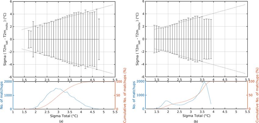
3044                                        P. Nielsen-Englyst et al.: Deriving Arctic 2 m air temperatures over snow and ice

Table 5. Uncertainty model regression coefficients.

                                 Land ice    β0 = 3.82 ◦ C   β1 = −0.24   β2 = −0.03
                                 Sea ice     γ0 = 2.01 ◦ C   γ1 = −0.06   γ2 = −0.12     γ3 = −0.001

the masking of clouds. The three types of uncertainties are
also gathered in a total uncertainty estimate (see Sect. 3.2).
The land ice temperatures have been calculated for grid cells
categorized as ice sheet by the ETOPO1 global relief model
(Amante and Eakins, 2009), averaged to the 0.25◦ grid. Sea
ice temperatures have been calculated for grid cells with sea
ice concentrations above 30 %, according to OSISAF (Ton-
boe et al., 2016).

4.1    Validation of T2msat

The derived T2msat product has been validated against in-
dependent in situ data (i.e. the validation subset described
in Sect. 3.1). Figure 6 shows an example of the daily near-
surface air temperature coverage (from 1 January 2008).
Circles are in situ T2m measurements from coincidence-
independent AWSs and buoys, and there seems to be quite
good agreement between these and T2msat during this spe-
cific day. The overall model performance, when compared to
                                                                     Figure 6. Daily mean 2 m air temperature over land ice and sea ice
all independent AWS and buoy observations, is summarized
                                                                     from 1 January 2008. Circles show in situ measurements.
in Table 6. The satellite-derived air temperatures are about
0.3 ◦ C warmer than measured in situ air temperature for both
land ice and sea ice. For the GrIS, the bias is partly explained
by topographic effects (see Sect. 4.3). The correlations are
above 95 % for both surface types, and the RMSD is 3.47              ture is expected over time. Figure 9 shows the average num-
and 3.20 ◦ C for land and sea ice, respectively. Note that the       ber of filled 3 h bins per day for the GrIS and Arctic sea ice
uncertainty of the in situ data is also included in these RMSD       for 2000–2009. Both surface types show an increase in filled
values.                                                              3 h bins over time, with large seasonal variations. In most
    Figure 7 shows the average seasonal variation in bias and        years, sea ice has 1–1.5 filled bins per day more during win-
standard deviation for land ice and sea ice, respectively. For       ter than summer, due to a more extensive cloud cover over sea
both land ice and sea ice, there is a seasonal dependency in         ice during summer (Curry et al., 1996; Beesley and Moritz,
standard deviation, with the largest values during the win-          1999). The GrIS typically has fewer filled bins per day dur-
ter and smallest values during the summer. This is likely ex-        ing the winter and summer than spring and autumn, which is
plained by a better cloud screening performance during sun-          also explained by differences in cloud coverage (Griggs and
lit periods (Karlsson and Dybbroe, 2010) and by the smaller          Bamber, 2008). Note that the increase in the average number
natural thermal variability that is observed during summer           of filled 3 h bins from 2000 to 2009 is not reflected in the
conditions. Similar seasonality in performance is seen in five       performance of the T2m product (Fig. 8).
reanalysis products (including ERA-I/ERA5) for the GrIS                 Figure 10 shows T2msat –T2minsitu differences plotted as a
(Zhang et al., 2021). As shown in Fig. 7, the average seasonal       function of AASTI L3 skin temperature for land ice and sea
variation in bias is largest over sea ice, with the largest val-     ice. Over land ice, the standard deviation decreases as a func-
ues in March and August. However, this seasonal tendency in          tion of ISTskin_L3 , while the bias is around zero for ISTskin_L3
bias over sea ice is only reflected at the beginning of the time     between −45 and −10 ◦ C, positive for higher temperatures
period (i.e. 2000–2004). This can be seen in Fig. 8, which           and negative for lower temperatures. For sea ice, the max-
shows the seasonal averaged independent validation statis-           imum standard deviation is found at skin temperatures of
tics for the entire period for land ice and sea ice. The figure      about −20 ◦ C, with smaller standard deviations for higher
also shows a quite stable performance over the time period           and lower ISTskin_L3 . Positive biases are found for very cold
for both land ice and sea ice.                                       skin temperatures (< −25 ◦ C) and for temperatures around
    As more satellite observations have become available over        the melting point (> −4 ◦ C), while the intermediate temper-
the time period, increased coverage of the surface tempera-          atures have a slightly negative bias. This effect is included

The Cryosphere, 15, 3035–3057, 2021                                                      https://doi.org/10.5194/tc-15-3035-2021
P. Nielsen-Englyst et al.: Deriving Arctic 2 m air temperatures over snow and ice 3045
Table 6. Statistics on the relation between satellite-derived and in situ measured temperatures for comparison with independent validation
data. N : number of matchups used for validation; Corr: correlation; bias: T2msat –T2minsitu difference; SD: standard deviation; RMSD:
root-mean-square difference.
N Corr (%) Bias (◦ C) SD (◦ C) RMSD (◦ C)
Land ice 20 872 95.5 0.30 3.45 3.47
Sea ice 16 111 96.5 0.35 3.18 3.20
Figure 7. Estimated T2m minus observed T2m averaged for each month for (a) land ice and (b) sea ice. The dashed lines are standard
deviations while the solid lines are biases. The bars show the average number of matchups for each month.
in the uncertainty estimates as presented in Sect. 3.2, which than for both T2mERA-I and T2mERA-5 , while the other vali-
include ISTskin_L3 as a predictor for both land ice and sea ice. dation parameters are similar, with slightly better correlation
Figure 11 shows the validation results of the estimated and standard deviation but slightly worse RMSD results for
uncertainties, where the T2msat –T2minsitu difference is plot- T2mERA . Previous studies have also found that ERA-I suf-
ted against the theoretical total uncertainties as obtained in fers from a consistent warm bias in the Arctic (Lüpkes et
Sect. 3.2 for land ice and sea ice. The dashed lines repre- al., 2010; Jakobson et al., 2012; Vihma et al., 2002; Batrak
sent the ideal uncertainty with the assumptions that the in and Müller, 2019; Simmons and Poli, 2014), and recent stud-
situ observations have an uncertainty of 0.1 ◦ C and that the ies suggest that the warm bias still exists in ERA5 over sea
sampling uncertainty is 0.5 ◦ C. The estimated uncertainties ice (Wang et al., 2019; Graham et al., 2019). Similarly, re-
show good agreement with the observed uncertainties when cent studies found no significant improvements in 2 m tem-
the error bars follow the dashed line, which is the case here peratures over the GrIS for ERA5 compared to ERA-I (Del-
for both land ice and sea ice. hasse et al., 2020; Zhang et al., 2021). Note, however, that the
NCEP-CFSR, which is based on a coupled atmosphere–sea
4.2 Comparison with reanalyses ice–ocean model, has shown better performance than ERA-I
for near-surface atmospheric variables over sea ice (Jakobson
The performance of T2msat has been compared to the perfor- et al., 2012).
mance of T2m from ECMWF’s reanalysis ERA-I (T2mERA-I ; Figure 12 shows the RMSD between in situ measured T2m
Dee et al., 2011) and the replacement reanalysis ERA5 and T2mERA-I as well as T2mERA5 and T2msat for the in-
(T2mERA5 ; Hersbach et al., 2020). Table 7 shows the perfor- dividual validation sites and both surface types. Due to the
mance of T2mERA-I and T2mERA5 against the independent in large number of buoys, these have been validated for each
situ T2m observations, which should be compared with the data source with all observations weighted equally. The last
performance of the regression-derived T2msat as shown in bars refer to the RMSD obtained by validating all valida-
Table 6. The comparison may not be truly independent as a tion sites in one long time series weighting all daily obser-
number of stations and buoys have been assimilated into the vations equally. The total T2msat agrees better with in situ
ERA-I and ERA5 data products (Dee et al., 2011; Hersbach observations for both surface types compared to both ERA-
et al., 2020), which would favour the reanalysis products in I and ERA5. For most land ice stations, the T2msat outper-
the comparison. Yet, the bias is significantly lower for T2msat
https://doi.org/10.5194/tc-15-3035-2021 The Cryosphere, 15, 3035–3057, 20213046 P. Nielsen-Englyst et al.: Deriving Arctic 2 m air temperatures over snow and ice
Figure 8. Estimated T2m minus observed T2m (bin size of 1 ◦ C) for the full time period (bin size of 90 d) for (a) land ice and (b) sea ice.
The dashed lines are standard deviations while the solid lines are bias in the upper figures. The surface plots in the middle figures show the
number of matchups in each bin, while the bottom plots show the number of matchups (blue) and the cumulative percentage of matchups
(red) in each time bin.
Table 7. Statistics on the relation between ERA-I/ERA5 and in situ measured temperatures for independent test data. N: number of matchups
used for validation; Corr: correlation; bias: T2mERA –T2minsitu difference; SD: standard deviation; RMSD: root-mean-square difference.
N Corr (%) Bias (◦ C) SD (◦ C) RMSD (◦ C)
Land ice 20 872 ERA-I 96.4 3.41 3.18 4.66
ERA5 97.1 2.03 3.08 3.69
Sea ice 16 111 ERA-I 96.9 1.14 3.02 3.22
ERA5 95.7 2.19 3.67 4.27
forms ERA-I and ERA5. One exception is the ARM sta- 29 m height. This is likely because the data are mainly from
tion (BAR), where a bias of 2.49 ◦ C gives rise to a relatively the summer, when the vertical temperature gradients in the
large RMSD for T2msat . This is likely explained by physi- boundary layer are mostly small, and the performance of the
cal differences between the seasonal snow-covered sites and cloud screening algorithm reaches its maximum. The inde-
the GrIS sites, which are not fully captured by the regres- pendent in situ observations by ACSYS, CRREL, DAMO-
sion model. ERA5 is significantly better than ERA-I over the CLES, and FRAMZY are better reproduced by the satellite-
GrIS, but ERA5 performs worse than both ERA-I and T2msat derived T2m. The errors in the T2mERA-I /T2mERA5 and
over sea ice. Over sea ice, T2mERA-I agrees better with in T2msat datasets are expected to be independent and uncor-
situ observations from the ECMWF data stream and Po- related. For that reason, a combination of either T2mERA-I or
larstern. However, these may be assimilated into both ERA- T2mERA5 and T2msat can lead to an improved T2m estimate.
I and ERA5. The validation against Polarstern is relatively
good even though the temperature measurements are made at
The Cryosphere, 15, 3035–3057, 2021 https://doi.org/10.5194/tc-15-3035-2021P. Nielsen-Englyst et al.: Deriving Arctic 2 m air temperatures over snow and ice 3047
variability is largest during winter due to a larger cloud ra-
diative effect (compared to near-zero during summer) and a
larger meridional temperature gradient resulting in a more
vigorous atmospheric circulation in winter (Serreze et al.,
1993). In addition, the temporal variability is lower during
summer due to the fact that when the surface begins to melt,
the sensible heat is used for melting and hence reducing sur-
face air temperature variability (Steffen, 1995).
As illustrated in Fig. 15, T2msat provides increasing cov-
erage over the period 2000–2003 and quite stable coverage
for the years 2003–2009. The average daily coverage is 84 %
and 67 % for land ice and sea ice, respectively, for the stable
Figure 9. Average number of filled 3 h bins per day for the Green- 2003–2009 period and the 0.25◦ grid. When considering a
land Ice Sheet and the Arctic sea ice. 1◦ grid resolution, these numbers increase to 94 % and 81 %,
respectively. Over land ice, the maximum coverage is during
the spring and autumn, while the sea ice coverage has a clear
4.3 Topographic effects
drop in coverage during the summer due to increased cloud
The effects from topography over the GrIS have been as- cover (Curry et al., 1996; Beesley and Moritz, 1999).
sessed by introducing a new matchup dataset that ensures that
the elevation difference between satellite and in situ observa-
tions is less than 100 m over the GrIS. Excluding those AWSs 5 Discussion
(4 out of 23) with a larger elevation difference than 100 m re-
sults in a reduction of the training dataset of 2935 matchups Due to the limited number of in situ observations in the Arc-
(i.e. from GC-net_JAR1 and PROMICE TAS_U) and a re- tic, and especially over sea ice, gathering in situ observations
duction in the validation dataset of 560 matchups (i.e. from for testing and validating the regression models is not a sim-
PROMICE QAS_U and UPE_U). The performance of the ple task. The lack of observations that represent all condi-
satellite-derived T2m improves the bias in particular, which tions and regions in the Arctic and the resulting matching
decreases to 0.07 ◦ C, while the standard deviation decreases threshold of 15 km combined with the large topographical
to 3.41 ◦ C over land ice. ERA-I and ERA5 show limited variations over the GrIS increase the uncertainty in the pixel-
changes in performance, with slightly increased biases of to-point comparison, thereby complicating the derivation and
3.48 and 2.07 ◦ C and standard deviations of 3.14 and 3.08 ◦ C, validation of the regression models. Despite this, the valida-
respectively, when introducing the new matchup dataset over tion against independent in situ observations and the com-
land ice. A similar good performance of the regression model parison with ERA-I and ERA5 demonstrate the value of the
is found when the two AWSs in the validation subset are kept. T2msat product in the Arctic.
Despite the increased performance of the regression model, Five regression models were tested, and the best regres-
we have included all observations in the training of the model sion model predicts T2msat from daily satellite ISTskin_L3
to ensure a robust and spatial representative solution. combined with a seasonal variation. The performance of the
T2msat product did not improve much when the wind speed
4.4 Analysis of T2msat information from ERA-I or ERA5 (Table 3) was included
despite the fact that previous studies have shown a strong
The monthly mean T2msat is shown in Fig. 13 for March, dependency of wind speed for both land ice and sea ice
June, September and December averaged over the period (Adolph et al., 2018; Hudson and Brandt, 2005; Miller et al.,
2000–2009. The interior and northern part of the GrIS is typi- 2013; Nielsen-Englyst et al., 2019). This was unexpected,
cally colder than other parts of the Arctic in all months, while at least for sea ice. The reason is likely that the quality of
the warmest regions are found along the sea ice marginal ice the wind speed fields is not adequate for use in the rela-
zone and the ablation zone of the GrIS. Limited spatial vari- tionship model. In particular, accurately representing kata-
ability is seen over the Arctic sea ice during summer. batic winds in numerical weather prediction (NWP) mod-
Figure 14 shows the monthly mean near-surface air tem- els is a challenging task due to the high resolution needed
perature estimates averaged over the GrIS for the period in the vertical direction (Grisogono et al., 2007; Steeneveld,
2000–2009. The GrIS records a distinct annual cycle in near- 2014; Weng and Taylor, 2003; Zilitinkevich et al., 2006).
surface air temperature, with the maximum temperatures of Furthermore, the representation of surface roughness and the
around −4 ◦ C during July and minimum temperatures of processes of snow–surface coupling, radiation, and turbulent
about −28 ◦ C during winter. The range in monthly mean air mixing are hampered by limited resolution, while the relative
temperature is in agreement with those reported by van As importance of the processes varies with wind speed (Sterk
et al. (2011) at a number of PROMICE AWSs. The temporal et al., 2013). More accurate information on the wind speed
https://doi.org/10.5194/tc-15-3035-2021 The Cryosphere, 15, 3035–3057, 2021You can also read