Design parameters analysis and verification of angular vibration sensor based on magnetohydrodynamics
←
→
Page content transcription
If your browser does not render page correctly, please read the page content below
Int. J. Metrol. Qual. Eng. 12, 2 (2021)                                                                         International Journal of
© K. Wang et al., Hosted by EDP Sciences, 2021                                                        Metrology and Quality Engineering
https://doi.org/10.1051/ijmqe/2020017
                                                                                                                 Available online at:
Topical Issue - Advances in Metrology and Quality Engineering -                                                www.metrology-journal.org
edited by Dr QingPing Yang

    RESEARCH   ARTICLE

Design parameters analysis and verification of angular vibration
sensor based on magnetohydrodynamics
Kundong Wang1,*, Youwei Ma1, Jianming Wu2, Qinghua Zhu2, Yue Gu2, and Hongli Qi3
1
    Department of Instrument Engineering, Shanghai Jiao Tong University, Shanghai 200240, PR China
2
    Shanghai Academy of Spaceflight Technology, China Aerospace Science and Technology (CASC), Shanghai 200240, PR China
3
    No.704 Research Institute, CSIC, Shanghai 200031, PR China

            Received: 17 October 2020 / Accepted: 18 December 2020

            Abstract. The angular vibration is concerned in many fields such as satellite platform, manufacturing
            equipment for micro-electromechanical systems. However, the angular vibration with a frequency more than
            15 Hz is difficult to be measured by traditional gyroscopes. The angular vibration sensor based on
            Magnetohydrodynamics can meet the requirements of both wide bandwidth and higher precision. In order to
            optimize the structure, a response of conducting fluid in the static magnetic field to the angular vibration is
            modeled in this paper. Based on this model, the sensitivity of the design parameters of magnetic field intensity,
            conducting fluids’ height and width are analyzed to get an optimized parameter for higher precision and
            bandwidth. A prototype was developed to verify the analysis and optimization. The experiment results showed
            that the model is accurate with 6.7% error in lower-cut-off frequency and 1.4% error in scale factor. It can meet
            the design requirement of 6–1000 Hz.
            Keywords: Magnetohydrodynamics / angular vibration sensor / transfer function / parameter analysis /
            optimization

1 Introduction                                                              American reflex tests of relay satellite, the most advanced
                                                                            meteorological satellite Goes-N, the Japanese land satellite
Posture direction of the payload in a satellite platform has                ALOS, etc. Magnetohydrodynamics is widely used in
two basic requirements. The first is a very higher precision                 sensors, such as angular molecular–electronic Sensor [7],
with an ultra-low noise, and the second is the wide                         diagonal MHD accelerator [8], etc. The major advantages
bandwidth to a frequency of 2000 Hz. The traditional                        of the sensor based on MHD principle include simple
gyroscope cannot meet these requirements any longer. At                     structure, small size, light quality, low-power, insensitive
present, measurements of angular vibration with wide                        to crossed-axis and linear acceleration, without moving
bandwidth rely on angular vibration sensors.                                parts, high reliability, impact resistance, well-adapted with
    There have been several sensors widely used on satellite                temperature, and being able to realize broadband between
platforms to measure the micro-radian angular vibration                     1 and 1000 Hz and high-precision measurements below
with high precision and wide bandwidth. BEI 8301 Series of                  1 mrad [9–13]. He researched on micro-posture control
angular displacement sensor can measure angular displace-                   algorithm of MHD angular velocity sensor combined with
ment directly based on variable capacity, which was                         mechanical gyroscope end with simulation [14]. Huo
applied widely to land satellite mapping camera, GEOS                       studied the principle and designed the magnetic field of
(Geosynchronous Earth Orbit Satellite), GPS (Global                         prototype [15,16]. Xu proposed a parallel magnetic field
Positioning System), etc. [1] Another type of sensor based                  scheme to design and realize a prototype, and finished the
on Magnetohydrodynamics (MHD) outputs the angular                           corresponding testing [17], then improved its performance
rate. The “magnetohydrodynamics” is first proposed by                        with new methods and structures in follow-up researches
Hannes Alfvén and has been studied by many researchers                      [18–21].
[2–6]. Angular displacement is derived from the angular                         However, all these reports did not reveal the precise
rate. It has also been employed in many missions such as                    transfer function from the angular vibration to the voltage
                                                                            output. This transfer function is regarded as a coupled
                                                                            equation of electromagnetic field, conductive flow field and
* Corresponding author: kdwang@sjtu.edu.cn                                  electrical network. The precise mathematic model should

This is an Open Access article distributed under the terms of the Creative Commons Attribution License (https://creativecommons.org/licenses/by/4.0),
             which permits unrestricted use, distribution, and reproduction in any medium, provided the original work is properly cited.
2                                   K. Wang et al.: Int. J. Metrol. Qual. Eng. 12, 2 (2021)

be built to design and use the sensor well. This paper firstly       It is assumed that the conductive fluid’s width is one
abstracts the equivalent flow model. And then, the transfer      order of magnitude smaller than its length, then the 3D
function was derived based on the basic equations of fluid       structure of the sensor can be simplified as a 2D equivalent
dynamics, Hartmann effect, Ohm’s law, and circuit               flow model as shown in Figure 1b. The mercury ring’s Inner
equations. Next, the parameter sensitivity analysis was         radius and extern radius are r and R, respectively.
performed to optimize the design. Finally, a prototype was          Furtherly, the 2D equivalent flow can be expanded
manufactured to verify the model and the design.                along the circumference in order to deduce conveniently. In
                                                                that case, a plate laminar flow is used to demonstrate the
2 Mathematic models                                             conductive fluid’s flow between the extern tube and inner
                                                                tube as shown in Figure 2. The magnetic field, flow velocity,
                                                                and electric field are orthogonal to each other governed by
The basic principle of MHD microradian angular vibration        the right-hand rule. A micro flow unit is selected to analyze
sensor is shown in Figure 1a. The vacant space of the           its dynamic model. Initial force F, viscous force Fu and
annular barrel between the extern tube and the inner tube       electromagnetic force Fem are applied on the unit.
is filled with the conducting liquid (namely mercury ring),          According to the Navier-Stokes equation, the force per
and the permanent magnetic circuit is designed to form          unit volume can be got as follow.
outgoing radial magnetic field B in the mercury ring. When
the sensor has a micro angular vibration vi around Z axis,                                    dv
the conducting liquid will hold its position because of its                         F ¼r         ¼ F u þ F em              ð1Þ
                                                                                              dt
great inertia and low friction between the tube surface and
the liquid. In that case, the mercury ring incises magnetic     where, r is the density of the conductive liquid, v is the
flux to produce the induced electromotive force V0 between       relative velocity of the liquid to the tube. It is assumed that
the upper electrode and the lower electrode.                    the flow between the two tubes in the perpendicular
                                                                magnetic field is Hartmann flow. Then, the following
                                                                equation can be achieved.

                                                                                          F em
                                                                                               ¼ M2                        ð2Þ
                                                                                          Fu
                                                                where M is the Hartmann constant. Then equation (1) can
                                                                be formulated.

                                                                                   dv         1
                                                                                 r ¼ 1 þ 2 F em                     ð3Þ
                                                                                   dt       M
                                                                Fem can be calculated by the following.
Fig. 1. MHD angular vibration sensor’s equivalent model.                                 F em ¼ BJ z                      ð4Þ
(a) schematic diagram (b) equivalent flow model to 2D.

                                           Fig. 2. Equivalent plate laminar flow.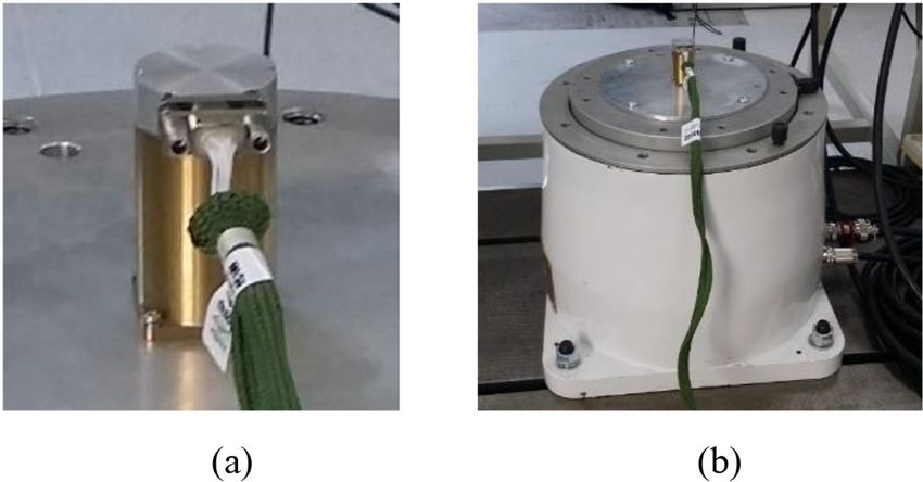
K. Wang et al.: Int. J. Metrol. Qual. Eng. 12, 2 (2021)                                   3

Jz is the current density along z axis. According to the
Ohm’s law of the whole circuit, Jz can be calculated.

                   J z ¼ s ðEz  B  V Þ                 ð5Þ

where s is the conductivity, Ez is the vortex electric field
from the varying magnetic field induced by the varying
induced current, and B  V is the induced electric field in
the conductive fluid from the cutting magnetic wire. In
general, Ez is smaller than B  V because the induced eddy
magnetic field is lower three order of magnitudes than the
permanent field B. The profile of the flow velocity V
relative to the magnetic field can be formulated as
                               y
                   V ¼ vs  v ¼ vi  v                   ð6Þ
                               r
where, when y = r, v = vi and when y = R, v = vi  R/r.                         Fig. 3. Mechanism diagram.
From equations (4)–(6), we can get
                            y
                 F em ¼ B2 s vi  v                 ð7Þ
                             r
                                                               formulated as
   Substituting equation (7) into equation (3), the
dynamic equation can be formulated.                                               U z ðsÞ                 s
                                                                         GðsÞ ¼           ¼ BlrRMS     n                ð13Þ
                              y                                               vi ðsÞ           s þ 2 1 þ M2
              dv         1
            r ¼ 1 þ 2 B2 s vi  v               ð8Þ                                                   h
              dt        M        r
                                                                               rffiffiffiffiffiffiffiffiffiffiffi
                                                                                  R               qffiffiffiffiffiffiffiffiffiffiffiffiffiffiffiffiffiffiffiffi
where vi = rvi.                                                                 ∫r y2 dy           ðR2 þRrþr2 Þ
                                                               where rRMS ¼         Rr       ¼              3
   After the Laplace Transformation, we get
                            y
                        1
         rsvðsÞ ¼ 1 þ 2 B2 s vi ðsÞ  vðsÞ               ð9Þ   3 Design and analysis
                      M         r

   So, we can get v                                            According to the schematic diagram as shown in Figure 1a,
                                                               the mechanism is designed as shown in Figure 3. This is a
                   y                  1                        2D plane drawing, and the 3D model can be got by rotating
             vðsÞ ¼ vi ðsÞ       rs                     ð10Þ   around the axis. Magnetic flux from permanent 1 passes
                   r                 þ1
                              2     1                          through magnetizer 1, magnetizer 2, hydrargyrum,
                             B s 1þ 2                          magnetizer 3, magnetizer 4, in turn, and finally reaches
                                   M
                                                               to permanent 1. Another magnetic flux from permanent 2
   Then the output voltage Uz can be formulated                with opposite magnetic field direction configuration also
                                                               passes through the hydrargyrum in the same direction. The
                                y
                                                               designed total height is 26 mm and the height of
         U z ðsÞ ¼ BlV ðsÞ ¼ Bl vi ðsÞ  vðsÞ
                                 r                             hydrargyrum is 15 mm. The radius is 13 mm, and the
                     y               s                         inner radius of the hydrargyrum loop is 9.6 mm and the
                ¼ Bl vi ðsÞ                          ð11Þ    thickness of the hydrargyrum loop is 1.4 mm. The design
                     r          B2 s      1                    can get the radial magnetic field shown in Figure 1b.
                             sþ       1þ 2
                                 r       M                         Electrodes are installed between the top and the bottom
                                       qffiffiffiffi                   of the hydrargyrum loop and connected through the
                                          s
   Because vi (s) = rvi (s) and M ¼ Bh rn    , the relation    conductive pillar along the axis as shown in Figure 3. The
                                                               circuit of hydrargyrum loop, electrodes and conductive
between Uz (s) and vi (s) can be formulated. Here, n is the
                                                               pillar can be seen as a primary coil of the transformer.
dynamic viscosity coefficient of the liquid, h is half of the
                                                               Another coil is installed coaxially with the conductive pillar
width of hydrogarum loop as shown in Figure 2 [22].
                                                               as the secondary coil of the transformer. This transformer is
               U z ðsÞ             s                           used to isolate and amplify the signal of the hydrargyrum
                       ¼ Bl     n       y             ð12Þ   loop.
               vi ðsÞ       s þ 2 1 þ M2
                               h                                   The design prototype’s parameters are shown in
                                                               Table 1.
where y changes from r to R, it can take the mean square           Here, rRMS = 10.31 mm andM = 15.65. From Table 1,
root of R and r. Then, the transfer function can also be       the transfer function can be recalculated by equation (13)
4 K. Wang et al.: Int. J. Metrol. Qual. Eng. 12, 2 (2021)
Table 1. The designed prototype’s parameters.
Parameter Symbol Value Unit
Magnetic flux density B 0.7 T
Height of hydrogarum loop l 15 mm
Inner radius of hydrogarum loop r 9.6 mm
Outer radius of hydrogarum loop R 11 mm
Width of hydrogarum loop h 0.7 mm
Dynamic viscosity coefficient@20 °C n 7.5 108 m2/s
Hydrogarum density r 13.6 103 kg/m3
Conductivity@20 °C s 1.04 106 s/m
Fig. 4. Frequency characteristics of MHD angular vibration sensor. (a) Amplitude-frequency responses. (b) Phase-frequency
responses.
as the following. It can be found that within ±10%, the magnetic flux
density B and the height of the hydrogarum loop l, the
1:082 104 s inner radius of hydrogarum loop r and the outer radius of
GðsÞ ¼ ð14Þ the hydrogarum loop R are all positively correlated with
s þ 37:624
the amplitude. However, their influence on the amplitude is
different. B and l have the strongest influence, r is less, and
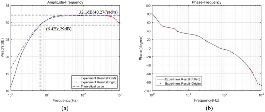
According to equation (14), the amplitude-frequency
R is the least. In addition, B significantly influences the
characteristic and the phase-frequency characteristic are
corner frequency. When B increase 10%, the corner
shown in Figure 4a and b, respectively. It can be found that
frequency increase 20.5%. But l, r and R have no relevance
the sensor reveals a high pass feature. The corner frequency
to the corner frequency. The detailed values are listed in
is about 6.0 Hz with 3 dB attenuation. The output
Table 2.
signal’s amplitude is about 108 mV/rad/s. Figure 4b shows
that the phase changes from 90° to 0. The phase invert
center is 45° at 6.0 Hz. 4 Experiments
Several adjustable parameters related to the design are
selected to explore the amplitude-frequency character- The measuring circuit of the sensor is shown in Figure 6.
istic’s sensitivity. These parameters include B, l, r, and R. The signal from the hydrargyrum loop is isolated and
When one parameter is adjusted to be an alternation amplified through the transformer, then amplified again by
of ±5% or ±10%, the other parameters are not changed, an instrumentation amplifier, finally filtered by an active
taking values according to Table 1. Each parameter’s second-order low-pass filter with the cut-off frequency of
influences to the frequency amplitude are shown in Figure 5. 1200 Hz.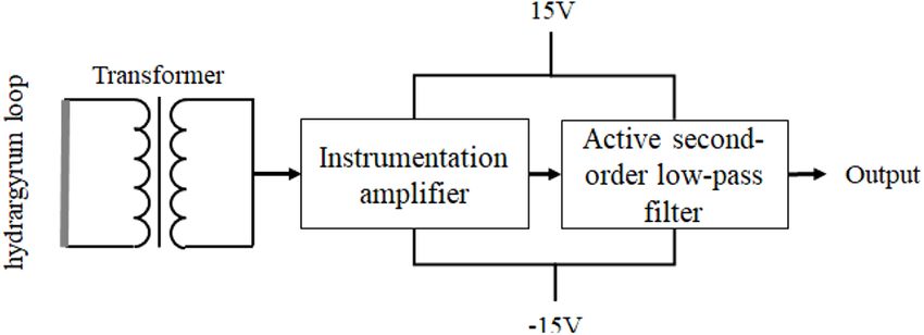
K. Wang et al.: Int. J. Metrol. Qual. Eng. 12, 2 (2021)                                 5

Fig. 5. The amplitude-frequency characteristic’s sensitivity analysis to micro adjustment of the designed parameters. (a) B
adjustment; (b) l adjustment; (c) r adjustment; (d) R adjustment.

Table 2. Amplitude and corner frequency changing to parameter alteration.

Characteristics                      Parameter           10%           5%             0            5%             10%
                                     B                    9.741         10.282          10.823       11.364         11.906
                                     l                    9.741         10.282          10.823       11.364         11.906
Amplitude (105 V/rad/s)            r                   10.336         10.578          10.823       11.071         11.320
                                     R                   10.238         10.529          10.823       11.119         11.418
                                     B                    4.85           5.41            6.00         6.59           7.23
                                     l                    6.00           6.00            6.00         6.00           6.00
Corner frequency (Hz)                r                    6.00           6.00            6.00         6.00           6.00
                                     R                    6.00           6.00            6.00         6.00           6.00
6 K. Wang et al.: Int. J. Metrol. Qual. Eng. 12, 2 (2021)
Fig. 6. Measuring circuit.
The scale factor of the prototype is designed to be about Fig. 7. (a) Prototype of the MHD angular vibration sensor;
40 V/rad/s. As shown in Figure 4, the maximum output of (b) Prototype on Angular Vibration Table.
the hydrargyrum loop is 108 mV/rad/s, so the total
magnification of the measuring circuit is designed as
370 000. Then the maximum scale factor can be calculated characteristic of the sensor prototype performs as a band-
by 108m 370 000 = 39.96 V/rad/s, close to the target. The pass filter, and the maximum scale factor is about 40.2–
prototype of the MHD angular vibration sensor has been 40.5 V/rad/s. Thus, the lower-cut-off frequency (3 dB) is
made according to the above parameters and the structural about 6.4 Hz, and the scale factor at 1000 Hz, which is still
design as shown in Figure 7a. in the pass band.
The prototype has been experimented under the The experiment shows that the lower-cut-off frequency
frequency of 1–1000 Hz to test the performance of of this MHD prototype is about 6.4 Hz, which has an 6.7%
frequency characteristics as shown in Figure 7b. Since error rate. This delay is speculated due to the transformer.
the angular vibration table used in the experiment can only From Figure 8a, it can be seen that the scale factor has a
measure under 1000 Hz, the experiment can be only significant downward trend at 1000 Hz, but still in the pass
implemented up to 1000 Hz. band. This is due to the active second-order low-pass filter.
The angular vibration used in the experiment is a sine So, it can be estimated that the upper-cut-off frequency is
wave with 0.174 rad/s (10°/s) Vpp. The original voltage not higher than the 1200 Hz, the cut-off frequency of the
signal of the sensor of every frequency point is sine fitted by low-pass filter. The max scale factor of this prototype is
40.5 V/rad/s, which is about 1.4% error from the designed
u ¼ C u ðcosð2pf⋅t þ fu ÞÞ þ Du ¼ Au cosð2pf⋅tÞ 39.96 V/rad/s. This error may be caused by various factors,
þBu sinð2pf⋅tÞ þ Du ð15Þ such as noise, resistance accuracy in the circuit, etc.
where u denotes the original voltage signal of the sensor, f is 5 Conclusion
frequency, t is time, Au, Bu, Cu, Du are corresponding
coefficients, then the output amplitude of the sensor Cu and This paper first derives the transfer function of the angular
the initial phase ’u are vibration response of the conductive fluid in the static
8 magnetic field. Then, the magnetic field and electric circuit
>
> 1 Bu
< tan ; Au ≥ 0
qffiffiffiffiffiffiffiffiffiffiffiffiffiffiffiffiffiffi > model of the sensor is designed. The model is designed as a
2 2
Au high-pass filter with a cut-off frequency of 6 Hz. Based on
C u ¼ Au þ Bu ; ’u ¼
>
> Bu this model, the sensitivity of the design parameters of
>
: tan1 þ p; Au 0 magnetic field intensity, conducting fluids’ height and
Au width are analyzed to get the optimized parameter for
ð16Þ higher precision and width. After that, a prototype,
The scale factor S ^ and phase delay Df _ can be including the measuring circuit, was developed to verify
u_ u
calculated by the analysis and optimization. Finally, the experiment
is implemented to get the frequency characteristics of
u^ 180
1–1000 Hz. The result shows that the cut-off frequency of
S ^ ¼ ; Df _ ¼ ⋅ fu f _ ð17Þ
u_ ^u_ u p u the prototype increases from 6 Hz of the model to 6.4 Hz,
and the error is about 6.7%. the max error in scale factor is
where u^_ and f _ are the angular vibration amplitude and about 1.4%, which from 39.96 to 40.5 V/rad/s. These errors
u
the initial phase of the angular vibration, respectively. are within the acceptable, and the results can verify the
The frequency characteristics of this prototype can be model proposed in this paper. The experiment shows that
drawn according to the experiment results on the angular the prototype meets the design requirement of 6–1000 Hz,
vibration table. The sensor’s amplitude-frequency charac- and the model is accurate.
teristic and phase-frequency characteristic curve are shown However, this MHD angular vibration sensor still needs
in Figure 8a and b, respectively. In addition, the theoretical some improvements. The current MHD prototype cannot
amplitude-frequency curve of the model is the blue line in measure low-frequency angular vibration signals below
Figure 8a. It can be seen that the amplitude-frequency 6 Hz. The traditional gyroscope is needed to be used withK. Wang et al.: Int. J. Metrol. Qual. Eng. 12, 2 (2021) 7
Fig. 8. Frequency characteristics of MHD sensor prototype in experiment. (a) Amplitude-Frequency; (b) Phase-Frequency.
this sensor prototype to complete angular vibration 6. H. Alfvén, Magnetohydrodynamic waves in the atomic
measurements within 0–1000 Hz. This is mainly because nucleus, Phys. Rev. 107, 632–632 (1957)
a larger magnetic flux density B is used to improve the 7. E. Egorov, V. Agafonov, S. Avdyukhina, S. Borisov, Angular
signal-to-noise ratio, the output of sensor and reduction molecular-electronic sensor with negative magnetohydrody-
circuit amplification, which leads to a higher cut-off namic feedback, Sensors 18, 245 (2018)
frequency in the model. In addition, the transformer in the 8. M. Anwari, Effect of magnetic field on a Diagonal MHD
measuring circuit also increases the cut-off frequency. In Accelerator, 2008 IEEE Vehicle Power and Propulsion
the future research, a transformer with better low- Conference, IEEE, 2008, pp. 1–5
frequency performance should be selected to decrease the 9. D.R. Laughlin, Magnetohydrodynamic (MHD) actuator
sensor. Google Patents (2007)
cut-off frequency, and the measuring circuit should be
10. D. Laughlin, H. Sebesta, D. Eckelkamp-Baker, A dual
modified to improve the detection and amplification of
function magnetohydrodynamic(MHD) device for angular
weak signals. As a result, a smaller magnetic flux density B motion measurement and control, Adv. Astronaut. Sci. 111,
can be used to decrease the cut-off frequency of the sensor. 335–347 (2002)
In addition, noise and the accuracy of circuit components 11. T. Iwata, Precision on-board orbit model for attitude control
also should be concerned to decrease the error. of the advanced land observing satellite (ALOS), J.
Aerospace Eng. 4, 62–74 (2012)
References 12. A. El-Osery, S. Bruder, D. Laughlin, High-accuracy
heading determination, 2013 8th International Conference
1. D.R. Laughlin, D. Smith, Development and performance of on System of Systems Engineering, IEEE, 2013, pp.
an angular vibration sensor with 1-1000 Hz bandwidth and 308–313
nanoradian level noise, Free-Space Laser Communication 13. B. Ando, S. Baglio, A. Beninato, A low-cost inertial sensor
and Laser Imaging, Int. Soc. Opt. Photonics 4489, 208–214 based on shaped magnetic fluids, IEEE Trans. Instrum.
(2002) Meas. 61, 1231–1236 (2012)
2. M. Sohail, Modified heat and mass transmission models in the 14. H.E. Shimin, T. Liang, High-bandwidth measurement
magnetohydrodynamic flow of Sutterby nanofluid in stretch- based attitude determination, Aerospace Control Appl. 37,
ing cylinder, Phys. A Stat. Mech. Appl. 549, 124088 (2020) 20–25 (2011)
3. R.V.M.S.S. Kiran Kumar, S. Vijaya Kumar Varma, C.S.K. 15. H. Huo, M. Ma, Y. Li, J. Qiu, The application of MHD
Raju, S.M. Ibrahim, G. Lorenzini, E. Lorenzini, Retraction angular rate sensor in aerospace, Vac. Cryogenics 17,
Note to: Magnetohydrodynamic 3D slip flow in a suspension 114–120 (2011)
of carbon nanotubes over a slendering sheet with heat source/ 16. H. Huo, M. Ma, Y. Li, J. Qiu, High precision measurement
sink, Contin. Mech. Thermodyn. 29, 1–17 (2019) technology of satellite’s angle microvibration, Transducer
4. S. Jimenez-Flores, J.G. Pérez-Luna, J.J. Alvarado-Pulido, Microsyst. Technol. 3, 4–6 (2011)
A.E. Jiménez-González, Development and simulation of a 17. M. Xu, X. Li, T. Wu, X. Yu, C. Chen, Structure design and
magnetohydrodynamic solar generator operated with NaCl experiment study for MHD gyroscope, Chin. J. Sci. Instrum.
electrolyte solution, J. Solar Energy Eng. 143, 1–9 (2020) 36, 394–400 (2015)
5. C.R. Evans, J.F. Hawley, Simulation of magnetohydrody- 18. Y. Wu, X. Li, F. Liu, G. Xia, An on-orbit dynamic calibration
namic flows a constrained transport method, Astrophys. J. method for an MHD micro-angular vibration sensor using a
332, 659–677 (2007) laser interferometer, Sensors 19, 4291 (2019)8 K. Wang et al.: Int. J. Metrol. Qual. Eng. 12, 2 (2021)
19. Y. Ji, G. Yan, Y. Du, Low-frequency extension design of 21. Y. Ji, X. Li, T. Wu, J. Wu, Preliminary study on the
angular rate sensor based on magnetohydrodynamics, magnetohydrodynamic (MHD) angular rate sensor combing
2020 IEEE 5th Information Technology and Mechatronics coriolis effect at low-frequency, 2017 IEEE 3rd Information
Engineering Conference (ITOEC), IEEE, 2020, pp. Technology and Mechatronics Engineering Conference
182–186 (ITOEC), IEEE, 2017, pp. 210–214
20. Y. Ji, M. Xu, X. Li, T. Wu, W. Tuo, J. Wu, J. Dong, Error 22. R. Moreau, S. Molokov, H.K. Moffatt, Julius Hartmann
analysis of magnetohydrodynamic angular rate sensor and his followers: a review on the properties of the
combing with coriolis effect at low frequency, Sensors 18, Hartmann layer, in: Magnetohydrodynamics, Springer,
1921 (2018) 2007, pp. 155–170
Cite this article as: Kundong Wang, Youwei Ma, Jianming Wu, Qinghua Zhu, Yue Gu, Hongli Qi, Design parameters analysis
and verification of angular vibration sensor based on magnetohydrodynamics, Int. J. Metrol. Qual. Eng. 12, 2 (2021)You can also read