Detection of Multidecadal Changes in Vegetation Dynamics and Association with Intra-annual Climate Variability in the Columbia River Basin
←
→
Page content transcription
If your browser does not render page correctly, please read the page content below

Detection of Multidecadal Changes in Vegetation Dynamics
                                            and Association with Intra-annual Climate Variability in the
                                            Columbia River Basin
                                            Andrew B Whetten 1 , Hannah Demler     2
arXiv:2105.08864v1 [q-bio.QM] 19 May 2021

                                            1 Department of Mathematical Sciences, University of Wisconsin-
                                            Milwaukee, WI
                                            2 USDA ARS Ainsworth Research Lab, University of Illinois - Urbana
                                            Champaign, IL

                                            * awhetten@uwm.edu

                                            Abstract
                                            Leaf Area index is widely used metric for the assessment of vegetation dynamics and
                                            can be used to assess the impact of regional/local climate conditions. The underlying
                                            continuity of high resolution spatio-temporal phenological processes in the presence of
                                            extensive missing values poses a number of challenges in the detection of changes at a
                                            local and regional level. The feasibility of functional data analysis methods were
                                            evaluated to improve the exploration of such data. In this paper, an investigation of
                                            multidecadal variation of leaf area index (LAI) is conducted in the Columbia Watershed,
                                            as detected by NOAA AVHRR satellite imaging, and its inter- and intra-annual
                                            correlation with maximum temperature and precipitation using the ERA-Interim
                                            Reanalysis from 1996 to 2017. A functional cluster analysis model was implemented to
                                            identify regions in the Columbia Watershed that exhibit similar long-term greening
                                            trends. Across these several regions, the primary source of annual LAI variation is a
                                            trend toward seasonally earlier and higher recordings of regional average maximum LAI.
                                            Further exploratory analysis reveals that although strongly correlated to LAI, maximum
                                            temperature and precipitation do not exhibit clear longitudinal trends.

                                            1    Introduction
                                            Understanding how changing climate conditions interact with and affect the biosphere is
                                            necessary for characterization of global change and for developing and implementing
                                            adaptive and sustainable practices worldwide. The study of ecological responses to
                                            climate change has greatly expanded in the recent past with the development and use of
                                            remote sensing and the compilation of multidecadal satellite data sets. Satellites allow
                                            for near continuous observations of earth and monitoring of changes in the biosphere on
                                            scales ranging from local to global [1].
                                                Plant life serves a critical role globally in regulating energy, chemical, and mass
                                            transfers within the earth system and changes in vegetation at different scales effects
                                            land surface - climate system feedbacks and ecosystem services through regulation of
                                            carbon, water, and energy exchanges between the atmosphere and biosphere [2, 3].
                                            Many studies have reported a ”greening” of the planet attributed to the ”fertilization
                                            effect” of higher atmospheric [CO2 ], nitrogen deposition, or increasing temperatures

                                                                                                                               1/25
lengthening the growing season in many regions [4–6]. However, complex interactions
exist between plant physiology, atmospheric conditions, temperature, and water and
nutrient availability that make the picture of how plants respond to changing climate
conditions less clear [7, 8].
    Phenology refers to periodic and seasonal reproductive events in biological life cycles.
Vegetative phenological phenomena are sensitive to annual climate conditions and
therefore changes in phenology, such as the timing, rate, duration, and magnitude of
annual vegetative growth, can signal important effects of climate change on plants [9].
Leaf Area Index (LAI), a widely utilized measure of plant growth and activity, is a
unit-less measurement of leaf area (m2 ) per ground area (m-2 ). LAI provides a key
measure of plant cover in a given area and is defined as an essential climate variable
(ECV) by the Global Climate Observing System (GCOS) due to its critical contribution
to the characterization of Earth’s climate [10]. Satellite-derived LAI products offer
multidecadal records of terrestrial plant cover around the world, allowing for analysis of
inter-annual variability in vegetation dynamics which provides key insight to how plants
respond to global change.
    Earth-observing satellites have used greening indices to infer phenological changes
and vegetation stress since the early 1980’s and in recent decades the quality of these
products has continued to improve. These improvements have yielded massive reservoirs
of high resolution spatio-temporal data [11]. Remotely sensed vegetation data poses a
number of challenges. (1) The regular and dense occurrence of missing values resulting
from excessive cloud cover, snow cover, and barren landscapes requires extensive
pre-processing of the data. (2) For the analysis of large regions, tens of thousands of
sites are available. The analysis of thousands of adjacent sites requires modeling of the
inherently complex spatio-temporal correlatory structure. (3) The collection of a
phenological process over multiple decades yields many replications of a stochastic
process at each site. The variability of intra-site replications of an annual process is
often characterized by complex cyclic or at least year-dependent structure.
    This analysis is motivated by the recent work to detect summer NDVI greening
patterns in the Arctic Tundra Biome conducted by the GEODE Lab at Northern
Arizona University [12]. Their work utilizes maximum recorded greenness at a given site
annually, as measured by NDVI, to detect greening or browning trends across 50,000
sites in the Arctic tundra. To the best of our knowledge, most literature on the analysis
of greening trends rely heavily on the annual maximum or mean greenness trends using
time series and temporal site/region correlation [13–15].
    The variations of this approach have a number of advantages. Maximum/mean
greenness is by far the most important phenological attribute, and the dimensionality of
the data is decreased exponentially as measurements throughout the remainder of the
years are filtered out. Further, the expansive number of missing values inherently
present in such data are removed. These are all advantageous and justifiable
simplifications that ameliorate subsequent statistical analysis.
    This simplification neglects modeling the elegant periodicity and continuity of plant
phenology. Further, it limits the potential of an effective exploratory analysis of such
data products. In this project, a philosophically different approach is taken to analyze
remotely sensed phenological data in which the unit of analysis is a curve (or function)
as opposed to a single site measurement. This approach, widely referred to as functional
data analysis (FDA) roots in the assumption that measurements vary over some
continuum such as space or time and that there is an underlying smoothness inherent to
the process of interest [16–18]. A temporal process, measured discretely on a regular or
irregular time grid, is smoothed using an optimized basis function expansion. In almost
all circumstances, replications of this process are present at the same spatial location or
across several different locations, and as such, a collection of continuous differentiable

                                                                                      2/25
curves are obtained for analysis.
    The retention of an entire smooth curve yields several advantages for vegetation
dynamics applications: (1) Missing values can be effectively smoothed over, (2)
Anomaly values can be filtered/smoothed out of the data, (3) the timing of the
magnitude of max greenness is retained naturally/simultaneously, and (4) differential
information is naturally contained in the basis function expansion used to smooth the
curves. Literature documenting the use of FDA in remotely sensed plant phenology is
sparse, but recent work in mapping forest plant associations using FDA combined with
other machine learning methodology has shown promising results [19].
    The Columbia River Basin (CRB) is located in the north-western United States and
south-western British Columbia, Canada.The drainage basin is bounded by the Rocky
Mountains to the east and the Cascade and Coast ranges to the west and covers and
area of 670,000 km2 : 568,000 km2 of which are spread across the US states of
Washington, Oregon, Idaho, Montana, Wyoming, Utah, and Nevada. Climate in the
CRB varies from humid and maritime along the western parts of the basin to semi-arid
and arid in the southeast. The CRB hosts a range of diverse natural ecosystems as well
as large agricultural regions consisting largely of forestry, dairy and cattle farming, and
production of apples, potatoes, wheat, and other small grains. (USGS River Basins of
the United States: the Columbia report).
    In this project, a cluster analysis is performed on 27,196 sites in the CRB that
incorporate pairwise site correlations between smoothed multidecadal LAI site profiles
from 1996-2017 remotely sensed using NOAA AVHRR times series product. Intuitive
clusters were detected that are largely distinguished by land cover, elevation, the
seasonal timing and magnitude of peak LAI. Further, substantial regional inter-annual
variation is identified across several clusters that is explained by earlier and increasing
magnitude of maximum LAI. We supplement this work with an exploratory applet that
can be accessed from Supporting File S2.
    Using an ERA-Interim data product, strong correlations were detected between
intra-annual temperature profiles characterized by warmer temperatures during the first
20 weeks of the year and the timing and magnitude of LAI throughout the CRB region.
However, Inter-annual trends in temperature over the studied time period do not match
the clear long term changes detected in LAI. Variation in precipitation profiles was not
uniformly correlated with timing and magnitude of LAI in the CRB region.
    These results provide an innovative framework for future analysis of remotely sensed
data products using functional data and spline smoothing methods, and provides
further confirmation of greening trends observed across the world in recent decades.

2     Materials and Methods
2.1    LAI AVHRR Climate Data Record
The LAI Climate Data Record (LAI CDR) produces a daily product on a 0.05 degree x
0.05 degree grid dating back to 1981 derived from Advanced Very High Resolution
Radiometer (AVHRR) sensors using data from eight NOAA polar orbiting satellites:
NOAA -7, -9, -11, -14, -16, -17, -18 and -19. The highest resolution of AVHRR sites is
approximately 1km per pixel [20, 21]. In this analysis, we subset the data from January
1st, 1996 until December 31st, 2017 and the spatial domain is restricted to 37,110 sites
in the US portion of the CRB (refer to Fig 2). In this 22-year period, daily LAI
measurements are summarized on a weekly resolution, by taking weekly average LAI
across a 7 day period. The resulting data product has 1152 weeks. In this product,
there are thousands of sites that report high volumes of missing values. In order to
construct spline smoothed curves on the 22 year period, a minimum threshold was set

                                                                                     3/25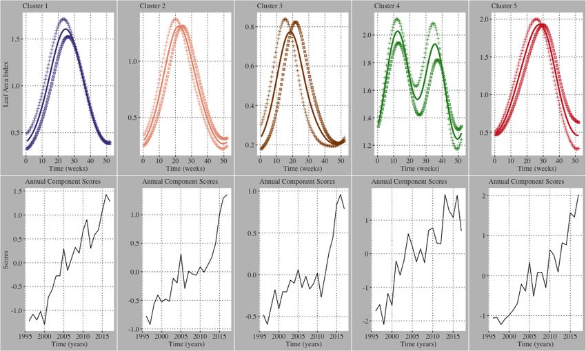
for 28 percent of weeks in the 22 year period to have at least one weekly recording of
LAI. This filtering process leaves 27196 sites. By inspection, it is clear than many sites
of the removed sites are barren/sparsely vegetated regions and high altitude sites, but
we are not certain of the quality of the products in the regions where high densities of
sites report excessive missing values. From these results, it appears that this approach is
robust enough to handle sites with higher occurrences of missing values (towards a
threshold of 15 to 20 percent), although this is left to future work.

2.2    ERA-Interim Reanalysis
The ERA-Interim is a reanalysis of the global climate attributes covering the data-rich
period since 1979 (originally, ERA-Interim ran from 1989, but the 10 year extension for
1979-1988 was produced in 2011), and continuing in real time until its discontinuation
in 2019 [22]. The spatial resolution of the data set is approximately 80 km and provides
daily recordings of maximum temperature, minimum temperature, and precipitation.
[The product used in this analysis has been pre-processed into longitudinal attributes of
these climate attributes by Jupiter Intelligence (for the ENVR 2021 Data Challenge)].
This product is subsetted temporally to the same domain prescribed for the LAI CDR.
The spatial domain for this product is restricted to a square region containing the
subsetted points from the LAI CDR with the following boundaries
(Latmin = 40.5N, Latmax = 49.0N, Lonmin = −108.0W, Lonmax = −124.0W ).
Requiring that the subsetted LAI CDR product fully contained within the subsetted
ERA-Interim product is optimal for appropriate spatial prediction of climate attributes
of the ERA-Interim product onto the LAI CDR coordinate system.

2.3    BaseVue 2013 Land Cover and USGS National Elevation
       Products
The results of the cluster analysis prompted further investigation into site
characteristics that may be driving factors in the separation of clusters. We use the
BaseVue 2013 Land Cover product, which is a commercial global, land use/land cover
product developed by MDA [23, 24]. BaseVue is independently derived from roughly
9,200 Landsat 8 images and has a spatial resolution of 30m. The capture dates for the
Landsat 8 imagery range from April 11, 2013 to June 29, 2014, and contains 16 classes
of land use/land cover. Elevations were extracted at each site using the USGS National
Elevation product. This dynamic image service provides numeric values on a 30m
resolution representing orthometric ground surface heights (sea level = 0) which are
based on a digital terrain model (DTM).

2.4    Smoothing LAI
For a collection of raw weekly average recording of LAI, denoted by Y = [→      −
                                                                                y 1 ...→
                                                                                       −y n ],
                     PK
we estimate x̂(t) = k=1 ck φk (t) subject to a roughness penalty on the second
derivative of the basis expansion Φ = [φ1 (t) . . . φK (t)] where ck are the coefficients of
the terms of the basis expansion denoted by φk . This can be expressed as an
unconstrained minimization defined by

                             min
                              →
                              −
                                 k→
                                  −
                                  y − Φ→
                                       −c k2 + λcT Rc f or λ ≥ 0,                          (1)
                              c

              PM        00   ∼    00   ∼           ∼      ∼
where Rjk =      l=1   φj ( t l )φk ( t l )h for h = t l − t l−1 [16].

                                                                                          4/25
We select an appropriate value for λ coordinates using the optimal lambda for a
single site determined by the generalized cross-validation criteria, GCV = M SE(λ)
                                                                              dfλ . This
                                                                              (1−   M   )
is justifiable since the roughness of LAI recording at all sites are similar, and the
roughness penalty restriction permits the estimated functions to characterize the same
types of features across coordinates in the Columbia Watershed. The resulting
smoothed LAI curves have the form

                         x̂ = Φ(ΦT Φ + λR)−1 ΦT →
                                                −
                                                y = S→
                                                     −
                                                     y.                                      (2)

In the upper plot of Fig 1, we present an example of a smoothed 22-year LAI profile.
We emphasize that the curves retain the timing and structure of the raw data while
naturally filtering out singleton anomaly values that yield false maximum LAI readings.

Figure 1. Illustration of the LAI smoothing process. (Upper) Raw and B-spline
smoothed LAI splines overlayed for Site X (42.325N -109.775W): The spline model
retains the functional structure of the raw LAI recording while filtering out anomaly/false
recordings. (Lower Left) Spline smoothed LAI for adjacent sites: Site X and Site Y
(42.325N -109.825W). The spearman correlation is 0.988. Site X Elevation = 2133.8m
and Site Y Elevation = 2168.8m, and both sites are classified as Scrub/Shrub locations.
(Lower Right) Spline smoothed LAI for Site X and Site Z (47.425N -118.225W). The
spearman correlation is 0.769. Site Z Elevation = 690.5m and is classified as an agriculture
location [25, 26].

2.5    Spatial Clustering of High Dimensional Functional Data
Consider each smoothed curve, xˆj (t) as a vector of measurements. The pairwise
correlation of x̂j (t) with x̂j 0 (t) can be measured by plotting the two curves against each
in R2 . Plotting smoothed LAI curves in this way yields ellipsoidal paths of time-paired
LAI recordings (x̂j (ti ), x̂j 0 (ti )). We measure the strength of monotonicity of the
ellipsoidal relationship of coordinates rather than its linearity. To accomplish this, we
compute Spearman rank correlations defined by

                                                                                            5/25
Pn
                             Sx̂j x̂j0          n−1    [R(xj ) − R(xj )][R(xj 0 ) − R(xj 0 )]
ρ(x̂j , x̂j 0 ) = ρjj 0 =                =q                                                           (3)
                            Sx̂j Sx̂j0           n                          Pn
                                            n−1    [R(xj ) − R(xj )]2 · n−1
                                                P
                                                                               [R(xj 0 ) − R(xj 0 )]2

between all pairs of coordinates where R(xj ) is the ranking function of the elements of
x̂j (t). This approach proves advantageous in this application since Spearman
correlation is a computationally efficient measure of association for a high dimensional
quantity of paired coordinates. This approach also provides a notion of standardization
of the measure of association which is of great application-based importance, namely
that coordinates grouped in the same cluster have increasingly synchronous greening
patterns independent of the differences in the magnitude of LAI at each site. (As an
example, coordinates on north facing slopes may experience lower and seasonally
delayed LAI than south facing slopes, but if close enough in proximity the regularity of
paired ellipsoidal LAI movement in R2 will likely be high.
     The ρjj 0 can be thought of as a discretization of a spatial correlation function P
where ρjj 0 = P (xj , xj 0 ). The availability of longitudinal recordings of LAI at each
coordinate allows for direct estimation of ρjj 0 without placing assumptions on P [27].
The computed nxn matrix of pairwise correlations is used to construct a dissimiliarity
matrix with elements djj 0 = 1 − ρjj 0 .
     By construction, pairs of coordinates with high spearman correlation have low djj 0
values, and as such, they are considered to be close in “distance” to each other. We
then perform k-mediod clustering using the partitioning around mediods algorithm
(PAM) for k = 2, . . . , 6 clusters [28].

2.6      Ordinary Kriging of the ERA-Interim
Since the ERA-Interim reanalysis product is on an 80km resolution, spatio-temporal
prediction onto the LAI CDR grid is required. This is accomplished using Ordinary
Functional Kriging on the ERA-Interim. Considering a functional random process
{XS : s ∈ D ⊂ Rd } with d = 2 such that XS is a functional random variable for any
s ∈ D observed at n sites [29, 30]. It is assumed that the random process is second order
stationarity and isotropic. Attempting to predict a complete smooth function
X̂S0 : [a, b] → R, expressed by

                                            n
                                            X
                                   X̂S0 =          λi XSi , λ1 , . . . , λn ∈ R.                   (4)
                                             i=1

     By construction, X̂S0 is a linear combination of observed curves with weights
λ1 , . . . , λn ∈ R. Curves from locations closer to the prediction site are constructed to
have increased influence on the prediction. We use a parametric estimated
trace-semiovariongram with the exponential distribution to obtain the kriging weights
λi .

2.7      Interannual Regional LAI and Climate Variation
         Monitoring
Having obtained smoothed weekly average LAI, average maximum temperature, and
precipitation curves from 1996 to 2017 on the 0.05x0.05 degree grid, the 22 year profiles
were averaged by cluster to obtain regional average curves for the respective variables.
Subsequently, the 22 year profiles were decomposed into a collection of 22 annual curves.
The deconstruction into annual curves provides the needed replications of curves to

                                                                                                 6/25
assess interannual variation. For a given collection of average annual profile for a given
cluster LAI, denoted by X̄ˆi (t), and the Karhumen-Loeve decomposition of the annual
profiles can be expressed using the random variable Z defined by

                                                                       ∞
                                                                       X
                                                       X(t) = µ(t) +         zk ξk (t),                         (5)
                                                                       k=1

where µ is the known average profile, the ξk are orthonormal eigenfunctions that
characterize variance of individual years from the mean, and the zk are uncorrelated
random variables such that E(zk ) = 0 and V (zk ) = λk where λk is the eigenvalues
corresponding to the k th eigenfunction [16, 17]. The eigenfunction pairs ξk , known as
functional princpal components, arePthe leading eigenfunctions of the functional
                                       n
covariance defined by v(s, t) = n−1 i=1 (xi (s) − x̄(s))(xi (t) − x̄(t)) and zk is an
eigenvector of the Gram matrix G, defined by Gij =< xi − x̄, xj − x̄ > with eigenvalues
nλk .

2.8     Interannual Canonical Correlation Analysis between LAI
        and Climate Attributes
Consider a sample of paired annual curves (x1 , y1 ), . . . , (xm , ym ) from (X, Y ) where X
and Y are random functions generating realizations of annual LAI and some climate
attribute (either maximum temp or precipitation). The objective is to discover
functions (ξ, η) that maximize cor(< x, ξ >, < Y, η >). Defining Z =< ξ, X > and
W =< η, Y >, gives

                                                             cov(Z, W )
                                           ρ = cor(Z, W ) = p                                                   (6)
                                                              V (Z)V (W )

where
                           Z       b   Z       b
            V (Z) =                                cov(X(s), X(t)ξ(s)ξ(t)dsdt =< ξ, cov(X(s), X(t))ξ >,
                               a           a
                   Z   b   Z   b
        V (W ) =                   cov(Y (s), Y (t)η(s)η(t)dsdt =< η, cov(Y (s), Y (t))η >, and
                   a       a
                               Z       b   Z       b
          cov(z, w) =                                  cov(X(s), Y (t)ξ(s)η(t)dsdt =< ξ, cov(X(s), Y (t))η >
                               a           a

Subsequent canonical weight functions (ξi , ηi ) are found by maximizing Equation 6
subject to

                                                          cor(< x, ξj >, < x, ξi >) = 0,
                                                   cor(< y, ηj >, < y, ηi >) = 0, and
                                                           cor(< x, ξj >, < y, ηi >) = 0
                                                                 where j = 1, . . . , i − 1.

The functional canonical correlation analysis (fcca) requires some form of regularization
to ensure meaningful weight functions (ξ, η) since they only have m constraints but as
functions have infinite degrees of freedom (unlike classical CCA) [16]. This is
accomplished by defining the smoothed sample curves using the first four functional
principal components of X and Y as the basis expansion as opposed to a standard

                                                                                                               7/25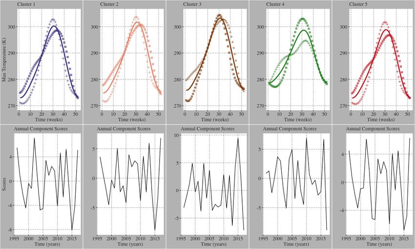
b-spline basis expansion. The fpca models have shown that the first 4 fpc’s explain 90
to 99 percent of the variability of the original sample and are expressed by
              P4        (1)                   P4        (2)
xi (t) = µx + k=1 sik νk and yi (t) = µy + k=1 sik νk where ν and sik are defined
similarly to Equation 5.
    The strength of the relationship between LAI and temperature or precipitation, ρ,
provides the conventional interpretation of correlation, but equally important, the
paired weight functions (ξ, η) are the components of variation that most account for the
interaction of the two attributes.

3    Results
This analysis detects widespread greening earlier in the growing seasons across a range
of ecosystems in the CRB from 1996 to 2017. Initial exploration of correlations between
annual maximum LAI and time in this region provide evidence of this phenological shift.
Fig 2 and Tables 1 and 2, show calculated correlations between detected annual
maximum LAI at each site and time. Significant correlations were determined at
α = 0.15. Sites that were significantly greening had positive correlations between LAI
and time, whereas sites that were significantly browning had negative correlations
between LAI and time. Non-significant correlations are denoted as neither greening nor
browning. High frequencies of greening were detected along large sections of the the
major CRB rivers (the Columbia and Snake) and in the Pacific coastal region of the
CRB. Generous significant levels were chosen in this preliminary stage since, with only
22 replications of annual maximum LAI (over the 22 years), the correlation coefficients
are sensitive to anomaly measurements and sub-intervals of decreasing annual maximum
LAI. A high anomaly reading in early years makes it difficult to detect an increasing
trend across the remaining years. Further, a sudden drop in maximum LAI in later
years may leverage the correlation away from a high positive correlation detected in
earlier intervals.

Figure 2. Temporal correlation of maximum annual LAI from 1996 to 2017 discretized
to Greening, Browning, and Neither using a significance levels of α = 0.15 [31]. Refer to
the Supporting File S2 for applet access to examine trends across this region interactively.

   The spatial distribution of greening magnitude and timing demanded a more rigorous
exploratory analysis that accomplished the following objectives: (1) eliminate/filter

                                                                                      8/25
anomalies (false high LAI recordings), (2) detect regions that are strongly correlated
over time while retaining at least some information regarding spatial proximity, and (3)
examine changes/perturbations in the functional structure of annual LAI profiles.
   A k-mediods cluster analysis was performed on the 22-year B-spline smoothed LAI
profiles using the dissimilarity matrix outlined in 2.5. Sites allocated into the same
cluster are determined to have strong multidecadal relationships to each other as
inherited from the dissimilarity matrix. Fig 3 depicts the results of the 5 cluster
k-mediods model geographically. The details of the all cluster models for k = 5 are
provided in Table 4

Figure 3. K-mediod cluster analysis of the pairwise correlation matrix of the 27191
B-spline smoothed LAI profiles [31]. Refer to the Supporting File S2 for applet access to
examine trends across this region interactively.

    The 5-clusters intuitively distinguish regions with different land cover, elevation, and
climate characteristics based on satellite-derived LAI values. Tables 1 and 2, show that
across Clusters 1, 2, 4, and 5, 32 - 70 percent of sites are identified as greening sites,
and extremely low percentages of sites in each cluster are identified as browning sites.
Table 3 shows the land cover classifications for each of the five clusters. Clusters 1,2,
and 3 contain the largest proportion of agricultural sites and the majority land cover
classification for these 3 clusters is Scrub/Shrub. Clusters 4 and 5 are dominantly
forested evergreen sites. All clusters are distinguished by significant differences in
elevation distributions, with Cluster 5 containing the highest elevation sites and Cluster
4 containing the lowest elevation sites( S1).
    Figure 4 shows annual profiles for weekly maximum LAI, weekly maximum
temperature, and average weekly precipitation for each of the five clusters. Annual
maximum LAI is highest in the evergreen forested sites in Clusters 4 and 5 and lowest
in Cluster 3, which contains sites with the highest proportion of Scrub/Shrub land cover
in the CRB. Annual temperature profiles are similar throughout the CRB region, with
slightly lower annual maximum and higher annual minimum temperatures detected
throughout the 22-year time period at the low-elevation coastal sites comprising Cluster
4. Annual precipitation profiles are similar for Clusters 1,2,3, and 5, with Cluster 4
receiving much greater cumulative precipitation than the other clusters each year.
    Functional principal components analysis on the annual LAI profiles found that
among all of the clusters, 55-75 percent of the inter-annual variation is described by the
first principal component characterized by an earlier and higher peak in annual
maximum LAI. A linear increase in principal component scores over time indicates a
trend toward earlier and higher annual maximum LAI throughout the CRB region

                                                                                       9/25
(Figure 5). This demonstrates that despite differences in land cover, elevation, and
annual precipitation profiles between the five-clusters, a clear greening trend is detected
over the 22-year period throughout the CRB. Identical analysis on annual cumulative
precipitation showed 90 percent of the inter-annual variation among all of the clusters
was explained by the first principal component characterized by either greater or less
annual cumulative precipitation. Functional principal components analysis on
temperature showed 45-48 percent of the inter-annual variability is explained by the
first principal component associated with linearly warmer temperatures from the
beginning of the year through the annual peak in summer temperatures. The second
principal component, explaining 20-23 percent of the inter-annual variability among the
five clusters, is associated with either significantly warmer temperatures during roughly
the first 20 weeks of the year and a lower annual maximum temperature, or cooler
temperatures during the first 20 weeks of the year and a higher annual maximum.
Annual maximum temperature and annual precipitation profiles do not demonstrate an
obvious trend over the time period 1996-2017 (Figure 6, 7).
    Functional canonical correlation analysis reveals correlations between intra-annual
variation in temperature and precipitation and the earlier and higher LAI peak being
detected in each of the clusters. In each cluster, the shift in phenology toward earlier
and higher annual maximum LAI values are correlated with warmer temperatures
during the first 20 weeks of the year, shown in Figure 8. Functional canonical
correlation between LAI and precipitation did not yield a consistent correlation among
the clusters. Greater and earlier maximum LAI was correlated with greater spring
precipitation in Clusters 1 and 5, and greater but not earlier maximum LAI in Cluster 3
was also correlated with greater spring precipitation, shown in Figure 9. Taken
together the results of the functional canonical correlations indicate that the widespread
shift in phenology toward an earlier and higher peak in annual LAI in the CRB is
largely associated with warmer temperatures early in the year. However, the differences
in interannual trends in temperature and LAI over the studied time period suggest
there are other drivers of the trend in LAI not captured in this analysis. Greater annual
maximum temperatures are not shown to be correlated with this shift in LAI and the
correlation between annual precipitation and the timing and height of the annual LAI
peak varies between the 5 clusters.

Table 1. Summary of Max LAI temporal correlation results.
 Regions Freq Browning Greening Neither
 Cluster 1 12548     900       4087      7561
 Cluster 2 6737      104       2646      3987
 Cluster 3 5593       82        790      4721
 Cluster 4  742        5        517       220
 Cluster 5 1571      207        547       817

Table 2. Summary of the Max LAI annual location correlation results.
 Regions Earlier Later Neither
 Cluster 1  3885     157    8506
 Cluster 2  1398     119    5220
 Cluster 3  1049      60    4484
 Cluster 4    82     102     558
 Cluster 5   349      26    1196

                                                                                    10/25
Table 3. Summary Statistics of 5-cluster model. Proportion of land cover are zonal
statistics from the MDA BaseVue 2013 Land Cover product with the coordinates of each
cluster set as the zones. Elevation is extracted for each site from the USGS Ground
Elevation digital terrain model.
Regions Freq Prop Agriculture Prop Scrub Prop Evergreen Med Elev (m
Cluster 1 12548 0.130 0.293 0.238 1451.1
Cluster 2 6737 0.161 0.455 0.155 1150.3
Cluster 3 5593 0.174 0.667 0.010 942.0
Cluster 4 742 0.009 0.241 0.481 337.8
Cluster 5 1571 0.022 0.209 0.617 1776.8
Table 4. K-mediod 5-cluster model characteristics.
Regions Freq Max Diss Avg Diss Diameter Separation
Cluster 1 12548 0.6775 0.0744 1.0174 0.0025
Cluster 2 6737 0.6746 0.0730 1.0496 0.0025
Cluster 3 5593 0.8158 0.0956 1.1354 0.0033
Cluster 4 742 0.9487 0.3087 1.2693 0.1110
Cluster 5 1571 0.8639 0.2350 1.1874 0.0035
Table 5. Percent of variation explained by the first principal component of LAI,
Maximum Temperature, and precipitation.
Regions Attribute Proportion of Variation Component
Cluster 1 LAI 0.757 1st
Cluster 2 LAI 0.639 1st
Cluster 3 LAI 0.554 1st
Cluster 4 LAI 0.647 1st
Cluster 5 LAI 0.604 1st
Cluster 1 Max Temp 0.475 1st
Cluster 1 Max Temp 0.214 2nd
Cluster 2 Max Temp 0.481 1st
Cluster 2 Max Temp 0.210 2nd
Cluster 3 Max Temp 0.482 1st
Cluster 3 Max Temp 0.198 2nd
Cluster 4 Max Temp 0.446 1st
Cluster 4 Max Temp 0.233 2nd
Cluster 5 Max Temp 0.462 1st
Cluster 5 Max Temp 0.225 2nd
Cluster 1 Precip 0.903 1st
Cluster 2 Precip 0.914 1st
Cluster 3 Precip 0.917 1st
Cluster 4 Precip 0.917 1st
Cluster 5 Precip 0.912 1st
11/25Figure 4. Interannual regional average weekly maximum LAI, maximum Temp, and
average precipitation profiles. The curves are colored on a gradient scale where greener
curves are closer to 1996 and pinker curves are closer to 2017. Noticeable time-dependent
changes in LAI were identified where no clear trend in temperature and precipitation is
visually observed.
12/25Figure 5. LAI functional principal components results for the first principal component
of each cluster. Upper plots solid lines are the mean annual profiles and the (+) markers
denote the trend line for the first component added to the mean function with an
appropriate scaling factor, and the () markers denote the trend line for the first
component subtracted from the mean function with the same scaling factor. The lower
plots visual the annual scores of the first component as a time series from 1996 to 2017.
Years with scores greater than zero are characterized by the (+) trend line and years
with scores less than zero are characterized by the () trend line.
Figure 6. Weekly maximum temperature 1st functional principal component results
for the first principal component of each cluster.
13/25Figure 7. Weekly maximum temperature 2nd functional principal component results
for the first principal component of each cluster.
Figure 8. Weekly average precipitation first functional principal component results for
the first principal component of each cluster.
14/25Figure 9. LAI vs Max. Temperature functional canonical correlation results for the first
pair of canonical weight functions. The correlation between site attributes is listed above
each columns of plots. The (+) markers denote the trend line for the first weight function
(for either the LAI weight function or the maximum temperature weight function) added
to the mean function with an appropriate scaling factor, and the () markers denote the
trend line for the first weight function subtracted from the mean function with the same
scaling factor. The strength of the correlation between LAI and maximum temperature
is characterized by examining the pair of (+)-profiles or ()-profiles across (for each site
attribute).
15/25Figure 10. LAI vs Cumulative Precipitation functional canonical correlation results
for the first pair of canonical weight functions. The correlation between site attributes
is listed above each columns of plots. The (+) markers denote the trend line for the
first weight function (for either the LAI weight function or the precipitation weight
function) added to the mean function with an appropriate scaling factor, and the ()
markers denote the trend line for the first weight function subtracted from the mean
function with the same scaling factor. The strength of the correlation between LAI and
precipitation is characterized by examining the pair of (+)-profiles or ()-profiles across
(for each site attribute).
4 Discussion
The results of this work demonstrate the utility of FDA for the detection of annual
greening trends of high dimensional phenological processes, and more specifically, the
characterization of the within-year and across-year trends in vegetation dynamics.
Annual greening of field measured or remotely sensed sites is best characterized by
multiple parameters, namely the magnitude of the peak ”greenness”, the (annual)
timing of the peak, the duration of greeness, and the point of maximum change in
greenness. Although only the first and second of these parameters are examined in this
analysis, all of these features are inherently contained in the sample of 27196 smooth
functions used in this study. Any future work to examine the other features of LAI
curves can be performed using the same preprocessing used here. Without the use of
spline smoothed LAI curves, the analysis of these individual parameters must be
assessed without the same theoretical cohesiveness present in this approach. Ultimately,
annual LAI profiles are simple to smooth, and we demonstrate that variation in annual
LAI across years is effectively detected and explained using functional principal
components analysis.
We believe that the modeling of processes with underlying continuity should take
advantage of this continuity when possible. In this analysis, we demonstrate that the
modeling of continuous processes in the presence of high volumes of missing values is
achievable, and our results lead us to believe that our choice to only consider sites with
less than 72 percent missing values is conservative, and such an analysis would be
effective with upwards of 80 percent missing values. This provides opportunities to use
such methods in regions where remotely sense greenness indices are recorded in with
16/25extreme sparseness, such as boreal, and Arctic climates. We must acknowledges
disadvantages of our sampling of sites in the region. First, the quality of the LAI
AVHRR CDR has improved in quality across its entire domain from 1982 to present.
Beginning in 1996 eliminates some of the years with the lowest quality, but it is possible
and likely that we have removed sites that had improved satellite coverage in the later
years of the domain. Also, we note that the removal of most sites along the
Montana-Idaho border and mountains of Oregon and Washington is not indicating
low-greenness but rather poor coverage through a substantial portion of years in our
study.
Our clustering approach used in this project is effective at separating regions
intuitively across an array of variables (land cover, elevation, temperature, and
precipitation) with only the use of satellite-derived LAI profiles, and further, this
provides the theoretical framework used to make regional inferences about changes in
climate and greenness. The approach is proficient for analyzing tens or hundreds of
thousands of sampled sites.
Although our cluster model retains some implicit use of proximity of sites (since
closer sites have a tendency to have higher correlations), we believe that there are
necessary improvements to such a clustering approach, namely the filtering of noise sites
(using methods such as DBSCAN) and inducing a spatially weighting (or penalization)
on the dissimilarity matrix used in our work. We argue that the merits of the approach
taken justify its presentation here, and we encourage further work in unsupervised
learning methodology of phenological processes.
We emphasize that our work here is strictly exploratory, and not predictive. The
relationships between climate and LAI discussed here are associative by nature, and
further work using functional regression models is required to explore the fascinating
predictive relationship between these attributes. Recent literature implementing
predictive modeling of fpca scores of NDVI has yielded promising results, and this
approach can be extended to model climatic factors (such as CO2 concentration, GPP,
plant respiration, Soil moisture) that predict higher fpca scores for LAI in recent years
in this region [19].
Our work is also insufficient without recognizing disadvantages of the LAI CDR
using AVHRR sensors [33–35] . Recent literature has shown that this product is lesser
to MODIS sensors in making valid inferences on field measurement resolution and areas
with higher annual precipiation (>1m) precipitation [36, 37]. As shown in Fig 4,
regional cumulative precipiation averages for all clusters are well below this threshold.
We add our work to the body of literature on the detection of changes in remotely
sensed greening, and we emphasize that the methods used in this project are directly
extendable to any remotely sensed time-series data.
In this analysis, we were able to reveal a shift in annual vegetation dynamics from
1996-2017 across a range of land cover classes and ecosystem types in the CRB of North
America. Plant phenological events in temperate regions are triggered predominantly by
the well-known climatic changes associated with the changing of the seasons. These
responses of vegetation to environmental conditions provide a measurable and accurate
signature of the impacts climate change is having on plants [38]. The importance of
understanding how plants respond to changing climate conditions has led to
considerable work on the influence of climate variables on plant phenology [39]. Our
analysis investigates the intra-annual relationships between vegetation dynamics and the
climate variables temperature and precipitation throughout the year over a
multidecadal timescale. Temperature is the dominant driver of the timing of many plant
developmental processes and phenological shifts [40–42]. Plants synchronize their
growth and development with favorable thermal conditions in order maximize the
growing season and minimize the risk of frost damage. Sufficient exposure to cold
17/25temperatures in the winter is required for many plants to break dormancy, and a
subsequent accumulation of degree days in the spring (time above a given temperature
threshold) triggers budburst and the unfolding of leaves [43].
In the present study, earlier and higher annual maximum LAI throughout the CRB
was largely correlated with higher temperatures during the first 20 weeks of the year.
Phenological responses to environmental conditions can vary significantly among
different regions and plant species [44, 45]; however, similar trends in vegetation
dynamics were found across a range of natural ecosystem and land cover types in the
CRB, indicating common responses to abiotic environmental factors across the regional
scale of this study. On agricultural land, spring planting date could influence the timing
and magnitude of the peak in annual LAI. However, each of the 5 clusters contains a
variety of land cover types and relatively small proportions of agricultural land. Because
all of the clusters are showing coherent trends in LAI over the time period studied, the
effect of differences in planting date on the agricultural fields in each cluster likely does
not significantly influence the satellite-observed regional vegetation dynamics in the
CRB.
The same intra-annual temperature trend was correlated with the earlier and higher
maximum LAI values in each of the five clusters in the CRB. This result shows that
greater accumulation of warm temperatures early in the year leads to an earlier onset of
budburst and leaf unfolding, as well as an earlier peak of plant productivity in the
summer growing season. Intra-annual trends in cumulative precipitation did not
demonstrate a uniform correlation with the observed LAI trend among the five clusters
in the CRB. This aligns with previous research that shows differential responses of
phenology to precipitation between arid and wet regions and an overall lesser or indirect
contribution of precipitation to plant phenological shifts compared to temperature
[46, 47].
A global warming trend of 0.2 degrees C per decade has been observed since the
1980’s [48], and recent warming of the Northern Hemisphere, particularly in the winter
and spring, is well documented [49, 50]. Results of the functional principal components
analysis on temperature in the CRB showed that greater than 60 percent of the
interannual variability can be explained by warmer temperatures early in the year.
Despite this, significant interannual variations in temperature trends exist across the
CRB region between 1996 and 2017. Although warmer temperatures early in the year
are seemingly the most important factor influencing the greening trend over time in this
analysis, a clear trend toward early-year warming over the time period studied is lacking
as shown by the lack of linearly increasing principal component scores for temperature
over the 22 years. This indicates that while warmer spring temperatures are clearly
influential over vegetation dynamics in the CRB, there are likely other factors playing
important roles in the observed greening trend over time.
Vegetation dynamics in most plant species are mainly governed by temperature,
photoperiod, precipitation, and the interactions among these key variables. The
sensetivity of phenological shifts to these climate variables can differ among regions and
plant species (especially sensitivities to photoperiod and precipitation [47, 51, 52]), and
many of the underlying biological mechanisms that control phenological responses to
these climate variables are still unknown. The influence of different climate variables
have on plant phenology are entangled and the combined effects likely promote or
constrain observed trends in vegetation dynamics [53, 54]. For example, in mid and
high latitude regions, warming temperatures in the spring are correlated with increasing
day length. In photoperiod-sensitive plant species, early warming before the a particular
daylength threshold is reached could constrain the temperature effect on spring
phenology. Also, clouds associated with heavy spring precipitation could lower the
sunlight intensity and quality and similarly constrain spring phenology. The timing of
18/25snowmelt is also an important factor in spring phenological shifts in regions with cold
winters [55, 56]. Timing of snowmelt is a function of both temperature and winter
precipitation and the depth and persistence of snow cover can effect the ability of plants
to respond to changing photoperiod and air temperature early in the year. In parts of
the CRB where snowcover persists through the winter, earlier snowmelt due to either
warmer spring temperatures, less winter precipitation, or both, could also be correlated
with regional greening trends. Further investigation of the interactive and combined
effects of climate variables on vegetation dynamics in the CRB is needed to fully
understand the relationship between changing environmental conditions and observed
trends in LAI.
The effect of globally increasing concentrations of atmospheric CO2 on vegetative
growth can also not be overlooked. Increases in anthropogenic emissions and land use
change since the industrial revolution has driven the atmospheric CO2 concentration to
over 400 parts per million (ppm), a roughly 40 percent increase since pre-industrial
times [57]. Higher concentrations of CO2 in the atmosphere suppress the oxygenase
activity of the main carbon-fixing enzyme in plants, Ribulose 1,5-bisphosphate
carboxylase-oxygenase (Rubisco). This leads to reduced rates of the carbon and energy
dissipative process of photorespiration and increased photosynthetic carbon assimilation.
While increasing concentrations of atmospheric CO2 are not found to change the timing
of annual plant phenology [58], greening trends around the world have been attributed
to the ”fertilization effect” of increasing concentrations of atmospheric CO2 [4, 59, 60].
Though not investigated in the present study, increasing atmospheric [CO2 ] could play a
role in the increasing magnitude of annual maximum LAI observed in the CRB.
5 Conclusions
Our analysis detects a trend toward earlier and higher annual maximum LAI across a
large portion of the Northwestern United States and strong associations with important
climate variables between 1996 and 2017. We detect this trend and these associations
holistically using all available weekly measurements of LAI at each site to derive smooth
LAI curves which retain critical annual attributes. This greening trend is detected
across a variety of natural ecosystems and land cover types. Shifting vegetation
dynamics in the CRB could have implications on ecosystem functions and services,
plant-animal interactions and distributions, agricultural production, and human
activities in the area, and we encourage further work to explore best practices in the
analysis of vegetation dynamics to promote improvements to environmental and
agricultural policy development.
19/25Supporting Information S1 Figure Figure S1. Distribution of site elevations by Cluster. We conducted one-way anova testing and post-hoc Tukey adjusted comparison testing of cluster means, and we detected highly significant (
4. Zhu, Z., Piao, S., Myneni, R. B., Huang, M., Zeng, Z., Canadell, J. G., Ciais, P.,
    Sitch, S., Friedlingstein, P., Arneth, A., Cao, C., Cheng, L., Kato, E., Koven, C.,
    Li, Y., Lian, X., Liu, Y., Liu, R., Mao, J., . . . Zeng, N. (2016). Greening of the
    Earth and its drivers. Nature Climate Change, 6(8), 791–795.
    https://doi.org/10.1038/nclimate3004
 5. Fensholt, R., Langanke, T., Rasmussen, K., Reenberg, A., Prince, S. D., Tucker,
    C., Scholes, R. J., Le, Q. B., Bondeau, A., Eastman, R., Epstein, H., Gaughan,
    A. E., Hellden, U., Mbow, C., Olsson, L., Paruelo, J., Schweitzer, C., Seaquist,
    J., and Wessels, K. (2012). Greenness in semi-arid areas across the globe
    1981–2007—An Earth Observing Satellite based analysis of trends and drivers.
    Remote Sensing of Environment, 121, 144–158.
    https://doi.org/10.1016/j.rse.2012.01.017
 6. Mao, J., Ribes, A., Yan, B., Shi, X., Thornton, P. E., Séférian, R., Ciais, P.,
    Myneni, R. B., Douville, H., Piao, S., Zhu, Z., Dickinson, R. E., Dai, Y.,
    Ricciuto, D. M., Jin, M., Hoffman, F. M., Wang, B., Huang, M., and Lian, X.
    (2016). Human-induced greening of the northern extratropical land surface.
    Nature Climate Change, 6(10), 959–963. https://doi.org/10.1038/nclimate3056
 7. Tubiello, F. N., Soussana, J.-F., and Howden, S. M. (2007). Crop and pasture
    response to climate change. Proceedings of the National Academy of Sciences of
    the United States of America, 104(50), 19686–19690.
    https://doi.org/10.1073/pnas.0701728104
 8. Leakey, A. D. B. (2014). Plants in Changing Environmental Conditions of the
    Anthropocene. In R. K. Monson (Ed.), Ecology and the Environment (pp.
    533–572). Springer New York. https://doi.org/10.1007/978-1-4614-7501-9

 9. Piao, S., Liu, Q., Chen, A., Janssens, I. A., Fu, Y., Dai, J., Liu, L., Lian, X.,
    Shen, M., and Zhu, X. (2019). Plant phenology and global climate change:
    Current progresses and challenges. Global Change Biology, 25(6), 1922–1940.
    https://doi.org/10.1111/gcb.14619
10. Bojinski, S., Verstraete, M., Peterson, T. C., Richter, C., Simmons, A., and
    Zemp, M. (2014). The Concept of Essential Climate Variables in Support of
    Climate Research, Applications, and Policy. Bulletin of the American
    Meteorological Society, 95(9), 1431–1443.
    https://doi.org/10.1175/BAMS-D-13-00047.1
11. J. L. Schnase et al. (2016). ”Big Data Challenges in Climate Science: Improving
    the next-generation cyberinfrastructure,” in IEEE Geoscience and Remote
    Sensing Magazine, 4(3),10-22. doi: 10.1109/MGRS.2015.2514192.
12. Berner, L.T., Massey, R., Jantz, P. et al. Summer warming explains widespread
    but not uniform greening in the Arctic tundra biome. Nat Commun 11, 4621
    (2020). https://doi.org/10.1038/s41467-020-18479-5

13. Sumida, A., Watanabe, T., Miyaura, T. Interannual variability of leaf area index
    of an evergreen conifer stand was affected by carry-over effects from recent
    climate conditions. Sci Rep 8, 13590 (2018).
    https://doi.org/10.1038/s41598-018-31672-3
14. Forzieri G., Duveiller G. (2018) Evaluating the Interplay Between Biophysical
    Processes and Leaf Area Changes in Land Surface Models. JAMES: 10(5) pp
    1102-1126. https://doi.org/10.1002/2018MS001284

                                                                                 21/25
15. Piao, S., Fang J. (2003) Interannual variations of monthly and seasonal
normalized difference vegetation index (NDVI) in China from 1982 to 1999.
JGR Atmospheres: 48(14). https://doi.org/10.1029/2002JD002848
16. Ramsay, J.O., and Silverman, B.W. (2005). Functional Data Analysis (second
edition). Springer, New York.
17. Ramsay, J., Dalzell, C. (1991). Some Tools for Functional Data Analysis. Journal
of the Royal Statistical Society. Series B (Methodological), 53(3), 539-572.
18. Ullah, S., Finch, C.F. ((2013). Applications of functional data analysis: A
systematic review. BMC Med Res Methodol 13, 43.
19. Pesaresi, S.; Mancini, A.; Quattrini, G.; Casavecchia, S. Mapping Mediterranean
Forest Plant Associations and Habitats with Functional Principal Component
Analysis Using Landsat 8 NDVI Time Series. Remote Sens. 2020, 12, 1132.
https://doi.org/10.3390/rs12071132
20. Claverie, M., Matthews, J., Vermote, E., Justice, C.,: A 30+ Year AVHRR LAI
and FAPAR Climate Data Record: Algorithm Description and Validation.
Remote Sensing, Vol 8, Issue 3: 263, 2016.
21. Claverie, Martin; Vermote, Eric; NOAA CDR Program. (2014): NOAA Climate
Data Record (CDR) of Leaf Area Index (LAI) and Fraction of Absorbed
Photosynthetically Active Radiation (FAPAR), Version 4. [indicate subset used].
NOAA National Centers for Environmental Information.
https://doi.org/10.7289/V5M043BX. Accessed Oct 2020.
22. Dee, D. P., and Coauthors, 2011: The ERA-Interim reanalysis: configuration
and performance of the data assimilation system. Q.J.R. Meteor. Soc., 137,
553-597, https://doi.org/10.1002/qj.828.
23. MacDonald, Dettwiler and Associates Ltd. (MDA). 2014. BaseVue 2013.
Available at:
http://www.arcgis.com/home/item.html?id=1770449f11df418db482a14df4ac26eb
[Last accessed 23 March 2021].
24. National Elevation Dataset; 2002; Web site; U.S Geological Survey
25. Wickham H (2016). ggplot2: Elegant Graphics for Data Analysis.
Springer-Verlag New York. ISBN 978-3-319-24277-4,
https://ggplot2.tidyverse.org.
26. Baptiste Auguie (2015). gridExtra: Miscellaneous Functions for ”Grid” Graphics.
R package version 2.0.0.http://CRAN.R-project.org/package=gridExtra
27. Gervini, D. and Khanal, M. (2019). Exploring patterns of demand in bike
sharing systems via replicated point process models. Journal of the Royal
Statistical Society Series C: Applied Statistics 68 585-602.
28. Maechler M, Rousseeuw P, Struyf A, Hubert M, Hornik K (2021). cluster:
Cluster Analysis Basics and Extensions. R package version 2.1.1 — For new
features, see the ’Changelog’ file (in the package source),
https://CRAN.R-project.org/package=cluster.
29. Ramon Giraldo, Pedro Delicado and Jorge Mateu (2020). geofd: Spatial
Prediction for Function Value Data. R package version 2.0.
https://CRAN.R-project.org/package=geofd
22/2530. Ramon Giraldo, Pedro Delicado and Jorge Mateu (2012).geofd: An R Package
for Function-Valued Geostatistical Prediction. Revista Colombiana de
Estadı́stica Diciembre 2012, 35(3) 385-407
31. Joe Cheng, Bhaskar Karambelkar and Yihui Xie (2019). leaflet: Create
Interactive Web Maps with the JavaScript ’Leaflet’ Library. R package version
2.0.3. https://CRAN.R-project.org/package=leaflet
32. Schindler, D., Hilbourn, R. (2015). Prediction, precaution, and policy
underglobal change. Science, 347 (6225): 953-954.
33. Fensholt R., Sandholt I.(2005) Evaluation of MODIS and NOAA AVHRR
vegetation indices with in situ measurements in a semi-arid environment,
International Journal of Remote Sensing, 26:12, 2561-2594, DOI:
10.1080/01431160500033724
34. Steven M., Malthus T., Baret F., Xu H., Chopping M. (2003) Intercalibration of
vegetation indices from different sensor systems, Remote Sensing of Environment.
88(4):412-422, ISSN 0034-4257.https://doi.org/10.1016/j.rse.2003.08.010.
35. M.C Hansen, R.S DeFries, J.R.G Townshend, R Sohlberg, C Dimiceli, M Carroll
(2002). Towards an operational MODIS continuous field of percent tree cover
algorithm: examples using AVHRR and MODIS data. Remote Sensing of
Environment,83, (1–2):303-319. ISSN 0034-4257,
https://doi.org/10.1016/S0034-4257(02)00079-2.
36. Fensholt R., Rasmussen K., Nielsen T., Mbow C. (2009). Evaluation of earth
observation based long term vegetation trends — Intercomparing NDVI time
series trend analysis consistency of Sahel from AVHRR GIMMS, Terra MODIS
and SPOT VGT data. Remote Sensing of Environment. 113(9): 1886-1898.
ISSN 0034-4257. https://doi.org/10.1016/j.rse.2009.04.004.
37. Cihlar J., Tcherednichenko I., Latifovic R., Li Z., Chen J.(2001) Impact of
variable atmospheric water vapor content on AVHRR data corrections over land.
IEEE Transactions Geoscience and Remote Sensing, 39 (1) , pp. 173-180
38. Parmesan, C., and Yohe, G. (2003). A globally coherent fingerprint of climate
change impacts across natural systems. Nature, 421(6918), 37–42.
https://doi.org/10.1038/nature01286
39. Fitchett, J. M., Grab, S. W., and Thompson, D. I. (2015). Plant phenology and
climate change: Progress in methodological approaches and application.
Progress in Physical Geography: Earth and Environment, 39(4), 460–482.
https://doi.org/10.1177/0309133315578940
40. Piao, S., Tan, J., Chen, A., Fu, Y. H., Ciais, P., Liu, Q., Janssens, I. A., Vicca,
S., Zeng, Z., Jeong, S.-J., Li, Y., Myneni, R. B., Peng, S., Shen, M., and
Peñuelas, J. (2015). Leaf onset in the northern hemisphere triggered by daytime
temperature. Nature Communications, 6(1), 6911.
https://doi.org/10.1038/ncomms7911
41. He, Z., Du, J., Zhao, W., Yang, J., Chen, L., Zhu, X., Chang, X., and Liu, H.
(2015). Assessing temperature sensitivity of subalpine shrub phenology in
semi-arid mountain regions of China. Agricultural and Forest Meteorology, 213,
42–52. https://doi.org/10.1016/j.agrformet.2015.06.013
23/2542. Menzel, A., Sparks, T. H., Estrella, N., Koch, E., Aasa, A., Ahas, R.,
Alm-Kübler, K., Bissolli, P., Braslavská, O., Briede, A., Chmielewski, F. M.,
Crepinsek, Z., Curnel, Y., Dahl, Å., Defila, C., Donnelly, A., Filella, Y., Jatczak,
K., Måge, F., . . . Zust, A. (2006). European phenological response to climate
change matches the warming pattern. Global Change Biology, 12(10), 1969–1976.
https://doi.org/10.1111/j.1365-2486.2006.01193.x
43. Harrington, C. A., Gould, P. J., and St.Clair, J. B. (2010). Modeling the effects
of winter environment on dormancy release of Douglas-fir. Forest Ecology and
Management, 259(4), 798–808. https://doi.org/10.1016/j.foreco.2009.06.018
44. Sherry, R. A., Zhou, X., Gu, S., Arnone, J. A., Schimel, D. S., Verburg, P. S.,
Wallace, L. L., and Luo, Y. (2007). Divergence of reproductive phenology under
climate warming. Proceedings of the National Academy of Sciences of the United
States of America, 104(1), 198–202. https://doi.org/10.1073/pnas.0605642104
45. Richardson, A. D., Keenan, T. F., Migliavacca, M., Ryu, Y., Sonnentag, O., and
Toomey, M. (2013). Climate change, phenology, and phenological control of
vegetation feedbacks to the climate system. Agricultural and Forest Meteorology,
169, 156–173. https://doi.org/10.1016/j.agrformet.2012.09.012
46. Shen, M., Piao, S., Cong, N., Zhang, G., and Jassens, I. A. (2015). Precipitation
impacts on vegetation spring phenology on the Tibetan Plateau. Global Change
Biology, 21(10), 3647–3656. https://doi.org/10.1111/gcb.12961
47. Morin, X., Roy, J., Sonié, L., and Chuine, I. (2010). Changes in leaf phenology
of three European oak species in response to experimental climate change. New
Phytologist, 186(4), 900–910. https://doi.org/10.1111/j.1469-8137.2010.03252.x
48. Hansen, J., Sato, M., Ruedy, R., Lo, K., Lea, D. W., and Medina-Elizade, M.
(2006). Global temperature change. PNAS, 103(39), 14288-14293.
www.pnas.orgcgidoi10.1073pnas.0606291103
49. Schwartz, M. D., Ahas, R., and Aasa, A. (2006). Onset of spring starting earlier
across the Northern Hemisphere. Global Change Biology, 12(2), 343–351.
https://doi.org/10.1111/j.1365-2486.2005.01097.x
50. Robeson, S. M. (2004). Trends in time-varying percentiles of daily minimum and
maximum temperature over North America. Geophysical Research Letters,
31(4). https://doi.org/10.1029/2003GL019019
51. Adole, T., Dash, J., Rodriguez-Galiano, V., and Atkinson, P. M. (2019).
Photoperiod controls vegetation phenology across Africa. Communications
Biology, 2(1), 1–13. https://doi.org/10.1038/s42003-019-0636-7
52. Ghelardini, L., Santini, A., Black-Samuelsson, S., Myking, T., and Falusi, M.
(2010). Bud dormancy release in elm (Ulmus spp.) clones—A case study of
photoperiod and temperature responses. Tree Physiology, 30(2), 264–274.
https://doi.org/10.1093/treephys/tpp110
53. Jolly, W. M., Nemani, R., and Running, S. W. (2005). A generalized, bioclimatic
index to predict foliar phenology in response to climate. Global Change Biology,
11(4), 619–632. https://doi.org/10.1111/j.1365-2486.2005.00930.x
54. Garonna, I., Jong, R., Stockli, R., Schmid, B., Schenkel, D., Schimel, D., and
Schaepman, M. E. (2018). Shifting relative importance of climatic constraints on
land surface phenology. Environmental Research Letters, 13(2)
https://doi.org/10.1088/1748-9326/aaa17b
24/25You can also read