Differential absorption lidar for water vapor isotopologues in the 1.98 µm spectral region: sensitivity analysis with respect to regional ...
←
→
Page content transcription
If your browser does not render page correctly, please read the page content below
Atmos. Meas. Tech., 14, 6675–6693, 2021
https://doi.org/10.5194/amt-14-6675-2021
© Author(s) 2021. This work is distributed under
the Creative Commons Attribution 4.0 License.

Differential absorption lidar for water vapor isotopologues in the
1.98 µm spectral region: sensitivity analysis with respect to
regional atmospheric variability
Jonas Hamperl1 , Clément Capitaine2 , Jean-Baptiste Dherbecourt1 , Myriam Raybaut1 , Patrick Chazette3 ,
Julien Totems3 , Bruno Grouiez2 , Laurence Régalia2 , Rosa Santagata1 , Corinne Evesque4 , Jean-Michel Melkonian1 ,
Antoine Godard1 , Andrew Seidl5,6 , Harald Sodemann5,6 , and Cyrille Flamant7
1 DPHY,  ONERA, Université Paris-Saclay, Palaiseau, France
2 Groupe  de Spectrométrie Moléculaire et Atmosphérique (GSMA), UMR 7331, URCA, Reims, France
3 Laboratoire des Sciences du Climat et de l’Environnement (LSCE), UMR 1572, CEA–CNRS–UVSQ, Gif-sur-Yvette, France
4 Centre d’Observation de la Terre, Institut Pierre-Simon Laplace (IPSL), FR636, Guyancourt, France
5 Bjerknes Centre for Climate Research, Bergen, Norway
6 Geophysical Institute, University of Bergen, Bergen, Norway
7 Laboratoire Atmosphères, Milieux, Observations Spatiales (LATMOS), UMR 8190, CNRS–SU–UVSQ, Paris, France

Correspondence: Cyrille Flamant (cyrille.flamant@latmos.ipsl.fr)

Received: 23 April 2021 – Discussion started: 27 May 2021
Revised: 15 August 2021 – Accepted: 17 August 2021 – Published: 15 October 2021

Abstract. Laser active remote sensing of tropospheric water         δD of a few per mil. We also show that expected precisions
vapor is a promising technology to complement passive ob-           vary by an order of magnitude between tropical and polar
servational means in order to enhance our understanding of          conditions, the latter giving rise to poorer sensitivity due to
processes governing the global hydrological cycle. In such a        low water vapor content and low aerosol load. Such values
context, we investigate the potential of monitoring both water      have been obtained for a commercial InGaAs PIN photo-
vapor H2 16 O and its isotopologue HD16 O using a differential      diode, as well as for temporal and line-of-sight resolutions
absorption lidar (DIAL) allowing for ground-based remote            of 10 min and 150 m, respectively. Additionally, using verti-
measurements at high spatio-temporal resolution (150 m and          cal isotopologue profiles derived from a previous field cam-
10 min) in the lower troposphere. This paper presents a sen-        paign, precision estimates for the HD16 O isotopic abundance
sitivity analysis and an error budget for a DIAL system un-         are provided for that specific case.
der development which will operate in the 2 µm spectral re-
gion. Using a performance simulator, the sensitivity of the
DIAL-retrieved mixing ratios to instrument-specific and en-
vironmental parameters is investigated. This numerical study        1   Introduction
uses different atmospheric conditions ranging from tropical
to polar latitudes with realistic aerosol loads. Our simulations    In many important aspects, climate and weather depend on
show that the measurement of the main isotopologue H2 16 O          the distribution of water vapor in the atmosphere. Water va-
is possible over the first 1.5 km of atmosphere with a rela-        por leads to the largest climate change feedback, as it more
tive precision in the water vapor mixing ratio of < 1 % in a        than doubles the surface warming from atmospheric carbon
mid-latitude or tropical environment. For the measurement of        dioxide (Stevens et al., 2009). Knowing exactly how water
HD16 O mixing ratios under the same conditions, relative pre-       vapor is distributed in the vertical is of paramount importance
cision is found to be slightly lower but still sufficient for the   for understanding the lower tropospheric circulation, deep
retrieval of range-resolved isotopic ratios with precisions in      convection, the distribution of radiative heating, and surface
                                                                    fluxes’ magnitude and patterns, among other processes. Con-

Published by Copernicus Publications on behalf of the European Geosciences Union.
6676                                          J. Hamperl et al.: Differential absorption lidar for stable water isotopologues

ventional radio-sounding or passive remote sensors, such as        may affect the measurement (Refaat et al., 2015). One great
microwave radiometers or infrared spectrometers, are well-         potential of these multiple-wavelengths and multiple-species
established tools used for water vapor profile retrieval in        approaches would be their adaptability to isotopologue mea-
the atmosphere. However, apart from balloon-borne sound-           surements with the DIAL technique since isotopic ratio esti-
ings, most of these instruments do not allow for determin-         mation is equivalent to multiple-species measurement pro-
ing how water vapor is distributed along the vertical in the       vided the targeted isotopologues display similarly suitable
0–3 km above the surface which contains 80 % of the water          and well-separated absorption lines in a sufficiently narrow
vapor amount of the atmosphere. Additionally, passive re-          spectral window.
mote sensors will generally require ancillary measurements            Humidity observations alone are not sufficient for iden-
such as aerosols, temperature or cloud heights to limit the er-    tifying the variety of processes accounting for the propor-
rors in retrieved concentrations from radiance measurements.       tions and history of tropospheric air masses (Galewsky et al.,
To complement these methods, active remote sensing tech-           2016). Stable water isotopologues, mainly H2 16 O, HD16 O
niques are expected to provide higher-resolution measure-          and H2 18 O differ by their mass and molecular symmetry. As
ment capabilities especially in the vertical direction where       a result, during water phase transitions, they have slightly dif-
the different layers of the atmosphere are directly probed         ferent behaviors. The heavier molecules prefer to stay in the
with a laser. Among these active remote sensing techniques,        liquid or solid phase while the lighter ones tend to evaporate
Raman lidar is a powerful way to probe the atmosphere as           more easily, or prefer to stay in the vapor phase. This unique
it can give access to several atmospheric state parameters         characteristic makes water isotopologues the ideal tracers for
such as temperature, aerosols and the water vapor mixing ra-       processes in the global hydrological cycle. Water isotopo-
tio (WVMR) within a single line of sight (Whiteman et al.,         logues are independent quantities depending on many cli-
1992). Benefiting from widely commercially available high-         mate factors, such as vapor source, atmospheric circulation,
energy visible or UV lasers, as well as highly sensitive detec-    precipitation and droplet evaporation, and ambient temper-
tors, it allows high-accuracy, long-range measurements de-         ature. So far, no lidar system has been investigated for the
spite the small Raman scattering cross-section. WVMR re-           measurement of water vapor isotopologues other than H2 16 O
trieval from Raman lidar signals is however typically lim-         (hereafter referred to as H2 O). Here, in the framework of the
ited by parasitic daytime sky radiance and requires instru-        Water Vapor Isotope Lidar (WaVIL) project, we investigate
ment constant and overlap function calibration (Whiteman           the possibility of using a transportable differential absorption
et al., 1992; Wandiger and Raman, 2005). Conversely, the           lidar to measure the concentration of both water vapor H2 O
differential absorption lidar (DIAL) technique is in princi-       and the isotopologue HD16 O (hereafter referred to as HDO)
ple calibration-free since the targeted molecule mixing ratio      at high spatio-temporal resolutions in the lower troposphere
can be directly retrieved from the attenuation of the lidar sig-   (Hamperl et al., 2020). The proposed lidar will operate in
nals at two different wavelengths, knowing the specific dif-       the 2 µm spectral region where water vapor isotopologues
ferential absorption cross-section of the targeted molecule        display close but distinct absorption lines. Such an innova-
(Bösenberg, 2005). However, this benefit must be balanced          tive remote sensing instrument would allow the monitoring
with higher instrumental constraints especially on the laser       of water vapor and HDO isotopic abundance profiles with a
source which is required to provide high power as well as          single setup for the first time, enabling the improvement of
high-frequency agility and stability at the same time. For wa-     knowledge of the water cycle at scales relevant for meteoro-
ter vapor this method has been successfully demonstrated es-       logical and climate studies.
sentially using pulsed laser sources emitting in the visible          The purpose of this paper is to assess the expected perfor-
or near infrared (Bruneau et al., 2001; Wirth et al., 2009;        mances of a DIAL instrument for probing of H2 O and HDO
Wagner and Plusquellic, 2018), and recent progress in the          in the lower troposphere. In Sect. 2, the choice of the sensing
fabrication and integration of tapered semiconductor optical       spectral range is substantiated and the performance model
amplifiers has enabled the development of small-footprint          is outlined. The approach for modeling transmitter, detec-
field-deployable instrumentation (Spuler et al., 2015). The        tion and environmental parameters is detailed. The sensitivity
infrared region between 1.5 and 2.0 µm has also attracted in-      analysis is based on representative average columns of arc-
terest for water vapor DIAL sounding, especially in the con-       tic, mid-latitude and tropic environments. The simulation re-
text of co-located methane and carbon dioxide monitoring           sults and an extensive error analysis are presented in Sect. 3.
(Wagner and Plusquellic, 2018; Cadiou et al., 2016). One           To assess the random uncertainty in the retrieved isotopo-
of the potential benefits of co-located multiple-species mea-      logue mixing ratio, major detection noise contributions are
surement would be to reduce the uncertainties related to the       analyzed for a commercial InGaAs PIN and a state-of-the-art
retrieval of dry-air volume mixing ratios for the greenhouse       HgCdTe avalanche photodiode. Instrument- and atmosphere-
gas (GHG) of interest. This aspect has particularly been stud-     specific systematic errors are discussed for different model
ied in the field of space-borne integrated path differential       environments. Finally, performance calculations are applied
absorption (IPDA) lidar for carbon dioxide (CO2 ) monitor-         to vertical profiles retrieved from a past experimental cam-
ing in the 2.05 µm region where water vapor absorption lines       paign where a Raman lidar for water vapor measurements

Atmos. Meas. Tech., 14, 6675–6693, 2021                                             https://doi.org/10.5194/amt-14-6675-2021
J. Hamperl et al.: Differential absorption lidar for stable water isotopologues 6677
and in situ sensors for the HDO isotopologue measurements ity of the DIAL measurement (hereafter referred to as H2 O
were deployed. A conclusion and perspectives for forthcom- option 2). Wavelength switching will be realized on a shot-to-
ing calibration and validation field campaigns are given in shot basis to consecutively address the chosen on-line wave-
Sect. 4. lengths and the off-line wavelength at 1982.25 nm for H2 O (1
and 2) and HDO (1) or the off-line wavelength at 1983.72 nm
for HDO (2). As shown in Fig. 1c, the HDO absorption line at
2 DIAL method and performance model for water 1982.47 nm is accompanied by a non-negligible H2 O absorp-
vapor isotopologue measurement tion which has to be corrected for when retrieving the volume
mixing ratio and thus adds a bias dependent on the accuracy
2.1 Choice of the sensing spectral range of the H2 O measurement at 1982.93 nm. Furthermore, the
interfering H2 O line has a ground-state energy of 2756 cm−1
Remote sensing by DIAL relies on the alternate emission of (see Table 1) which makes it highly temperature sensitive.
at least two closely spaced laser wavelengths, one coinciding Probing HDO at 1982.47 nm thus requires highly accurate
with an absorption line of the molecule of interest (λon ) and knowledge of the H2 O and temperature profile through aux-
the other tuned to the wing of the absorption line (λoff ), to iliary measurements (lidar, radio sounding). The alternative
retrieve a given species concentration. The key to indepen- second option for HDO at 1983.93 nm avoids any H2 O in-
dently measuring HDO and H2 O abundances with a single terference; however with slightly weaker absorption optical
instrument lies thus in the proper selection of a spectral re- depth it gives rise to smaller signal-to-noise ratios and con-
gion where (i) the two molecules display well-separated, sig- sequently increased measurement statistical uncertainty.
nificant absorption lines while minimizing the interference In any of the proposed cases, addressing the on-line and
from other atmospheric species and (ii) the selected lines off-line spectral features requires a tuning capability larger
preserve a relatively equal lidar signal dynamic and rela- than 0.5 nm, which can be offered, for instance, by an opti-
tive precision ranges for both isotopologues. This makes the cal parametric oscillator source (Cadiou et al., 2016; Barrien-
line selection rather limited. Using spectroscopic data from tos Barria et al., 2014), which is envisioned for use with the
the HITRAN2016 database (Gordon et al., 2017), we inves- WaVIL system. It should be noted that the chosen absorption
tigated the possibilities for HDO sounding at up to 4 µm, lines do not fulfill the criterion of temperature insensitivity
where robust pulsed nanosecond lasers or optical paramet- as outlined by Browell et al. (1991) which imposes the strict
ric oscillator sources based on mature lasers or nonlinear knowledge of the temperature profile along the lidar line of
crystal components can be developed (Godard, 2007). Fig- sight from auxiliary measurements for an accurate isotopo-
ure 1a shows that HDO lines are strong in the 2.7 µm re- logue retrieval.
gion but overlap with an even more dominant H2 O absorp-
tion band. Considering the state of possible commercial pho- 2.2 DIAL performance model
todetector technologies, we chose to limit the range of inves-
tigation to 2.6 µm, corresponding to the possibilities offered The objective of the presented performance model is to elab-
by InGaAs photodiodes. In the telecom wavelength range, orate the precision achievable with the proposed DIAL in-
which offers both mature laser sources and photodetectors, strument of the volume mixing ratios of the water isotopo-
HDO absorption lines are too weak to be exploited for DIAL logues H2 O and HDO and thus of the precision on the mea-
measurements over 1–3 km. The same argumentation holds surement of HDO abundance (noted δD) which expresses the
for wavelengths towards 2.05 µm (see Fig. 1b) which have excess (or defect) of the deuterated isotope compared to a
been extensively studied for space-borne CO2 IPDA lidar reference value of 311.5 × 10⁻⁶ (1 HDO molecule for 3115
sensing (Singh et al., 2017; Ehret et al., 2008). However, H2 O molecules) (Craig, 1961). Following the convention, the
the 2 µm region seems to offer an interesting possibility in HDO abundance (in per mil, ‰) is expressed as the deviation
terms of absorption strength as well as technical feasibility from that of the standard mean ocean water (SMOW) in the
of pulsed, high-energy, single-frequency laser sources (Geng so-called notation:
et al., 2014). The spectral window between 1982–1985 nm
[HDO]sample /[H2 O]sample
is well suited to meeting the mentioned requirements as δD = 1000 · −1 , (1)
[HDO]SMOW /[H2 O]SMOW
illustrated in Fig. 1c. In this paper we will focus on the
H2 16 O line at 5043.0475 cm−1 (1982.93 nm) and the HD16 O where [ ] represents the concentration of H2 O and HDO.
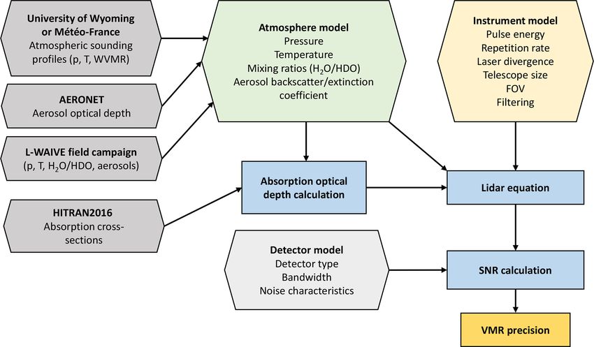
lines at 5044.2277 cm−1 (1982.47 nm) and 5040.4937 cm−1 As schematically depicted in Fig. 2, the DIAL simulator
(1983.93 nm), hereafter referred to as HDO options 1 and 2, consists of three sub-models describing atmospheric prop-
respectively, allowing for a sufficiently high absorption over erties, lidar instrument parameters and detector properties.
several kilometers with negligible interference from other Each model will be explained in more detail in the follow-
gas species. Additionally, a second option for H2 O slightly ing paragraphs. The atmosphere model is based on a set of
detuned from the absorption peak at 1982.97 nm will be dis- standard profiles of temperature, pressure and humidity rep-
cussed as a possibility for reducing the temperature sensitiv- resentative of different climate regions along with aerosol op-
https://doi.org/10.5194/amt-14-6675-2021 Atmos. Meas. Tech., 14, 6675–6693, 2021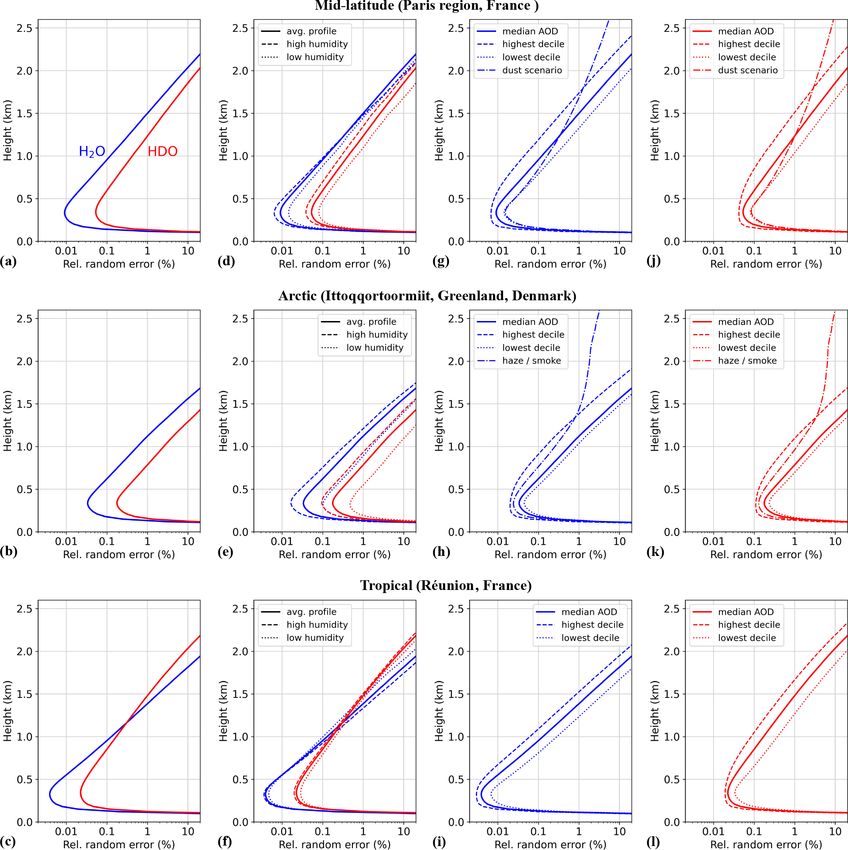
6678                                                   J. Hamperl et al.: Differential absorption lidar for stable water isotopologues

Figure 1. Optical depth over 1 km for H2 16 O (H2 O) and HD16 O (HDO) with uniform volume mixing ratios of 8400 and 2.6 ppmv, respec-
tively (relative humidity of 50 % at 15 ◦ C). (a) Spectral overview between 1 and 3 µm. (b) Close-up window for wavelengths around 2 µm
with decreasing HDO absorption towards 2.05 µm. (c) Spectral range of interest for simultaneous H2 O and HDO sounding. The dashed
black line represents the total optical depth of other species (CO2 , CH4 , N2 O) with their typical atmospheric concentrations. Vertical black
lines indicate the positions of possible off-line wavelengths. On-line wavelengths are indicated for H2 O (vertical blue line for option 1 at
1982.93 nm, dashed blue line for option 2 at 1982.97 nm) and HDO (vertical red line for option 1 at 1982.47 nm, dashed red line for option 2
at 1983.93 nm). Spectra calculations are based on the HITRAN2016 database assuming a temperature of 15 ◦ C and an atmospheric pressure
of 1013.25 hPa.

Table 1. Spectroscopic parameters for selected absorption lines.

                                                          ν                λ                 S               E 00         γair       nair
                       H2 16 O (1)                   5043.0476        1982.928       2.17 × 10⁻²⁴          920.21       0.0367       0.49
                       HD16 O (1)                    5044.2277        1982.464       1.17 × 10⁻²⁴           91.33       0.1036       0.71
                       HD16 O (2)                    5040.4937        1983.933       9.38 × 10⁻²⁵          116.46       0.1003       0.71
                       H2 16 O at HD16 O (1)         5044.2300        1982.463       2.29 × 10⁻²⁵         2756.42       0.0456       0.37

                     ν (cm−1 ): wavenumber; λ (nm): vacuum wavelength; S (cm−1 (molec. cm−2 )−1 ): line intensity at 296 K; E 00 (cm−1 ):
                     lower-state energy; γair (cm−1 atm−1 ): air-broadened Lorentzian half width at half maximum (HWHM) at 1 atm and 296 K;
                     nair : temperature exponent for γair .

tical depth data of the AERONET database (https://aeronet.                          ical approach based on an error propagation calculation to
gsfc.nasa.gov/, last access: 2 October 2021). Those data are                        estimate the random error in the measured isotopic mixing
exploited to calculate the atmospheric transmission using                           ratios and thus the uncertainty in the δD retrieval obtained
absorption cross-sections computed with the HITRAN2016                              with the simulated instrumental parameters.
spectroscopic database (Gordon et al., 2017). Together with                            Starting from the lidar equation (Collis and Russell, 1976),
the model describing the lidar instrument, the calculated                           the calculated received power as a function of distance r is
transmission data are used to feed the lidar equation in or-                        written as
der to calculate the received power at each selected on-line                                      A             c 2
and off-line wavelength. In a subsequent step, noise contri-                        Pr (r) = Tr     2
                                                                                                      βπ (r)O(r) Tatm (r)Ep ,                  (2)
                                                                                                  r             2
butions arising from the detection unit are taken into account
to estimate the signal-to-noise ratio. Then, we use an analyt-                      where Tr is the receiver transmission (assumed value of 0.5
                                                                                    for all calculations), A is the effective area of the receiving

Atmos. Meas. Tech., 14, 6675–6693, 2021                                                                   https://doi.org/10.5194/amt-14-6675-2021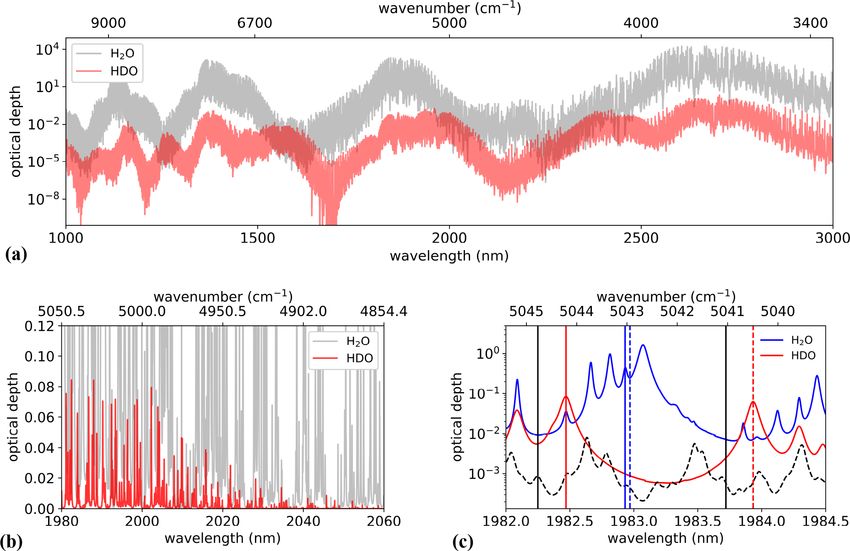
J. Hamperl et al.: Differential absorption lidar for stable water isotopologues                                                     6679

Figure 2. Block diagram of the DIAL simulator. Input models and databases are in hexagons, and principal calculations are indicated by
rectangles. p: pressure; T : temperature; WVMR: water vapor mixing ratio; FOV: telescope field of view. The signal-to-noise ratio (SNR) is
used to calculate the statistical random error (precision) of the volume mixing ratio (VMR) of H2 O/HDO.

telescope, βπ (r) is the backscatter coefficient, O(r) is the          where ρair is the total air number density and σon and σoff are
overlap function between the laser beam and the field of view          the on-line and off-line absorption cross-sections calculated
of the receiving telescope, c is the speed of light, Tatm (r) is       with the HITRAN2016 spectroscopic database assuming a
the one-way atmospheric transmission, and Ep is the laser              Voigt profile representation of the form
pulse energy. The DIAL technique is based on the emission
                                                                                      Z∞
of two wavelengths, one at or close to the peak of an absorp-                     y          exp(−t 2 )
tion line (λon ) and another tuned to the absorption line’s wing       σ (ν) = σ0                           dt,                       (6)
                                                                                  π        y 2 + (x − t)2
(λoff ).                                                                              −∞
   Provided that the two laser pulses are emitted sufficiently         with
close in wavelength and in time for the atmospheric aerosol
                                                                            S ln 2 1/2

content to be equivalent, they experience the same backscat-
                                                                       σ0 =               ,
tering along the line of sight, and the differential optical               γD π
depth 1τ as the difference in on- and off-line optical depth              γ
at a measurement range r can be retrieved by                           y=    (ln 2)1/2 ,
                                                                          γD
                                                                          ν − ν0
                                                                                 (ln 2)1/2 ,

           1      Poff (r)                                             x=
1τ (r) = ln                  ,                               (3)            γD
           2      Pon (r)
                                                                       where S is the line strength, γD is the Doppler width, γ is
with Pon and Poff as the backscattered power signals for λon           the pressure-broadened linewidth and ν0 is the line center
and λoff , respectively. Using the optical depth measurement,          position. The temperature T dependence of the line strength
the gas concentration can be retrieved at a remote range r             is determined by the energy of the lower molecular state E 00
within a range cell 1r = r2 −r1 . Assuming 1r is sufficiently          according to
small, the water vapor content expressed as the volume mix-                     3/2       00
ing ratio, which is assumed as constant within 1r, can then                     T0           E hc 1        1
                                                                       S = S0          exp              −       ,               (7)
be derived by                                                                    T             k     T0 T
                     1τ (r2 ) − 1τ (r1 )                               where T0 is the reference temperature, k is the Boltzmann
XH2 O (r1 → r2 ) =    R r2               ,                     (4)     constant and c is the speed of light.
                        r1 WF(r)dr
                                                                          Equation (3) is valid for the detection of the main isotopo-
with WF(r) representing a weighting function defined as                logue H2 O. For HDO however, the presence of H2 O absorp-
                                                                       tion at the on-line wavelength of HDO (see Fig. 1c) necessi-
WF(r) = (σon (r) − σoff (r)) ρair (r),                         (5)     tates an additional consideration of that bias for the inversion.

https://doi.org/10.5194/amt-14-6675-2021                                                   Atmos. Meas. Tech., 14, 6675–6693, 2021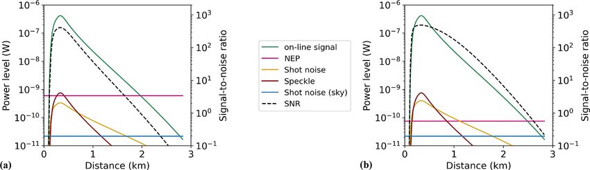
6680                                                          J. Hamperl et al.: Differential absorption lidar for stable water isotopologues

Taking this into account, Eq. (3) changes to                                       determined by an aperture in the telescope’s focal plane. For
                                                                                 better comparability, we assume the same aperture diameter
              1     Poff (r)                                                       of 1.2 mm for both the PIN photodiode and the APD. Given
1τHDO (r) = ln                 − 1τH2 O (r),                                 (8)
              2     Pon (r)                                                        the small active area of the APD, imaging of the field of view
                                                                                   on the detector might, however, prove extremely challenging
where 1τH2 O represents the H2 O differential optical depth                        in practice. The measurement bandwidth of the DIAL sys-
at the HDO on-line wavelength λHDO , which can be calcu-                           tem is effectively determined by an electronic low-pass filter
lated with the knowledge of the volume mixing ratio XH2 O                          in the detection chain. In the simulation we use a bandwidth
measured at λH2 O .                                                                setting of 1 MHz corresponding to a spatial resolution of the
   To obtain an analytical expression for the random error in                      retrieved isotopologue concentrations of 150 m. For all our
the concentration measurement, an error propagation calcu-                         calculations we assume signal averaging over an integration
lation can be applied to Eqs. (3) and (4) assuming that the                        time of 10 min (45 000 laser shots for the on- and off-line
range cell interval 1r is sufficiently small and that the range                    wavelength).
cell resolution of the receiver is sufficiently high to consider                      In order to quantify the measurement uncertainty in the re-
1τ (r1 ) and 1τ (r2 ) uncorrelated. The absolute uncertainty in                    trieved isotope mixing ratios, random and systematic sources
the volume mixing ratio X expressed as the standard devia-                         of errors are taken into account. Random errors in measur-
tion σ (X) can be calculated from the signal-to-noise ratios                       ing the differential optical depth, and thus the species mix-
of the on- and off-line power signals as follows:                                  ing ratio, are related to different noise contributions arising
                                                   !1/2                            from the detection setups. For a single return-signal pulse,
            1f            1                1                                       the associated noise power Pn consists of a constant detec-
σ (X) = √            +                                    ,                  (9)
         2WF c SNR2on SNR2off                                                      tor and amplifier noise expressed as noise-equivalent power
                                                                                   NEP, shot noise due to background radiation Psky , shot noise
where 1f is the measurement bandwidth which is the same                            dependent on the pulse power P (λ) and speckle noise Psp (λ):
for the on- and off-line pulses since they are measured se-                               q
quentially by the same detector. Finally, with both uncertain-                     Pn =       (NEP2 + 2 · e · [Psky + P (λ)] · F /R) · 1f + Psp
                                                                                                                                              2 (λ), (11)

ties in the volume mixing ratios XH2 O and XHDO known, an
estimation of the uncertainty in δD is obtained by applying                        where e is the elementary charge, F the excess noise factor
an error propagation calculation to Eq. (1) in order to obtain                     (in the case of the APD), R the detector responsivity (de-
the expected uncertainty expressed as variance:                                    pending on quantum efficiency in the case of the APD) and
                                                                                   1f the measurement bandwidth. The NEP of 600 fW Hz−1/2
                    (                2                       2 )1/2            for configuration i featuring the InGaAs PIN photodiode is a
                         σ (XH2 O )          σ (XHDO )
σ (δD) = (δD + 1)                          +                              . (10)   conservative estimate by calculations based on the specifica-
                           X H2 O              XHDO
                                                                                   tions of the photodiode and amplifier manufacturer (G12182-
2.3    Instrument and detector model                                               003K InGaAs PIN photodiode from Hamamatsu combined
                                                                                   with a gain-adjustable DHPCA-100 current amplifier from
In order to estimate the feasibility of a DIAL measure-                            FEMTO). The background power Psky depends on the back-
ment, calculations were performed for the transmitter and re-                      ground irradiance Ssky and the receiver geometry according
ceiver parameters summarized in Table 2. The emitter of the                        to
DIAL system will be based on a generic optical parametric                                  π                      2
                                                                                   Psky = · Ssky · 1λf · Aeff · θFOV   ,                   (12)
oscillator–optical parametric amplifier (OPO–OPA) architec-                                 4
ture like the one developed in Barrientos Barria et al. (2014).
                                                                                   where 1λf , Aeff and θFOV are the optical filter band-
The combination of a doubly resonant nested-cavity OPO
                                                                                   width, effective receiver telescope area and field of view
(NesCOPO) and an OPA pumped by a 1064 nm Nd:YAG
                                                                                   angle, respectively. A constant background irradiance of
commercial laser with a 150 Hz repetition rate allows for
                                                                                   1 W m−2 µm−1 sr−1 and an optical filter bandwidth of 50 nm
single-frequency, high-energy pulses with adequate tunabil-
                                                                                   are used for all calculations. Assuming Gaussian beam char-
ity. From this system we expect an extracted signal energy of
                                                                                   acteristics, the speckle-related noise power is approximately
up to 20 mJ at 1983 nm. For a more conservative estimate, we
                                                                                   given by Ehret et al. (2008):
will also consider a lower-limit pulse energy of 10 mJ for our
simulations. The receiver part consists of a Cassegrain-type                                           √
                                                                                                  λ · 2 1f · τc
telescope with a primary mirror of 40 cm in diameter. For                          Psp = P (λ) ·                  ,                         (13)
                                                                                                  π · Rtel · θFOV
the detection part, calculations were performed in a direct-
detection setup for (i) a commercial InGaAs PIN photodi-                           where Rtel denotes the telescope radius and τc the coherence
ode and (ii) a HgCdTe avalanche photodiode (APD) specifi-                          time of the laser pulse corresponding to the pulse duration for
cally developed for DIAL applications in the 2 µm range, pre-                      a Fourier-transform-limited pulse. Finally, the overall time-
sented in Gibert et al. (2018). The telescope field of view is                     averaged signal-to-noise ratio is given as the ratio of received

Atmos. Meas. Tech., 14, 6675–6693, 2021                                                                 https://doi.org/10.5194/amt-14-6675-2021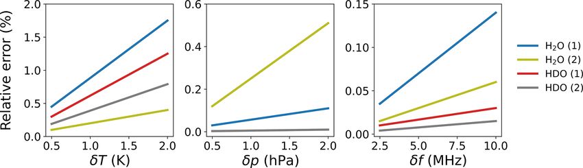
J. Hamperl et al.: Differential absorption lidar for stable water isotopologues                                                6681

Table 2. DIAL instrument parameters.

                       Transmitter                                            Receiver
              Energy            10–20 mJ                             (i)                        (ii)
              Pulse duration    10 ns          Telescope aperture    40 cm                      40 cm
              Repetition rate   150 Hz         Detector type         InGaAs PIN                 HgCdTe APD
              λon H2 16 O (1)   1982.93 nm     Detector diameter     300 µm                     180 µm
              λon H2 16 O (2)   1982.97 nm     Field of view (FOV)   630 µrad                   630 µrad
              λon HD16 O (1)    1982.47 nm     NEP                   600 fW Hz−1/2              75 fW Hz−1/2
              λon HD16 O (2)    1983.93 nm     Bandwidth             1 MHz                      1 MHz
              Divergence        270 µrad                             Responsivity: 1.2 A W−1    Quantum efficiency: 0.8
                                                                                                Excess noise factor: 1.2

power from Eq. (2) and total noise power from Eq. (11) mul-          the right column of Fig. 3g–i. Median values of the AOD are
tiplied by the square root of the number of laser shots N:           used for the baseline model. The lowest (AOD10 ) and highest
         Pr √                                                        (AOD90 ) decile values serve as input for the sensitivity anal-
SNR =         N.                                         (14)        ysis to model conditions of low and high aerosol charge, re-
         Pn
                                                                     spectively. As a next step, vertical profiles of aerosol extinc-
2.4   Atmosphere model                                               tion are constructed by making basic assumptions about their
                                                                     shape and constraining their values by the extrapolated AOD.
We constructed different atmospheric models for mid-                 In our baseline model, the vertical distribution of aerosols is
latitude, arctic and tropical locations to study the sensitivity     represented by an altitude-dependent Gaussian profile of the
of the DIAL measurement to environmental factors. The at-            extinction coefficient with varying half width depending on
mosphere model consists of vertical profiles of pressure, tem-       the location (Fig. 3d–f). This type of profile roughly corre-
perature and humidity (see Appendix A for origin of sound-           sponds to the ESA Aerosol Reference Model of the Atmo-
ing data) which serve as input to calculate altitude-dependent       sphere (ARMA) (ARMA, 1999) which is plotted for each
absorption cross-sections using the HITRAN2016 spectro-              region normalized to the AOD90 -derived extinction profile
scopic database. For the sake of simplicity, HDO mixing ra-          maximum.
tios were obtained from H2 O profiles simply by consider-               However, the distribution of tropospheric aerosols varies
ing their natural abundance of 3.11 × 10⁻⁴ ; i.e., variability in    widely from region to region (Winker et al., 2013). To
terms of the isotopic ratio δD is not assumed in our model.          broadly reflect the different boundary layer characteristics
For each location, a baseline model was constructed by using         for each environment, the extinction profile was adapted
the columns of pressure, temperature and volume mixing ra-           accordingly. In mid-latitude regions, vertical aerosol distri-
tios averaged over the year of 2019. To reflect seasonal varia-      butions vary widely due to regional and seasonal factors
tions in our sensitivity analysis, we use profiles with the low-     (Chazette and Royer, 2017). The planetary boundary layer
est and highest monthly averages of temperature and humid-           (PBL) height can range from a few hundred meters up to
ity (Fig. 3a–c). To complement the atmospheric model, data           3 km (Matthias et al., 2004; Chazette et al., 2017). Assuming
of level 2.0 aerosol optical depth (AOD) from the AERONET            that aerosols are mostly confined to the PBL and that the free
database (https://aeronet.gsfc.nasa.gov/, last access: 2 Oc-         tropospheric contribution to aerosol extinction is weak, the
tober 2021) were used. AERONET sun-photometer prod-                  half-Gaussian-shaped baseline model used for the simula-
ucts are usually available for wavelengths between 340 and           tions gives rise to 85 % of AOD within the first 1.5 km. Since
1640 nm. For extrapolation to the 2 µm spectral region, we           high aerosol loads in the free troposphere due to long-range
used the wavelength dependence of the AOD described by a             dust transport are not uncommon over western Europe (Ans-
power law of the form (Ångström, 1929)                               mann et al., 2003), a dust scenario profile constrained by the
                −α                                                 highest-decile AOD was also investigated. Dust aerosols are
 AOD(λ)           λ
            =            ,                                   (15)    represented by a Gaussian profile above the PBL extending
AOD(λ0 )         λ0
                                                                     well up to a height of 5 km. For this case, aerosol extinction
where AOD(λ) is the optical depth at wavelength λ,                   in the PBL below 1.5 km accounts for half of the total AOD,
AOD(λ0 ) is the optical depth at a reference wavelength and          while dust in the free troposphere accounts for the other half.
α represents the Ångström exponent. The Ångström expo-               At high latitudes, the boundary layer tends to be stable and
nent was obtained by fitting Eq. (15) to the available AOD           extends from a few meters to a few hundred meters above
data in the above-mentioned spectral range in order to ex-           ground. Our baseline Arctic extinction profile thus contains
trapolate further to 1.98 µm. Histograms of the yearly dis-          95 % of the AOD within the first 1.5 km since most aerosols
tribution of the extrapolated AOD at 1.98 µm are shown in

https://doi.org/10.5194/amt-14-6675-2021                                                 Atmos. Meas. Tech., 14, 6675–6693, 2021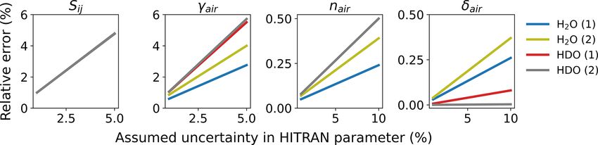
6682                                             J. Hamperl et al.: Differential absorption lidar for stable water isotopologues

Figure 3. Atmosphere models: (a–c) vertical sounding profiles of temperature and the water vapor mixing ratio (WVMR). Grey lines indicate
monthly averages; solid green line is the yearly average of 2019 (baseline profile). Dotted lines indicate profiles of the lowest and highest
monthly temperatures and WVMR; (d–f) model profiles of aerosol extinction coefficient; (g–i) distribution of the aerosol optical depth at
1983 nm for AERONET level 2.0 data of 2019.

Atmos. Meas. Tech., 14, 6675–6693, 2021                                                    https://doi.org/10.5194/amt-14-6675-2021
J. Hamperl et al.: Differential absorption lidar for stable water isotopologues 6683
are confined within the first kilometer of the troposphere as kilometer for both detectors and to values around 102 at a
observed by space-borne lidar during long-term studies of the 2 km range for the commercial PIN detector and 103 for the
global aerosol distribution (Di Pierro et al.,2013). The occur- HgCdTe APD.
rence histogram in Fig. 3h shows very low values of AOD for The expected relative random errors in the mixing ratios of
most of the time in the available photometer products from H2 O and HDO are shown separately for each detector in the
February to September. The long-tailed wing of the asym- upper and lower panels of Fig. 5. We examined two scenarios
metric distribution towards higher values can be explained with different laser pulse energies of 10 and 20 mJ, a mea-
by seasonally occurring episodes of arctic haze due to anthro- surement bandwidth of 1 MHz (150 m range cell resolution),
pogenic aerosols transported from mid-latitude regions (win- and an integrating time of 10 min for a repetition rate (on–off
ter to spring) and boreal forest fire smoke during the summer rate) of 150 Hz. The simulation based on the 20 mJ configu-
season (Tomasi et al., 2015; Chazette et al., 2018). ration gives an estimation of the best-case precision limit of
Similarly to the dust scenario for the mid-latitude model, the DIAL system. The second configuration with 10 mJ pulse
haze and smoke events are modeled by an additional Gaus- energy can be understood as a lower limit on the precision of
sian profile in the free troposphere constrained by the measuring mixing ratios of H2 O and HDO and finally δD.
highest-decile AOD. Extinction profiles representing the As shown in Fig. 5, a relative random error of well un-
tropical environment of the island of Réunion, where sea salt der 1 % in the mixing ratio of both H2 O and HDO can be
aerosols can be assumed to be the dominant aerosol species, achieved within the first kilometer for both detectors and
are chosen such that 90 % of the AOD is attributed to the first 20 mJ pulse energy. The degraded precision for measuring
1.5 km. HDO is due to its lower differential absorption compared to
Vertical profiles of the aerosol backscatter coefficient were H2 O. The slight difference in optical depth for the two HDO
calculated assuming, for the sake of simplicity, a constant options leads only to a small loss in precision for wavelength
extinction-to-backscatter ratio (lidar ratio) of 40 sr through- option 2. For the low-noise APD shown in the bottom panel
out all sets of extinction profiles. of Fig. 5, the simulations show that even for the conservative
assumption of 10 mJ pulse energy, the relative error stays be-
low 1 % for both H2 O and HDO over a range of 1.5 km corre-
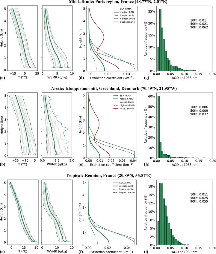
3 Simulation results and discussion sponding to typical heights of the planetary boundary layer.
H2 O uncertainties were calculated for sounding at the peak
3.1 Instrument random error of the absorption line (option 1). The simulation results also
reveal a sharp rise in the random uncertainty towards longer
This section aims to quantify the random error in the mixing distances which is attributed to the drastic decline in aerosol
ratio measurement depending on instrument settings such as backscatter in the free troposphere in our model. The sharp
laser pulse energy and the type of detector employed. All cal- fall of the random error within the first 200–300 m is due
culations are based on the mid-latitude baseline atmosphere to the increasing overlap between the laser beam and tele-
model assuming vertical sounding of the lower troposphere scope field of view imaged onto the detector described by
with aerosols confined to the lowest 2 km. Considering a sim- the overlap function O(r) in Eq. (2). This overlap term is
ple calculation of random errors, we will discuss their im- zero directly in front of the lidar instrument and reaches unity
plications for the precision of the measurement of range- after around 450 m for the here-described configuration. It
resolved δD profiles. Given the instrument parameters pre- should be noted that for the range zone of non-uniform over-
sented in Table 2, the dominant noise contributions are esti- lap, slight differences between the on- and off-line overlap,
mated, which are shown for a single on-line pulse in Fig. 4 for example due to laser beam pointing, can induce signifi-
for both detector configurations. cant systematic errors. From a practical point of view, the ex-
As expected, the electronic noise level is significantly re- pected lowest instrument range is thus closer to 0.5 km than
duced by roughly 1 order of magnitude for the HgCdTe APD the distance suggested by the location of the random error
combined with a transimpedance amplifier due to a low com- minima around 250 m.
bined NEP of 75 fW Hz−1/2 compared to 600 fW Hz−1/2 for Figure 5c and f show the expected precision in δD which
the amplifier of the InGaAs PIN detector. In fact, shot noise depends on the relative random errors in the volume mix-
and speckle are predominant for the APD for the first kilo- ing ratios for H2 O and HDO (see Eq. 9). For the commercial
meter of range, whereas the electronic noise of the tran- InGaAs PIN photodiode we find for the best-case configura-
simpedance amplifier is the predominant contribution over tion (20 mJ pulse energy, 1 MHz bandwidth) that the abso-
the entire range for the commercial PIN detector. Signal-to- lute value of uncertainty in δD is below 3 ‰ within a range
noise ratios of up to 102 are obtained for a single measure- of 1 km. The 10 mJ configuration also allows for measure-
ment pulse within the first kilometer. Integrating over 45 000 ment of δD, although with deteriorated absolute precision of
laser shots (equivalent to 10 min averaging time if on- and up to 10 ‰ within the first kilometer. For greater ranges, the
one off-line wavelengths are addressed sequentially) would precision levels decline rapidly and are not sufficient to re-
increase the signal-to-noise ratios to over 104 in the first solve variations in δD on the order of a few tens of per mil.
https://doi.org/10.5194/amt-14-6675-2021 Atmos. Meas. Tech., 14, 6675–6693, 20216684 J. Hamperl et al.: Differential absorption lidar for stable water isotopologues
Figure 4. Received power according to Eq. (2) (solid green line) and power-equivalent levels of major noise contributions related to the H2 O
on-line signal for a single 20 mJ pulse and resulting signal-to-noise ratio (SNR, dashed black line, right vertical axis) as function of lidar
range: (a) InGaAs PIN detector, (b) low-noise HgCdTe APD.
Figure 5. Expected relative random error in the volume mixing ratio of H2 O and HDO for different pulse energies (solid lines: 20 mJ; dashed
lines: 10 mJ) and detectors: (a–b) InGaAs PIN detector, (d–e) HgCdTe APD. (c, f) Corresponding absolute uncertainty (standard deviation)
in δD as a function of distance from the lidar instrument. A detection bandwidth of 1 MHz is assumed, and signal averaging time is 10 min.
The use of a HgCdTe APD detector can overcome this limi- eter under investigation. Simulation results are summarized
tation where calculations indicate that an absolute precision in Fig. 6 for targeting H2 O at 1982.93 nm (blue) and HDO
level better than 10 ‰ within a range of close to 2 km can be at 1983.93 nm (red). Here again, we consider a measurement
achievable with 20 mJ laser energy. bandwidth of 1 MHz (150 m range cell resolution) and an in-
tegrating time of 10 min for a repetition rate of 150 Hz. All
3.2 Sensitivity to atmospheric variability calculations have been performed with the InGaAs PIN de-
tector and assuming a laser pulse energy of 20 mJ.
The sensitivity of the DIAL instrument to the variability in Starting with temperature, no effect on the measurement
temperature, humidity and aerosol load was investigated for random error was found when simulating under conditions
the mid-latitude, arctic and tropical atmosphere models. In of lower and higher temperature compared to the average
the following analysis, the relative random error (precision) atmospheric columns. Comparing the three baseline models
is used to compare the influence of each atmospheric param- of mid-latitude, tropical and arctic environments, the perfor-
Atmos. Meas. Tech., 14, 6675–6693, 2021 https://doi.org/10.5194/amt-14-6675-2021J. Hamperl et al.: Differential absorption lidar for stable water isotopologues 6685 Figure 6. Sensitivity with respect to variability in atmospheric parameters: resulting statistical uncertainty for range-resolved DIAL mea- surement of H2 O (blue, option 1 at 1982.93 nm) and HDO (red, option 2 at 1983.93 nm). Simulation parameters: 20 mJ pulse energy, 1 MHz bandwidth, 10 min integration time, InGaAs PIN detector. (a–c) Reference model based on average columns of pressure, temperature and humidity. Aerosol baseline profile using median AOD assumed. (d–f) Sensitivity to water vapor variability. (g–i) Sensitivity to different aerosol profiles (H2 O). (j–l) Sensitivity to different aerosol profiles (HDO). mance simulations find that the highest-precision measure- faster than for HDO with increasing range due to strong ments can be achieved under tropical conditions due to high absorption leading to low return signals. On the contrary, humidity levels and favorable aerosol backscattering. Rela- random uncertainties for the arctic environment are almost tive random errors lower than 0.1 % for H2 O are achievable 1 order of magnitude higher due to rather dry conditions in within the first kilometer. The precision for H2 O degrades terms of the WVMR and low aerosol content observed at the https://doi.org/10.5194/amt-14-6675-2021 Atmos. Meas. Tech., 14, 6675–6693, 2021
6686                                          J. Hamperl et al.: Differential absorption lidar for stable water isotopologues

eastern Greenland AERONET station of Ittoqqortoormiit. A           sorption peak (option 2) results in a noticeable reduction in
high sensitivity to seasonal variability in the humidity profile   the temperature error. However, this comes at the expense
was observed for the arctic model, whereas variations in hu-       of increased pressure error and a lower signal-to-noise ratio
midity in the tropics throughout the year are small and thus       and thus increased random error for unchanged laser energy,
only slightly affect the expected measurement precision. The       integration time and bandwidth. Considering the mentioned
simulations also clearly show the influence of aerosols on         systematic error contributions, option 2 for H2 O proves to be
the performance of DIAL measurements. For all three lo-            the preferred wavelength choice with the intention of reduc-
cations, the precision gain between the low-charge (lowest-        ing the systematic error, especially if the temperature profile
decile AOD) and high-charge (highest-decile AOD) aerosol           along the line of sight is not known with an accuracy better
model is roughly 1 order of magnitude. The presence of free        than ±0.5 K.
tropospheric aerosols, for example due to long-range dust             For the case of instrument-related errors, we estimated
transport in the mid-latitudes and arctic haze or boreal forest    systematic errors arising from the laser wavelength locking
fire smoke in the Arctic, leads to significant improvements in     control and spectral quality of the laser beam. To estimate the
the precision at altitudes beyond the atmospheric boundary         sensitivity to laser line stability, laser frequency deviations
layer.                                                             δf ranging from 2.5 to 10 MHz were simulated. The chosen
                                                                   values correspond to wavelength stabilities reliably achiev-
3.3    Systematic errors                                           able over several minutes with our envisioned OPO–OPA ap-
                                                                   proach coupled to a commercial wavemeter, which can suffer
Systematic errors are associated with an uncertainty in the        thermal drifts of a few megahertz over several tens of min-
knowledge of atmospheric-, spectroscopic- and instrument-          utes. The relative wavelength error was calculated according
related parameters when obtaining the VMR from the mea-            to Eq. (16) by introducing a wavelength detuning δf to the
sured differential optical depth according to Eq. (4). Ex-         on- and off-line wavelengths. Due to the narrower absorption
pressed in a general form, errors were estimated by calcu-         line of H2 O at 1982.93 nm, we find that such wavelength de-
lating the VMR retrieval sensitivity to a deviation δY from a      tuning results in a greater error compared to the spectrally
reference parameter Y :                                            larger HDO line. Option 2 for H2 O measurement reduces the

            |X(Y ) − X(Y ± δY )|
                                                                  wavelength error. The systematic error due to the finite laser
εs = max                            .                     (16)     linewidth was estimated numerically by substituting the ab-
                    X(Y )
                                                                   sorption cross-sections of Eq. (5) by the effective absorption
For the case of atmospheric systematic errors, the reference       cross-sections defined as
parameter Y used for the VMR retrieval stands for either the               R
                                                                             L(ν, r) · σ (ν, r) · dν
vertical pressure or the temperature profile of the baseline       σeff =      R                     ,                        (17)
                                                                                 L(ν, r) · dν
atmospheric model. The systematic error due to an uncer-
tainty in the knowledge of the temperature profile was calcu-      where L represents the spectral intensity distribution of
lated for temperature deviations δT from the reference pro-        the laser transmitter and ν denotes the wavenumber. The
file ranging from ±0.5 to ±2 K. This range of accuracy can         laser spectral distribution L is assumed to be an altitude-
be obtained by in situ sensors or an additional lidar instru-      independent Gaussian function with a full width at half max-
ment for the temperature profile which is necessary to calcu-      imum of 50 MHz, which correlates roughly to the 10 ns pulse
late the temperature-dependent absorption cross-sections for       duration assuming transform-limited pulses. For comparison,
the concentration retrieval. As shown in Fig. 7, this kind of      the air-broadened Lorentzian widths of the absorption lines
error can lead to a significant contribution to the error bud-     under standard atmospheric conditions are on the order of a
get. The analysis shows that sounding H2 O at the absorption       few gigahertz. The calculated relative error is on the order
peak is especially sensitive to temperature uncertainties and      of 0.1 % for the narrowest (thus most critical) H2 O line at
that a measurement with the on-line wavelength shifted off         1982.93 nm.
the absorption peak (H2 O option 2) significantly reduces this        Another systematic error arises for sounding HDO at
bias. Table 3 gives an overview of the calculated biases com-      1982.47 nm (option 2) from the insufficient knowledge of
paring the three different atmospheric models. Note the sig-       the optical depth due to the non-negligible H2 O absorption
nificant temperature bias for HDO option 1 in regions with         feature. Assuming a relative uncertainty of 2 % in the VMR
high water vapor content due to the highly temperature sensi-      profile of H2 O, which is a conservative estimate for the com-
tive H2 O interference line. Similarly, a pressure deviation δp    bined systematic error in the H2 O measurement due to tem-
ranging from 0.5 to 2 hPa was used to estimate the error due       perature, pressure and wavelength uncertainty, calculations
to an uncertainty in the pressure profile. In this case, H2 O      reveal relative errors in the VMR retrieval varying between
wavelength option 2 is more sensitive to such an uncertainty.      0.28 % for the arctic model and 0.83 % for the tropical model.
The resulting bias in the measurement of HDO is found to           Considering this additional bias and the highly temperature
be negligible. Note the difference between the two options         sensitive H2 O interference line for HDO option 1, option 2
for probing H2 O. Shifting the on-line wavelength off the ab-      should be the preferred wavelength option for HDO in any

Atmos. Meas. Tech., 14, 6675–6693, 2021                                             https://doi.org/10.5194/amt-14-6675-2021
J. Hamperl et al.: Differential absorption lidar for stable water isotopologues 6687
Figure 7. Maximal relative error in the VMR retrieval (over 3 km range, mid-latitude baseline) due to uncertainties in the profiles of tem-
perature (δT ) and atmospheric pressure (δp) as well as transmitter on- and off-line wavelength (δf ). The parenthetical numbers (1) and (2)
stand for the two possible on-line wavelength options for measuring H2 O.
Table 3. Systematic errors for mid-latitude, arctic and tropical atmospheric models (maximal error over 3 km range). The parenthetical
numbers (1) and (2) denote the two wavelength options for H2 O and HDO measurements.
Parameter Assumed Maximal relative error εs
uncertaintya (%)
Mid-latitude Arctic Tropic
H2 O H2 O HDO HDO H2 O H2 O HDO HDO H2 O H2 O HDO HDO
(1) (2) (1) (2) (1) (2) (1) (2) (1) (2) (1) (2)
Temperature ±1 K 0.85 0.21 0.61 0.39 0.95 0.27 0.19 0.40 0.79 0.15 1.12 0.37
Pressure ±1 hPa 0.08 0.27 < 0.01 < 0.01 0.06 0.26 < 0.01 < 0.01 0.05 0.25 < 0.01 < 0.01
On–off wavelength 5 MHz 0.07 0.03 0.02 < 0.01 0.07 0.04 0.02 < 0.01 0.07 0.03 0.03 < 0.01
VMR of H2 O bias 2 %b – – 0.52 – – – 0.28 – – – 0.83 –
HITRAN2016 parameters
Line intensity 1% 1.00 1.00 1.01 1.00 1.00 1.00 1.01 0.99 1.00 1.00 1.01 0.99
Air-broadened width γair 1% 0.60 0.86 1.05 1.06 0.59 0.87 1.07 1.06 0.57 0.83 1.05 1.05
T exponent of γair 5% 0.14 0.20 0.33 0.33 0.21 0.31 0.49 0.49 0.07 0.1 0.16 0.16
Pressure shift 5% 0.15 0.19 0.03 < 0.01 0.15 0.16 0.04 < 0.01 0.13 0.21 0.03 < 0.01
Combined (geometric sum) 1.48 1.39 1.69 1.54 1.53 1.42 1.59 1.58 1.41 1.35 2.02 1.50
a Relative uncertainty if stated is in percent. b Conservative estimate of combined systematic error for H O measurement.
2
case. It should be noted that even for the measurement of form of an error budget for each of the three atmospheric
H2 O, an interference contribution due to higher HDO absorp- models is given in Table 3.
tion at the off-line wavelength leads to a bias. However, this
error is relatively small compared to other systematic errors 3.4 Precision estimate applied to field campaign data
and the achievable random error.
Finally, systematic errors in the VMR retrieval due to un- In order to complete our previous numerical studies and re-
certainties related to spectroscopic parameters were analyzed late to more realistic atmospheric conditions, we present here
by introducing deviations between 1 % to 5 % into the HI- the results of performance calculations initialized with ob-
TRAN2016 parameters of line intensity and air-broadened servations obtained during the L-WAIVE (Lacustrine-Water
width and deviations of 1 % to 10 % to the temperature- vApor Isotope inVentory Experiment) field campaign at
dependent width coefficient and the pressure shift parameter. the Annecy lake in the French Alpine region (Chazette et
The resulting systematic errors are shown in Fig. 8 for each al., 2021). This experiment was specifically carried out in
parameter. Uncertainties in parameters of line intensity and order to obtain reference profiles that can be used to simu-
air-broadened width largely contribute to the error budget, late the WaVIL lidar vertical profiles. Hence, the data include
highlighting the importance of having precise knowledge of vertical profiles of pressure and temperature as well as ver-
these quantities. It should be noted that the assumed uncer- tical profiles of H2 O and HDO isotopologue concentrations
tainties have a rather demonstrative character as their precise which were obtained by an ultra-light aircraft equipped with
quantification is still the subject of ongoing spectroscopic an in situ cavity-ring-down-spectrometer (CRDS) isotope an-
studies. A summary of the presented systematic errors in the alyzer. As aerosols were present above the planetary bound-
ary layer on 14 June 2019, we chose data acquired from that
https://doi.org/10.5194/amt-14-6675-2021 Atmos. Meas. Tech., 14, 6675–6693, 20216688 J. Hamperl et al.: Differential absorption lidar for stable water isotopologues
Figure 8. Maximal relative error in the VMR retrieval (over 3 km range, mid-latitude baseline) due to uncertainties in HITRAN parameters.
Sij : line intensity; γair : air-broadened half width; nair : coefficient of the temperature dependence of γair ; δair : pressure shift.
day, ranging up to an elevation of 2.3 km. To simulate atmo- should be noted that the presented profiles represent a rather
spheric conditions during the measurement campaign as re- favorable case since the aerosol backscatter coefficient in-
alistically as possible, we used aerosol extinction data from creases with altitude (due to the presence of an elevated dust
the lidar WALI (Weather and Aerosol Lidar) (Chazette et layer) which is contrary to the baseline atmospheric models
al., 2014) operated during the L-WAIVE campaign on the described in the previous numerical analysis. These simula-
same day (see Fig. 9a). The backscatter coefficient was esti- tions incorporating observed H2 O and HDO profiles clearly
mated with a lidar ratio of 50 sr and extrapolated to a wave- show the potential of a ground-based DIAL instrument to
length of 2 µm using the Ångström exponent derived from measure isotopic mixing ratios with a high spatio-temporal
sun-photometer measurements. For the purpose of our sim- resolution in the lower troposphere.
ulation study, we do not take into account any measurement
uncertainties in the described profiles. Figure 9b and c show
the in situ-measured δD profile from the field campaign and 4 Conclusions
the hypothetical precision of δD as the shaded area depend-
ing on detector characteristics and laser energy if that same Probing the troposphere for water isotopologues with a high
profile was measured with the here-presented DIAL system spatio-temporal resolution is of great interest to studying pro-
(precision estimate based on wavelength option 1 for H2 O cesses related to weather and climate, atmospheric radiation,
and option 2 for HDO). and the hydrological cycle. In this context, the Water Vapor
For the commercial InGaAs PIN photodiode, the simula- Isotope Lidar (WaVIL), which will measure H2 O and HDO
tions show for the optimum case of 20 mJ laser energy that based on the differential absorption technique, is under de-
the uncertainty related to noise is sufficiently low for the velopment. The spectral window between 1982–1984 nm has
characteristic variations in the experimentally obtained δD been identified to perform such measurements. The selected
profile to be fully resolved with the proposed DIAL sys- absorption lines of H2 O and HDO have a sufficiently high
tem. In terms of absolute precision, which is visualized as line strength to probe the lower 1.5 km of the atmosphere
the width of the shaded error band around the in situ pro- with better than 1 % relative error in the tropics and mid-
file, δD could be determined with a precision better than 5 ‰ latitude regions with high water vapor concentrations. The
within the first 1.5 km and better than 10 ‰ at a range height selected absorption lines are temperature sensitive, requiring
of 2 km. A setup with 10 mJ would deliver an absolute preci- accurate knowledge of the temperature profile along the line
sion close to 20 ‰ at that height. The expected precisions are of sight for the concentration retrieval. Such a profile would
on the order of or better than the columnar measurements ob- have to be provided by auxiliary measurements, for example
tained with other remote sensing techniques deployed from by using a Raman lidar.
the ground (between 5 ‰ and 35 ‰ for a Fourier transform We performed a sensitivity analysis and an error budget
infrared spectrometer and the Total Carbon Column Observ- for this system taking instrument-specific and environmen-
ing Network) or from space (∼ 40 ‰ for the Tropospheric tal parameters into account. The numerical analysis included
Emission Spectrometer and the Infrared Atmospheric Sound- models of mid-latitude, polar and tropical environments with
ing Interferometer; see Table 1 of Risi et al., 2012) but with realistic aerosol loads derived from the AERONET database
a much greater resolution on the vertical. On the other hand, extrapolated to the 2 µm spectral region. We showed that the
the expected precision is roughly 2 to 4 times lower than for retrieval of H2 O and HDO mixing ratios is possible with rel-
in situ airborne CRDS measurements with a similar vertical ative random errors better than 1 % within the atmospheric
resolution (see Table 3 of Sodemann et al., 2017). Simula- boundary layer (< 2 km) in mid-latitude and tropical condi-
tions performed with the HgCdTe APD indicate extremely tions, the latter giving rise to the highest precision due to fa-
promising precision levels over the entire range of under 3 ‰ vorable differential absorption. Based on these precisions of
and 5 ‰ (in absolute terms) for 20 and 10 mJ, respectively. It the mixing ratio measurements, the isotopic abundance ex-
pressed in δD notation can be derived with a precision nec-
Atmos. Meas. Tech., 14, 6675–6693, 2021 https://doi.org/10.5194/amt-14-6675-2021You can also read