Distribution of planktonic biogenic carbonate organisms in the Southern Ocean south of Australia: a baseline for ocean acidification impact assessment
←
→
Page content transcription
If your browser does not render page correctly, please read the page content below
Biogeosciences, 15, 31–49, 2018
https://doi.org/10.5194/bg-15-31-2018
© Author(s) 2018. This work is distributed under
the Creative Commons Attribution 3.0 License.

Distribution of planktonic biogenic carbonate organisms in the
Southern Ocean south of Australia: a baseline for ocean
acidification impact assessment
Thomas W. Trull1,2,3 , Abraham Passmore1,2 , Diana M. Davies1,2 , Tim Smit4 , Kate Berry1,2 , and Bronte Tilbrook1,2
1 Climate   Science Centre, Oceans and Atmosphere, Commonwealth Scientific and Industrial Research Organisation,
Hobart, 7001, Australia
2 Antarctic Climate and Ecosystems Cooperative Research Centre, Hobart, 7001, Australia
3 Institute of Marine and Antarctic Studies, University of Tasmania, Hobart, 7001, Australia
4 Utrecht University, Faculty of Geosciences, Utrecht, 3508, the Netherlands

Correspondence: Thomas W. Trull (tom.trull@csiro.au)

Received: 1 June 2017 – Discussion started: 12 June 2017
Revised: 5 November 2017 – Accepted: 8 November 2017 – Published: 3 January 2018

Abstract. The Southern Ocean provides a vital service by          associated POC, representing less than 1 % of total POC
absorbing about one-sixth of humankind’s annual emis-             in Antarctic waters and less than 10 % in subantarctic wa-
sions of CO2 . This comes with a cost – an increase in            ters. NASA satellite ocean-colour-based PIC estimates were
ocean acidity that is expected to have negative impacts           in reasonable agreement with the shipboard results in sub-
on ocean ecosystems. The reduced ability of phytoplank-           antarctic waters but greatly overestimated PIC in Antarc-
ton and zooplankton to precipitate carbonate shells is a          tic waters. Contrastingly, the NASA Ocean Biogeochemical
clearly identified risk. The impact depends on the signif-        Model (NOBM) shows coccolithophores as overly restricted
icance of these organisms in Southern Ocean ecosystems,           to subtropical and northern subantarctic waters. The cause
but there is very little information on their abundance or        of the strong southward decrease in PIC abundance in the
distribution. To quantify their presence, we used coulomet-       Southern Ocean is not yet clear. The poleward decrease in
ric measurement of particulate inorganic carbonate (PIC) on       pH is small, and while calcite saturation decreases strongly
particles filtered from surface seawater into two size frac-      southward, it remains well above saturation (> 2). Nitrate
tions: 50–1000 µm to capture foraminifera (the most impor-        and phosphate variations would predict a poleward increase.
tant biogenic carbonate-forming zooplankton) and 1–50 µm          Temperature and competition with diatoms for limiting iron
to capture coccolithophores (the most important biogenic          appear likely to be important. While the future trajectory of
carbonate-forming phytoplankton). Ancillary measurements          coccolithophore distributions remains uncertain, their current
of biogenic silica (BSi) and particulate organic carbon (POC)     low abundances suggest small impacts on overall Southern
provided context, as estimates of the biomass of diatoms          Ocean pelagic ecology.
(the highest biomass phytoplankton in polar waters) and to-
tal microbial biomass, respectively. Results for nine transects
from Australia to Antarctica in 2008–2015 showed low lev-
els of PIC compared to Northern Hemisphere polar waters.          1   Introduction
Coccolithophores slightly exceeded the biomass of diatoms
in subantarctic waters, but their abundance decreased more        The production of carbonate minerals by planktonic organ-
than 30-fold poleward, while diatom abundances increased,         isms is an important and complex part of the global carbon
so that on a molar basis PIC was only 1 % of BSi in Antarc-       cycle and climate system. On the one hand, carbonate pre-
tic waters. This limited importance of coccolithophores in        cipitation raises the partial pressure of CO2 reducing the up-
the Southern Ocean is further emphasized in terms of their        take of carbon dioxide from the atmosphere into the surface

Published by Copernicus Publications on behalf of the European Geosciences Union.
32                     T. W. Trull et al.: Distribution of planktonic biogenic carbonate organisms in the Southern Ocean

ocean; on the other hand, the high density and slow disso-        the upper ocean, making this approximation reasonably well
lution of these minerals promotes the sinking of associated       supported (Hood et al., 2006). Similarly, but less certainly,
organic carbon more deeply into the ocean interior, increas-      foraminifera are a major biogenic carbonate source in the
ing sequestration (Boyd and Trull, 2007b; Buitenhuis et al.,      50–1000 µm size range, but pteropods, ostrocods and other
2001; Klaas and Archer, 2002; Ridgwell et al., 2009; Salter et    organisms are also important (Schiebel, 2002). We do not
al., 2014). Carbonate production is expected to be reduced by     discuss the PIC50 results in any detail because of this com-
ocean acidification from the uptake of anthropogenic CO2 ,        plexity; because controls on foraminifera distributions ap-
with potentially large consequences for the global carbon cy-     pear to involve a strongly differing biogeography of several
cle and ocean ecosystems (Orr et al., 2005; Pörtner et al.,       co-dominant taxa, rather than dominance by a single species
2005).                                                            (Be and Tolderlund, 1971); because the numbers of these or-
   The low temperature and moderate alkalinity of South-          ganisms collected by our procedures were small; and because
ern Ocean waters make this region particularly susceptible        assessing these issues is beyond the scope of this paper. At-
to ocean acidification, to the extent that thresholds such as     tributing all the PIC01 carbonate to coccolithophores relies
undersaturation of aragonite and calcite carbonate miner-         on the assumption that fragments of larger organisms are not
als will be crossed sooner than at lower latitudes (Cao and       important. This seems reasonable given that the larger PIC50
Caldeira, 2008; McNeil and Matear, 2008; Shadwick et al.,         fraction generally contained 10-fold lower PIC concentra-
2013). Carbonate-forming organisms in the Southern Ocean          tions (as revealed in the “Results and discussion” section).
include coccolithophores (the dominant carbonate-forming             Our tendency to equate the PIC01 fraction with the abun-
phytoplankton; e.g. Rost and Riebesell, 2004), foraminifera       dance of Emiliania huxleyi is probably the weakest approx-
(the dominant carbonate-forming zooplankton; e.g. Moy et          imation. It is not actually central to our conclusions, ex-
al., 2009; Schiebel, 2002) and pteropods (a larger carbonate-     cept to the extent that we compare our PIC01 distributions
forming zooplankton, which can be an important component          to expectations based on models that use physiological re-
of fish diets; e.g. Doubleday and Hopcroft, 2015; Roberts et      sults mainly derived from experiments with this species.
al., 2014). However, the importance of carbonate-forming          That said, this is a poor approximation in subtropical wa-
organisms relative to other taxa is unclear in the South-         ters, where the diversity of coccolithophores is large, but im-
ern Ocean (Gregg and Casey, 2007b; Holligan et al., 2010).        proves southward, where the diversity decreases (see Smith
Satellite reflectance observations, mainly calibrated against     et al., 2017, for recent discussion), and many observations
Northern Hemisphere particulate inorganic carbonate (PIC)         have found that Emiliania huxleyi was strongly dominant in
results, suggest the presence of a Great Calcite Belt in sub-     subantarctic and Antarctic Southern Ocean populations, gen-
antarctic waters in the Southern Ocean and also show high         erally > 80 % (Boeckel et al., 2006; Eynaud et al., 1999;
apparent PIC values in Antarctic waters (Balch et al., 2016,      Findlay and Giraudeau, 2000; Gravalosa et al., 2008; Mo-
2011). Our surveys were designed in part to evaluate these        han et al., 2008). Of course, Emiliania huxleyi itself comes
assertions for waters south of Australia.                         in several strains even in the Southern Ocean, with differing
   As a simple step towards quantifying the importance            physiology, including differing extents of calcification (Cu-
of planktonic biogenic carbonate-forming organisms in the         billos et al., 2007; Muller et al., 2015, 2017; Poulton et al.,
Southern Ocean, we determined the concentrations of PIC           2013, 2011). All these approximations are important to keep
for two size classes, representing coccolithophores (1–50 µm,     in mind in any generalization of our results. We also note that
referred to as PIC01) and foraminifera (50–1000 µm, referred      our technique does not distinguish between living and non-
to as PIC50), from surface water samples collected on nine        living biomass and thus is more representative of the history
transects between Australia and Antarctica. We provide eco-       of production than the extent of extant populations at the time
logical context for these observations based on the abundance     of sampling.
of particulate organic carbon (POC) as a measure of total
microbial biomass and biogenic silica (BSi), the other ma-
jor phytoplankton biogenic mineral, as a measure of diatom        2   Methods
biomass. This provides a baseline assessment of the impor-
tance of calcifying plankton in the Southern Ocean south of       Sections 2.1 and 2.2 present the sampling and analytical
Australia, against which future levels can be compared.           methods, respectively, used for the eight transits across the
   In the discussion of our results, we interpret BSi as repre-   Southern Ocean since 2012. Section 2.3 details the different
sentative of diatoms, PIC50 as representative of foraminifera,    methods used during the earlier single transit in 2008 and as-
and PIC01 as representative of coccolithophores, including        sesses the comparability of those results to the later voyages.
a tendency to equate this with the distribution of the most       Section 2.4 details measurements of water column dissolved
cosmopolitan and best-studied coccolithophore, Emiliania          nutrients, inorganic carbon and alkalinity. Section 2.5 pro-
huxleyi. These assumptions need considerable qualification.       vides details of satellite remote-sensing data and the NASA
Most BSi is generated by diatoms (∼ 90 %), with only mi-          Ocean Biogeochemical Model used for comparison to the
nor contributions from radiolaria and choanoflagellates in        ship results.

Biogeosciences, 15, 31–49, 2018                                                          www.biogeosciences.net/15/31/2018/
T. W. Trull et al.: Distribution of planktonic biogenic carbonate organisms in the Southern Ocean 33
Table 1. Sample collection. SIPEX-II: Sea Ice Physics and Ecosystem eXperiment 2012.
No. Voyage name Leg Dates PIC50c PIC01c POC & PONc BSic
VL1 AA2008_V6 (SR3) North 28 Mar 2008–15 Apr 2008 57 / 0 59 / 0 59 / 0 59 / 0
VL2 AA2012_V3 (I9) South 5 Jan 2012–20 Jan 2012a 4 / 16 4 / 16 9 / 25 7 / 22
VL3 AA2012_V3 (I9) North 20 Jan 2012–9 Feb 2012 62 / 0 62 / 0 59 / 0 53 / 0
VL4 AA2012_VMS (SIPEX-II) South 13 Sep 2012–22 Sep 2012 0 / 20 0 / 19 0 / 24 0 / 24
VL5 AA2012_VMS (SIPEX-II) North 11 Nov 2012–15 Nov 2012 0 / 24 0 / 24 0 / 27 0 / 28
VL6 AL2013_R2 (l’Astrolabe) South 10 Jan 2013–15 Jan 2013 0 / 25 0 / 25 0 / 23 0 / 25
VL7 AL2013_R2 (l’Astrolabe) North 25 Jan 2013–30 Jan 2013 0 / 27 0 / 27 0 / 26 0 / 27
VL8 AA2014_V2 (Totten) South 5 Dec 2014–11 Dec 2014 0 / 36 0 / 36 0 / 32 0 / 37
VL9 AA2014_V2 (Totten) North 22 Dec 2014–24 Jan 2015b 6 / 44 6 / 44 8 / 27 8 / 39
a The 18–20 January 2012 east-to-west traverse from approximately 65◦ S 144◦ E to 65◦ S 113◦ E included in south leg; see Fig. 1.
b The 22 December 2014–11 January 2015 west-to-east traverse from approximately 65◦ S 110◦ E to 65◦ S 140◦ E included in north leg; see Fig. 1.
c Numbers of samples collected on station/underway.
separate from the engine intakes, have scheduled mainte-
nance and cleaning, and are only turned on offshore (to
avoid possible contamination from coastal waters). Sam-
Voyage
leg ples were collected primarily while underway, except dur-
−40 VL1
VL2
ing VL1 and VL3, which were operated as World Ocean
VL3 Circulation Experiment/Climate and Ocean Variability, Pre-
VL4
VL5 dictability and Change (WOCE/CLIVAR) hydrographic sec-
SAF−N
VL6
SAF−M VL7
tions with full depth conductivity–temperature–depth (CTD)
Latitude
SAF−S
−50
PF−N
VL8 measurements, with samples collected on station.
VL9
For all voyages (except VL1, discussed in Sect. 2.3 below),
SST °C
PF−M
25
separate water volumes were collected for the PIC, POC and
20
PF−S
15
BSi analyses. The POC samples also yielded particulate ni-
−60
sACCf−N
10
5
trogen results – referred to here as PON. The POC/PON
sACCf−S 0
and BSi samples were collected using a semi-automated sys-
tem that rapidly (∼ 1 min) and precisely filled separate 1 L
volumes for each analyte – thus, these samples are effec-
120 130 140
tively point samples. In contrast, PIC samples were col-
Longitude lected using the pressure of the underway seawater supply to
achieve filtration of large volumes (tens to hundreds of litres)
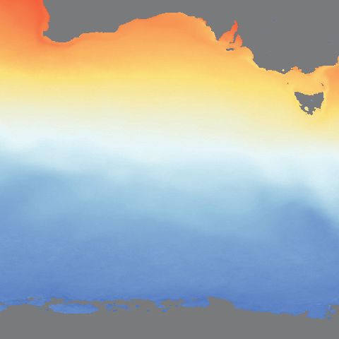
Figure 1. Map of sample sites (dots) relative to major South-
over ∼ 2 h. Thus, these samples represent collections along
ern Ocean fronts (lines) and satellite SST (means for productive
∼ 20 nautical miles of the ship track (except when done at
months, October–March, over the sample collection period 2008–
2014). Front abbreviations: SAF – Subantartic Front; PF: Polar stations).
Front; sACCf: Southern Antarctic Circumpolar Current Front; N: POC/PON samples were filtered through pre-combusted
north; M: middle; S: south. 13 mm diameter quartz filters (0.8 µm pore size, Sartorius
catalogue no. FT-3-1109-013) that had been pre-loaded in
clean (flow-bench) conditions in the laboratory into in-line
polycarbonate filter holders (Sartorius no. 16514E). The fil-
2.1 Voyages and sample collection procedures
ters were preserved by drying in their filter holders at 60 ◦ C
for 48 h at sea and returned to the laboratory in clean dry
The locations of the voyages, divided into north and south boxes.
legs, are shown in Fig. 1. Voyage and sample collection Biogenic silica samples were filtered through either 13 mm
details are given in Table 1, where for ease of reference diameter nitrocellulose filters (0.8 µm pore size, Millipore
we have numbered the legs in chronological order and re- catalogue no. AAWP01300) or 13 mm diameter polycarbon-
fer to them hereafter as VL1, VL2, etc. Samples were col- ate filters (0.8 µm pore size, Whatman catalogue no. 110409),
lected from the Australian icebreaker RV Aurora Australia pre-loaded in clean (flow-bench) conditions in the labora-
for four voyages and from the French Antarctic resupply tory into in-line polycarbonate filter holders (Sartorius no.
vessel l’Astrolabe for one voyage. All samples were col- 16514E). Filters were preserved by drying in their filter hold-
lected from the ships’ underway “clean” seawater supply
lines with intakes at ∼ 4 m depth. These supply lines are
www.biogeosciences.net/15/31/2018/ Biogeosciences, 15, 31–49, 201834 T. W. Trull et al.: Distribution of planktonic biogenic carbonate organisms in the Southern Ocean
ers at 60 ◦ C for 48 h at sea and returned to the laboratory in for POC and PON, respectively. Importantly the processing
clean dry boxes. blanks were large and variable and were corrected for sep-
PIC samples were collected by sequential filtration for arately for each voyage. For VL2 and VL3, POC process
two size fractions. After pre-filtration through a 47 mm di- blanks averaged 25 ± 6 µg C (1 SD, n = 2), equating to 20 %
ameter 1000 µm nylon mesh and supply pressure reduction of the average sample value. For VL4 and VL5, POC process
to 137 kPa, seawater was filtered through a 47 mm diame- blanks averaged 14 ± 2 µg C (1 SD, n = 4), equating to 18 %
ter in-line 50 µm nylon filter to collect foraminifera and then of the average sample value. For VL6 and VL7, POC process
through a 47 mm diameter in-line 0.8 µm GF/F filter (What- blanks averaged 23 ± 3 µg C (1 SD n = 4), equating to 28 %
man catalogue no. 1825-047) to collect coccolithophores. of the average sample value. For VL8 and VL9 POC process
The flow path was split using a pressure relief valve set to blanks averaged 14 ± 1 µg C (1 SD n = 4), equating to 14 %
55 kPa, so that large volumes (∼ 200 L) passed the 50 µm fil- of the average sample value.
ter and only a small fraction of this volume (∼ 15 L) passed
the 0.8 µm filter. Filtration time was typically 2 h. Volume 2.2.2 Biogenic silica analysis
measurement was done by either metering or accumulation.
Based on visual examination, the high flow rate through the Biogenic silica was dissolved by adding 4 mL of 0.2 M
50 µm nylon mesh was sufficient to disaggregate faecal pel- NaOH and incubating at 95 ◦ C for 90 min, similar to the
lets and detrital aggregates. The flow rate data also suggest method of Paasche (1973). Samples were then rapidly cooled
that filter clogging was uncommon (see the Supplement for to 4 ◦ C and acidified with 1 mL of 1 M HCl. Thereafter,
an expanded discussion). While still in their holders, the fil- samples were centrifuged at 1880 g for 10 min and the su-
ters were rinsed twice with 3 mL of 20 mM potassium tetrab- pernatant was transferred to a new tube and diluted with
orate buffer solution (for the first couple of voyages and 36 g L−1 sodium chloride. Biogenic silica concentrations
later degassed deionized water) to remove dissolved inor- were determined by spectrophotometry using an Alpkem
ganic carbon and were blown dry with clean pressurized air model 3590 segmented flow analyser and following USGS
(69 kPa). We consider that the short contact time of this rinse method I-2700-85 with these modifications: ammonium
did not dissolve PIC, based on the sharp (non-eroded) fea- molybdate solution contained 10 g L−1 (NH4 )6 Mo7 O24 ,
tures of coccolithophores collected in this way and examined 800 µL of 10 % sodium dodecyl sulfate detergent replaced
by scanning electron microscopy (Cubillos et al., 2007). The Levor IV solution, acetone was omitted from the ascorbic
filters were then removed from their holders, folded and in- acid solution, and sodium chloride at the concentration of
serted into Exetainer glass tubes (Labco catalogue no. 938W) seawater was used as the carrier solution. Station replicates
and dried at 60 ◦ C for 48 h for return to the laboratory. In had a standard error of 9 % (1 SD n = 9). The average blank
the following text, we refer to the GF/F filter sample re- values were 0.002 ± 0.003 µmoles per filter (1 SD, n = 13)
sults (which sampled the 0.8 (∼ 1) to 50 µm size fraction) as for nitrocellulose filters and 0.002 ± 0.002 µmoles per filter
PIC01 and the nylon mesh sample fraction (which sampled (1 SD, n = 2) for polycarbonate filters, equating to 0.16 and
the 50–1000 µm size fraction) as PIC50. 0.01 % of average sample values, respectively.
2.2 Sample analyses 2.2.3 Particulate inorganic carbon analysis
2.2.1 Particulate organic carbon and nitrogen analysis Particulate inorganic carbon samples were analysed by
coulometry using a UIC CM5015 coulometer connected to
The returned filter holders were opened in a laminar flow a Gilson 232 autosampler and syringe dilutor. The samples
bench. Zooplankton were removed from the filters and the were analysed directly in their gas-tight Exetainer collec-
filters were then cleanly transferred into silver cups (Sercon tion tubes by purging for 5 min with nitrogen gas, acidifi-
catalogue no. SC0037), acidified with 50 µL of 2 NHCl and cation with 1.6 mL (PIC50 – 50 µm nylon filters) or 2.4 mL
incubated at room temperature for 30 min to remove carbon- (PIC01 – GF/F filters) of 1 N phosphoric acid, and equilibra-
ates and dried in an oven at 60 ◦ C for 48 h. The silver cups tion overnight at 40 ◦ C. Samples were analysed the follow-
were then folded closed and the samples, along with pro- ing day with a sample analysis time of 8 min and a dried
cess blanks (filters treated in the same way as samples but carrier gas flow rate of 160 mL min−1 . Calcium carbonate
without any water flow on-board the ship) and casein stan- standards (Sigma catalogue no. 398101-100G) were either
dards (Elemental Microanalysis organic analytical standard weighed onto GF/F filters or weighed into tin cups (Ser-
catalogue no. B2155, batch 114859) were sent to the Uni- con catalogue no. SC1190) and then inserted into Exe-
versity of Tasmania Central Sciences Laboratory for CHN tainer tubes (some with blank nylon filters). Station repli-
elemental analysis against sulfanilamide standards. Repeat cates had standard errors of 18 % (1 SD n = 11) and 13 %
samples collected sequentially at approximately 2 h intervals (1 SD n = 11) for PIC01 and PIC50, respectively. The av-
while the ship remained on station (station replicates) had a erage GF/F filter blank value was −0.07 ± 0.27 µg C (1 SD,
standard error of 7 % (1 SD n = 10) and 8 % (1 SD n = 10) n = 47), equating to −0.21 % of average sample values, and
Biogeosciences, 15, 31–49, 2018 www.biogeosciences.net/15/31/2018/T. W. Trull et al.: Distribution of planktonic biogenic carbonate organisms in the Southern Ocean 35
it was 0.04±0.27 µg C (1 SD, n = 46) for nylon filters, equat- resistant 5 × 8 mm silver cups (Sercon SC0037), treating
ing to 0.05 % of average sample values. these with two 20 µL aliquots of 2 NHCl to remove car-
bonates (King et al., 1998) and drying at 60 ◦ C for at least
2.3 Distinct sample collection and analytical methods 48 h. For the 50 µm mesh filtration samples and the centrifuge
used during V1 samples, 0.5–1.0 mg aliquots of the dried (72 h at 60 ◦ C) cen-
trifuge pellet remaining after PIC coulometry were encapsu-
2.3.1 Distinct sample collection procedures for VL1 lated in 4 × 6 mm silver cups (Sercon SC0036). Analyses of
all these sample types was by catalytic combustion using a
For VL1, single samples were collected at each location by Thermo-Finnigan Flash 1112 elemental analyser calibrated
both sequential filtration and centrifugation of the underway against sulfanilamide standards (Central Sciences Labora-
supply over 1–3 h. Despite the long collection times, these tory, University of Tasmania). The precision of the analysis
samples are effectively point samples because they were col- was ±1 %. A blank correction of 0.19 ± 0.09 µg C was ap-
lected on station. plied, which represented 1.6 % of an average sample.
Sequential filtration was done using in-line 47 mm filter PIC concentrations were determined for subsamples of
holders (Sartorius Inc.) holding three sizes of nylon mesh the 0.8 µm GF/F filters (half of the filter), the whole 50 µm
(1000, 200, 50 µm) followed by a glass fibre filter (Whatman mesh screens and the whole centrifuge samples by closed
GF/F, 0.8 µm nominal pore size; muffled before use). These system acidification and coulometry using a UIC CM5011
size fractions were intended to collect foraminifera (50– CO2 coulometer. The samples were placed in glass vials (or
200 µm) and coccolithophores (0.8–50 µm) and pteropods in the case of the centrifuge tubes connected via an adap-
(200–1000 µm), but the largest size fraction had insufficient tor), connected to a manual acidification unit and condenser
material for analysis. The flow rate at the start of filtra- and maintained at 40 ◦ C after acidification with 4 mL of 1
tion was 25–30 L h−1 and typically dropped during filtra- NHCl and swept with a nitrogen gas flow (∼ 100 mL min−1 )
tion. The 0.8 µm filter was replaced if flow rates dropped be- via a drier and aerosol filter (Balston) into the coulometry
low 10 L h−1 . Sampling typically took 3 h. Quantities of fil- cell. Calibration versus calcium carbonate standards (200 to
tered seawater were measured using a flowmeter (Magnaught 3000 µg) provided a precision of ±0.3 %. However, for the
M1RSP-2RL) with a precision of ±1 %. After filtration, any 0.8 µm filter, precision was limited to 10 % by subsampling
remaining seawater in the system was removed using a vac- of the filter due to uneven distribution. Blank corrections
uum pump. Filters were transferred to 75 mm Petri dishes were applied to the 0.8 µm size fraction, being 2.4 ± 1.8 µg C
inside a flow bench, placed in an oven (SEM Pty Ltd, vented and representing 8.8 % of an average sample. The 50 µm frac-
convection) for 3–6 h to dry at 60 ◦ C and stored in dark, cool tion blank correction was 3.3±0.1 µg C, representing 22 % of
boxes for return to the laboratory. an average sample. Centrifuge pellet coulometry blank sub-
A continuous-flow Foerst-type centrifuge (Kimball Jr. and traction was 2.0 ± 0.1 µg C, equivalent to 2.8 % of an average
Ferguson Wood, 1964), operating at 18 700 rpm, was used sample.
to concentrate phytoplankton from the underway system at Biogenic silica analysis of the residues remaining after
a flow rate of 60 L per hour, measured using a water meter PIC analysis of the centrifugation samples was by alkaline
with a precision of ±1 % (Arad). Sampling typically took digestion (0.2 N NaOH) in a 95 ◦ C water bath for 90 min,
1–3 h. After centrifugation, 500 mL of deionized water was similar to the method described by Paasche (1973) and as
run through the centrifuge to flush away any remaining sea- described in Sect. 2.2.2. with the variation that 4 mL of each
water and associated dissolved inorganic carbon. This was sample was transferred from the centrifuge tubes and filtered
followed by 50 mL of ethanol to flush away the deionized using a syringe filter before dilution to 10 mL.
water, ensure organic matter detached from the cup wall and
speed subsequent drying. Inside a laminar flow clean bench, 2.3.3 Comparison of VL1 to other voyages
the slurry in the centrifuge head was transferred into a 10 mL
polypropylene centrifuge tube (Labserve) and the material The first survey on VL1 in 2008 differed from later efforts
on the wall of the cup was transferred using 3 mL of ethanol in two important ways: (i) POC and PIC samples were col-
and a rubber policeman. The sample was then centrifuged for lected by both filtration and centrifugation, (ii) separate BSi
15 min and 3200 rpm, and the supernatant (∼ 7 mL) was re- samples were not collected – instead BSi analyses were car-
moved and discarded. The vial was placed in the oven to dry ried out only on the sample residues from PIC coulometric
for 12 h at 60 ◦ C and returned to the laboratory. sample digestions of the centrifuge samples. Comparison of
POC and PIC results from the centrifugation samples (effec-
2.3.2 Distinct analytical procedures for VL1 samples tively total samples without size fractionation) and the filtra-
tion samples (separated into the PIC01 0.8–50 µm and PIC50
POC/PON analyses for the 0.8 µm size fraction collected by 50–1000 µm size fractions) shows (Fig. 2) that filtration col-
filtration were done by packing five 5 mm diameter aliquots lected somewhat more PIC (on the order of 20–30 %) and
(punches) of the 47 mm diameter GF/F filters into acid- considerably more POC (on the order of 200–300 %) than
www.biogeosciences.net/15/31/2018/ Biogeosciences, 15, 31–49, 201836 T. W. Trull et al.: Distribution of planktonic biogenic carbonate organisms in the Southern Ocean
16 2.4 Analysis of nutrients, dissolved inorganic carbon,
(a)
POC alkalinity, and calculation of pH and calcite
14
1 : 1 line saturation
12
Filtration (µM)
10
Nutrients were analysed on-board ship for VL1 to VL5
and on frozen samples returned to land for VL6–9,
8 all by the Commonwealth Scientific and Industrial Re-
6 search Organisation (CSIRO) hydrochemistry group follow-
ing WOCE/CLIVAR standard procedures, with minor varia-
4
tions (Eriksen, 1997), to achieve precisions of ∼ 1 % for ni-
2 trate, phosphate and silicate concentrations. Dissolved inor-
0
ganic carbon (DIC) and alkalinity samples were collected in
0 1 2 3 4 5 6 7 8 gas-tight bottles poisoned with mercuric chloride and mea-
Centrifugation (uM) sured at CSIRO by coulometry and open-cell titration, re-
spectively (Dickson et al., 2007). Comparison to certified ref-
erence materials suggests an accuracy and precision for both
DIC and alkalinity of better than ±2 µmol kg−1 . Full details
0.45 have recently been published (Roden et al., 2016). Calcula-
(b) tions of pH (free scale) and calcite saturation were based on
0.40
the Seacarb version 3.1.2 software (https://CRAN.R-project.
0.35 PIC (GF/F+50 µm mesh)
org/package=seacarb), which uses the default selection of
PIC (GF/F)
0.30 equilibrium constants given in Van Heuven et al. (2011).
1 : 1 line
Filtration (µM)
0.25
0.20
2.5 Satellite-derived ocean properties and the NASA
Ocean Biogeochemistry Model
0.15
0.10 The locations of oceanographic fronts in the Australian sec-
0.05 tor were estimated from satellite altimetry, following the
0.00
approach of Sokolov and Rintoul (2002), updated as fol-
0.00 0.05 0.10 0.15 0.20 lows. Absolute sea surface height (SSH) was calculated by
Centrifugation (µM) adding the sea surface height anomaly from Archiving, Val-
idation and Interpretation of Satellite Oceanographic data
Figure 2. Comparison of centrifugation versus filtration size-
(AVISO+) (Pujol et al., 2016) to the 2500 dbar reference
fraction results for voyage leg 1: (a) centrifugation total POC ver-
sus filtration POC (0.8–50 µm fraction); (b) centrifugation total PIC level mean dynamic topography of Olbers et al. (1992). The
versus filtration PIC01 (0.8–50 µm) and PIC50 (50–1000 µm) frac- positions of the fronts were then identified using the sea sur-
tions. face height contours corresponding to the positions of the
Southern Ocean fronts identified by Sokolov and Rintoul
(2007a) in the region 100–180◦ E. From this analysis, we
show eight fronts from north to south consisting of the fol-
centrifugation. This fits with the possibility of the loss of lowing.
material from the continuous centrifuge cup, with a greater – Fronts 1–3: north, middle and south branches of the
loss of lower-density organic matter (and a possible addi- Subantarctic Front (SAF), which bound the highest-
tional loss of organic matter via dissolution in the ethanol velocity jets of the Antarctic Circumpolar Current
rinsing step). Thus, for a comparison of VL1 POC and PIC to (ACC).
the other voyages, we use only the filtration results, thereby
avoiding methodological biases. For BSi, we do not have this – Fronts 4–6: north, middle and south branches of the Po-
possibility. Based on the low centrifuge yields for PIC and lar Front (PF), associated with subsurface temperature
POC, we can expect that the VL1 BSi values are also too features related to the strength of the ACC and with
low. This is confirmed by comparison to the other voyages, the shoaling of Circumpolar Deep Water (CDW) in the
which reveals that VL1 BSi values were lower than those of overturning circulation. The Polar Frontal Zone (PFZ)
other voyages, especially in the far south where BSi values lies between the northernmost of these branches and the
were generally highest (data shown below) but nonetheless SAF to its north.
had similar north–south latitudinal trends. For this reason,
our further interpretation of the VL1 BSi results is only in – Fronts 7–8: north and south branches of the South-
terms of these latitudinal trends. ern Antarctic Circumpolar Current Front (sACCf) front,
Biogeosciences, 15, 31–49, 2018 www.biogeosciences.net/15/31/2018/T. W. Trull et al.: Distribution of planktonic biogenic carbonate organisms in the Southern Ocean 37
marking weaker flows in Antarctic waters of the ACC it only for context and not for any detailed comparisons to
and occurring near where upwelling of old nutrient-rich shipboard observations. We refer to these estimates as satel-
and relatively acidic Circumpolar Deep Water comes lite chlorophyll (SChl) values.
closest to the surface. Particulate inorganic carbonate concentrations
(mol m−3 ) based on backscatter magnitudes (Balch
We do not show the Subtropical Front (STF), which marks et al., 2005) were obtained from the NASA
the northern boundary of the Southern Ocean, or the South- MODIS Aqua ocean colour product available online:
ern Boundary Front, which marks the southern edge of the https://oceancolor.gsfc.nasa.gov/cgi/l3/A20111212011151.
ACC (separating it from westerly flow in Antarctic shelf wa- L3m_MO_PIC_pic_9km.nc.png?sub=img (NASA Goddard
ters). This is because both features have weak, discontinuous Space Flight Center, 2014b).
SSH signatures south of Australia: mesoscale eddies rather We refer to these estimates as SPIC values. The veracity of
than the STF dominate the weak SSH field in the Subantarc- these estimates in the Southern Ocean remains an active area
tic Zone (SAZ; between the STF and the SAF), and the detec- of research. PIC sampling in the subantarctic South Atlantic
tion of the Southern Boundary Front is confounded by prox- found levels 2–3 times lower than the satellite estimates
imity to the Antarctic shelf, where altimetry is impacted by (Balch et al., 2011), and the algorithm also produces sur-
other processes, including sea-ice cover for much of the year prisingly high estimates in Antarctic waters, where limited
(Sokolov and Rintoul, 2007a). shipboard surveys suggest that coccolithophore abundances
We considered using these dynamic heights and front lo- drop strongly (work summarized in Balch et al., 2005). Our
cations as ordinates for the spatial distributions of POC, PIC data provide the most extensive PIC observations for com-
and BSi. In the core of the ACC (50–60◦ S), this did help parison to SPIC values in Antarctic waters yet available, and
explain some departures from monotonic north–south trends this is discussed in detail below. The comparison of PIC and
as resulting from meanders of the fronts, but latitude was SPIC values at individual sampling sites was based on com-
more strongly correlated with PIC abundance in the SAZ and bined data from MODIS Aqua and Terra 9 km daily products.
with BSi in southern ACC waters and Antarctic shelf waters, SPIC values were an average of pixels within 25 km of PIC
where dynamic height contours were only weakly varying. sampling sites on the same day.
Accordingly, there was no overall advantage of replacing lat- The phytoplankton function type model is based on Gregg
itude by dynamic height as a predictor of biogenic mineral and Casey (2007a). Details of particular relevance to com-
concentrations, and we have used latitude as the ordinate in parisons with our observations are discussed in Sect. 3.4.
our figures and discussion.
Sea surface temperatures (◦ C) – e.g. see Fig. 1 – were ob-
tained from the NASA MODIS Aqua 11 µm night-only L3m 3 Results and discussion
product available online:
https://giovanni.gsfc.nasa.gov/giovanni/#service= 3.1 Representativeness of oceanographic sampling
TmAvMp&starttime=&endtime=&data=MODISA_L3m_
SST_2014_nsst&variableFacets=dataFieldMeasurement% As shown in Fig. 1, sampling covered all Southern Ocean
3ASea%20Surface%20Temperature%3B zones from subtropical waters in the north to seasonally
We chose the night values to avoid shallow ephemeral sea-ice-covered waters in the south (covering SST ranging
structures arising from daytime solar heating. We refer to from −1 to 23 ◦ C). Almost all samples were representa-
these estimates simply as sea surface temperature (SST) val- tive of high-nutrient low-chlorophyll Southern Ocean wa-
ues. ters, indicative of iron limitation. Exceptions occurred near
Phytoplankton chlorophyll concentrations (Chl in Tasmania, where moderate levels of SChl were occasionally
mg m−3 =µg L−1 ) were obtained from the NASA MODIS present, and over the Antarctic shelf where locally very high
Aqua L3m product available online: https://giovanni. levels of SChl were present. Individual maps for each voy-
gsfc.nasa.gov/giovanni/#service=TmAvMp&starttime= age leg of SChl are provided in the Supplement and those of
&endtime=&data=MODISA_L3m_CHL_2014_ satellite reflectance-based estimates of PIC (SPIC) are found
chlor_a&variableFacets=dataFieldMeasurement% below, and they reveal that higher values of SChl and SPIC
3AChlorophyll%3B (NASA Goddard Space Flight Center, are often associated with mesoscale structures, especially in
2014a). the Subantarctic and Polar Frontal zones. This means that
The algorithm relies on the blue/green reflectance ratio for mesoscale variability makes satellite-versus-shipboard com-
Chl values above 0.2 µg L−1 and incorporates stray light cor- parisons difficult, and this problem is exacerbated by fre-
rection based on the difference between red and blue light quent cloud cover. Both techniques characterize the very
reflectances at lower Chl levels. This product has been sug- upper water column, with ship samples from ∼ 4 m depth
gested to underestimate chlorophyll in the Southern Ocean and the satellite ocean colour observations reflecting the e-
south of Australia (Johnson et al., 2013) but has the advan- folding penetration depth of ∼ 10–15 m (Grenier et al., 2015;
tage of ongoing ready availability. For this reason, we use Morel and Maritorena, 2001).
www.biogeosciences.net/15/31/2018/ Biogeosciences, 15, 31–49, 201838 T. W. Trull et al.: Distribution of planktonic biogenic carbonate organisms in the Southern Ocean
VL1 VL2 VL3
10
0.1
0.001
VL4 VL5 VL6
10
Concentration μmoles kg−1
0.1
0.001
VL7 VL8 VL9
10
0.1
POC
BSi
0.001 PIC01
PIC50
−60 −50 −40 −60 −50 −40 −60 −50 −40
Latitude
Figure 3. Latitudinal variations in POC, BSi, PIC50 and PIC01 concentrations for each voyage leg. See Table 1 for voyage leg details and
Fig. 1 for sample sites.
It appears likely that our single-depth sampling can be 3.2 Latitudinal distributions of BSi, PIC and POC
considered as representative of upper water column phyto-
plankton concentrations because pigment samples and pro- All the voyage legs exhibited similar latitudinal variations in
files of beam attenuation and nighttime fluorescence from the measured chemical components (Fig. 3). BSi, predomi-
some of these voyages as well as previous work show that nantly derived from diatoms, was clearly the dominant bio-
biomass is generally well mixed in the upper water column genic mineral in the south in Antarctic waters. PIC01 concen-
and that when subsurface chlorophyll maxima are present trations, predominantly derived from coccolithophores, were
they primarily reflect increased chlorophyll levels rather than highest in northern subantarctic waters, although even there
increased phytoplankton abundances (Bowie et al., 2011a, b; BSi was often present at similar levels. Interestingly, PIC50
Parslow et al., 2001; Rintoul and Trull, 2001; Shadwick et concentrations, predominantly derived from foraminifera, of-
al., 2015; Trull et al., 2001b; Wright et al., 1996; Wright ten exhibited maxima in the middle of the Southern Ocean at
and van den Enden, 2000). This perspective is also consis- latitudes of 55–60◦ S. The latitudinal variations in all these
tent with the limited information on the depth distributions biogenic mineral concentrations were quite strong, exceed-
of coccolithophores in the Southern Ocean, which generally ing 2 orders of magnitude. In contrast, variations in POC
exhibit relatively uniform and maximal values (especially for were 10-fold smaller and often quite uniform across the
the most abundant species, Emiliania huxleyi) within the sur- central Southern Ocean, with maxima sometimes in the far
face mixed layer (Findlay and Giraudeau, 2000; Holligan et north near Tasmania and sometimes in the far south over
al., 2010; Mohan et al., 2008; Takahashi and Okada, 2000). the Antarctic shelf (Fig. 3). Variations in BSi, PIC and POC
There is some evidence that this conclusion can also be ap- concentrations among the voyages, at a given latitude, were
plied to the PIC50 foraminiferal fraction, in that the most smaller than these north–south trends. It seems likely that
abundant of these organisms tend to co-locate with phyto- these smaller variations were partly seasonal, in that the ear-
plankton in the mixed layer in the Southern Ocean (Mortyn liest seasonal voyage leg (VL4 in September) had lower
and Charles, 2003). concentrations of every component. But across the other
voyages, ranging from mid-November (VL5) to mid-April
(VL1), no clear seasonal cycle was exhibited, perhaps owing
to variations in sampling location, and the known importance
of interannual and mesoscale structures in Southern Ocean
Biogeosciences, 15, 31–49, 2018 www.biogeosciences.net/15/31/2018/T. W. Trull et al.: Distribution of planktonic biogenic carbonate organisms in the Southern Ocean 39
(a) renewal of silica supply from upwelled deep waters in the
10 000
Southern Ocean that are carried north by Ekman transport,
combined with the recycling of biogenic silica within sur-
face waters, given that by midsummer silicate is largely de-
pleted north of the Subantarctic Front (Nelson et al., 2001;
100
Trull et al., 2001b). Accordingly the relative dominance of
–1
diatoms and coccolithophores in the SAZ may be quite sen-
mol mol
sitive to changes in the overturning circulation and westerly
1 wind field. How this might translate into impacts on the bi-
ological carbon pump remains far from clear. Interestingly,
deep ocean sediment traps in the SAZ south of Australia re-
0.01 veal a strong dominance (4-fold) of PIC over BSi in the ex-
POC/(PIC01+PIC50) port flux to the ocean interior, reminding us that export can
BSi/PIC01
be selective (and also that foraminifera can contribute a sig-
(b)
nificant fraction of total PIC, estimated to vary from ∼ 1/3
100 to 2/3; King and Howard, 2003). The POC flux recovered
by these deep sediment traps was close to the global median
and similar to that of biogenic silica-dominated fluxes in the
10 Polar Frontal Zone to the south (Trull et al., 2001a).
The importance of diatoms across the entire Southern
% of total POC
Ocean, relative to coccolithophores, is further emphasized
1
by expressing their biogenic mineral abundances in terms
of associated POC, using average values for the POC/BSi
ratio of iron-limited diatoms (3.35, equivalent to a Si / N
0.1
ratio of 2 and a Redfield C / N ratio of 6.7; Ragueneau et
al., 2006; Takeda, 1998) and the POC / PIC ratio of coc-
Diatom POC
Cocco POC colithophores (1.5, for Emiliania huxleyi morphotype A, the
−60 −50
Latitude
−40 dominant Southern Ocean species; Bach et al., 2015; Muller
et al., 2015). As shown in Fig. 4b, this suggests that diatoms
Figure 4. Latitudinal variations in the dominance of diatoms dominate the accumulation of organic carbon throughout the
versus coccolithophores and their contributions to total POC Southern Ocean, with coccolithophores generally contribut-
for results combined from all voyages: (a) BSi / PIC01 and ing less than half that of diatoms in the SAZ and less than a
POC / (PIC50 + PIC01) ratios; (b) percent contributions to total tenth of that in Antarctic waters. This statement is of course
POC attributable to diatoms (assuming POC / BSi = 3.35) and coc- limited to POC captured by our small-volume, size-limited
colithophores (assuming POC / PIC01 = 0.833).
(1–1000 mm) sampling procedure, and variability in the ex-
tent of dominance and the scaling of POC to biogenic min-
erals still allows significant contributions from other POC
phytoplankton distributions (e.g. Moore et al., 1999; Moore sources. The relatively small POC contribution from coc-
and Abbott, 2002; Sokolov and Rintoul, 2007b). As noted colithophores is only weakly sensitive to the ∼ 3-fold vari-
in the Sect. 2.3, the BSi values for VL1 stand out as being ation (Muller et al., 2015) of POC / PIC ratios among Emil-
too low, in that they were well below those of other voyages, iania huxleyi morphotypes. Using the lower value of 0.83
while the POC, PIC01 and PIC50 values were similar. observed for over-calcified forms that occur in the north-
The latitudinal dependence of the relative importance of ern SAZ would reduce the POC contribution there but still
diatoms and coccolithophores is revealed by viewing the leave it co-dominant with diatoms, and using the higher value
BSi/PIC01 ratios as an ensemble for all the voyages (the use of 2.5 observed for polar morphotype C would increase the
of the ratio helps to remove seasonal and interannual vari- POC contribution in Antarctic waters but still leave it over-
ations in their abundances, which tend to track each other whelmed by the diatom contribution (Fig. 4b). The relative
at a given latitude). The BSi/PIC01 ratio reaches values of contributions to total POC are also sensitive to the POC / BSi
200 in the far south and decreases north of 50◦ S to val- ratio chosen for diatoms (which vary significantly across
ues near 1 (Fig. 4a). The approximate equivalence of BSi genera; Ragueneau et al., 2002, 2006). For these reasons, the
and PIC01 occurs relatively far north in the Southern Ocean, relative dominance is best viewed on the log scale of Fig. 4b
near 50◦ S, and thus near the southern edge of the Subantarc- and while keeping in mind the considerable scatter.
tic Zone. This persistence of the importance of diatoms as a Figure 4b also emphasizes that total POC contents can
major component of the phytoplankton community in north- be largely explained by diatom biomass in Antarctic waters
ern waters of the Southern Ocean must reflect the wintertime (south of 50◦ S), whereas in the SAZ (north of 50◦ S), total
www.biogeosciences.net/15/31/2018/ Biogeosciences, 15, 31–49, 201840 T. W. Trull et al.: Distribution of planktonic biogenic carbonate organisms in the Southern Ocean
POC often exceeds the sum of contributions from diatoms of mesoscale circulation, ephemeral inputs of the limiting nu-
and coccolithophores. This serves as an important reminder trient iron and food web dynamics produce variability that
that other organisms are important to the carbon cycle in cannot be adequately assessed in this way, leaving sparse
the SAZ, and phytoplankton functional type models should sampling open to potentially large biases. The use of satellite
avoid overemphasis on diatoms and coccolithophores just be- observations is clearly the path forward to alleviate this prob-
cause they have discernable biogeochemical impacts (on sil- lem, and the development of algorithms for global coccol-
ica and alkalinity, respectively) and satellite remote-sensing ithophore distributions has been a major advance (Balch et
signatures (Hood et al., 2006; Moore et al., 2002). Finally, we al., 2005; Brown and Yoder, 1994). Until recently the calibra-
note that the relatively low levels of PIC across the Southern tion of these SPIC values has been based primarily on North
Ocean as observed here means that POC / PIC ratios are high Atlantic observations. Work to check these efforts for the
– greater than 4 in the SAZ and ranging up to 20 in Antarctic Southern Ocean has begun but remains sparse. Early work in
waters (Fig. 4a). This suggests that calcification has a neg- the South Atlantic found that SPIC values appeared to exceed
ligible countering impact on the reduction of surface ocean ocean PIC by a factor of 2–3 (Balch et al., 2011), and based
CO2 partial pressure by phytoplankton uptake, even smaller on a handful of samples, it was suggested that this might re-
than the influence of a few percent to ∼ 10 % identified ear- flect a lower amount of PIC per coccolith (Holligan et al.,
lier from deep sediment trap compositions in high-nutrient, 2010), and it has since been confirmed that polar coccol-
low-chlorophyll (HNLC) (Boyd and Trull, 2007a) and iron- ithophores can have low PIC contents (Charalampopoulou
enriched waters, respectively (Salter et al., 2014). et al., 2016; Muller et al., 2015; Poulton et al., 2011). Two
Notably, our Southern Ocean PIC01 estimates are smaller dedicated voyages to investigate the Great Calcite Belt in
than those found in Northern Hemisphere polar waters. As the SAZ and PFZ across the South Atlantic and south Indian
compiled by Balch et al. (2005), concentrations were 100- oceans attempted a comparison of acid-labile backscatter (as
fold higher (∼ 10 µM) in the north Atlantic south of Iceland a proxy for PIC) and MODIS SPIC values, but there were no
(60–63◦ N) than any of our values and 1000-fold higher than matchups in the South Atlantic owing to cloudy conditions
our values in the same Southern Hemisphere latitude range. (Balch et al., 2016). Results from the South Indian sector
Values collected over many years from the Gulf of Maine and from other voyages in the South Atlantic show high acid-
(Balch et al., 2008) were ∼ 1 µM and thus 5–10 times higher labile backscatter, which translates into high SPIC estimates
than our SAZ values (Gulf of Maine summer temperatures in the SAZ and PFZ (especially in naturally iron-fertilized
are similar to the SAZ, and temperatures are colder in win- waters) but also high values further south which are not in
ter). This difference between hemispheres is also evident in agreement with ship observations (Balch et al., 2016; Smith
observations from the South Atlantic, where PIC values esti- et al., 2017).
mated from acid labile backscatter for six voyages between The comparison of our ship observations to MODIS SPIC
2004 and 2008 and latitudes 40–50◦ S were ∼ 0.1–0.5 µM estimates are shown in Fig. 5 for each voyage leg. These
in remote waters (Balch and Utgoff, 2009), increasing to reveal some agreement in the SAZ in terms of identifying
1–2 µM in the Argentine Basin with a few values reaching moderate levels of PIC, often in association with higher lev-
4 µM (Balch et al., 2014). These high South Atlantic ob- els of total SChl (Supplement) but differ strongly in Antarc-
servations are the highest of the Great Calcite Belt, identi- tic waters where all ship observations reveal low PIC values,
fied as a circumpolar feature of subantarctic waters based whereas the SPIC estimates in Antarctic waters reach and
on SPIC values (Balch et al., 2014, 2011). Notably, ship- often exceed those in the SAZ, especially over the Antarc-
board PIC measurements in this feature are 2–3 times lower tic shelf. Both cloudy conditions and strong mesoscale vari-
than the SPIC estimates in the South Atlantic (Balch et al., ability limit the number of direct comparisons (matchups)
2011), and ship-collected samples from two voyages across that can be made. Using a matchup length scale of 25 km
the South Atlantic and Indian sectors (Balch et al., 2016) (i.e. the ship and satellite observations must be within 25 km
exhibit PIC concentrations (actual PIC values accessed on- of each other on the same day), which is somewhat larger
line at http://www.bco-dmo.org/dataset/560357, rather than than the correlation length scale for chlorophyll in the South-
the PIC estimates from acid-labile backscatter shown in the ern Ocean of 10–15 km (Haëntjens et al., 2017), allowed us
paper) that decrease eastwards in this feature to reach values to retain 116 matchups. These results, shown in Fig. 6, con-
close to our observations in the Australian sector of ∼ 0.1 µM firm that the satellite SPIC values are reasonable estimates
(Fig. 3). in subantarctic waters, within a factor of 2–3 (Balch et al.,
2011), but very much too high in Antarctic waters.
3.3 Comparison to satellite PIC (SPIC) estimates
3.4 Comparison to possible environmental controls on
As is very evident from the limited observations we have coccolithophore growth rates
achieved from our efforts over many years, it will never be
possible to characterize Southern Ocean phytoplankton pop- The ship observations provided here offer a significant ad-
ulation dynamics from ship-based sampling – the influences vance in quantifying the distributions of coccolithophores in
Biogeosciences, 15, 31–49, 2018 www.biogeosciences.net/15/31/2018/T. W. Trull et al.: Distribution of planktonic biogenic carbonate organisms in the Southern Ocean 41 Figure 5. Maps comparing ship-based distributions of coccolithophore PIC distributions (PIC01; coloured dots) with satellite PIC esti- mates (SPIC; background colours) for each voyage leg. The SPIC estimates are averages for the month preceding the start of each voyage leg. Contour lines indicate dynamic height-determined frontal positions for the week preceding the each voyage leg (see Fig. 1 for front nomenclature). the Southern Ocean south of Australia but much less under- mer I9 northward hydrographic section from Antarctica to standing of why these distributions arise and therefore how Perth) and VL6 (the early summer to midsummer southward they might change in response to climate, circulation and bio- l’Astrolabe transit from Tasmania to Antarctica). VL3 cov- geochemical changes in the future. Coccolithophores, espe- ered the widest range of physical properties and exhibited cially the most common species Emiliania huxleyi, have been PIC01 concentrations that remained elevated further south studied sufficiently in the laboratory to allow possible im- than any other voyage (Fig. 3). VL6 exhibited the more typ- portant controls on their niches and especially their calcifica- ical PIC01 distribution of a close to continuous decrease tion rates to be proposed, including temperature, pH, pCO2 , southward (Fig. 3). The results from the other voyage legs calcite saturation state, light, and macro- and micronutrient were very similar to VL3 (figures not shown; data available availability (Bach et al., 2015; Feng et al., 2016; Mackinder in the Supplement). et al., 2010; Muller et al., 2015; Müller et al., 2017; Schlüter Many properties that might influence coccolithophore pro- et al., 2014; Schulz et al., 2007; Sett et al., 2014; Zhang et al., ductivity decreased strongly and close to monotonically from 2015). We collected observations of many of these properties north to south across the Southern Ocean for our voyages in parallel with our PIC observations and now briefly exam- (Fig. 7). These include temperature (from 23 to −0.4 ◦ C for ine whether they present correlations that might contribute our samples), salinity (from 35.6 to 33.6, with a close cor- to understanding why coccolithophores are found mainly in relation with alkalinity; not shown – data available in the northern subantarctic waters and not further south. For illus- Supplement), pH (from 8.20 to 8.08 on the free scale) and trative purposes, we focus on VL3 (the mid- to late sum- the saturation state of calcite (from 5.22 to 2.12). The strong www.biogeosciences.net/15/31/2018/ Biogeosciences, 15, 31–49, 2018
42                       T. W. Trull et al.: Distribution of planktonic biogenic carbonate organisms in the Southern Ocean

                                                                             a strain isolated from subantarctic waters south of Tas-
                                                                             mania (Müller et al., 2017) to provide what might be
                                                                             considered the best current model for the calcification
                                                                             rate response to changing inorganic carbon abundance
                                                                             and speciation, following Eq. (1):

                                                                             Bach relative calcification rate
                                                                                  = a[HCO−            −
                                                                                         3 ]/(b + [HCO3 ]) − e
                                                                                                               −c[CO2 ]
                                                                                                                        − d[H+ ].
                                                                                                                               (1)

                                                                         2. The “Langdon model” based on a simple, inorganic
                                                                            precipitation-motivated parameterization of calcifica-
                                                                            tion as a function of calcite saturation state  (Gat-
                                                                            tuso et al., 1998; Langdon et al., 2000), which has been
                                                                            shown to apply in an approximate way to many corals
                                                                            (Anthony et al., 2011; Silverman et al., 2007) and per-
                                                                            haps to Southern Ocean foraminifera (Moy et al., 2009).
                                                                            We have chosen the simple linear form (n = 1) and a
                                                                            sensitivity at the top end of the observed range (a = 1/4,
                                                                            so that the calcification rate varies linearly from 0 to 1
Figure 6. Comparison of satellite SPIC and ocean PIC concentra-             for  = 1 to 4), following Eq. (2):
tions for the 116 matchups for which satellite SPIC estimates were
available within 25 km of the ocean PIC sample sites, on the same
day. Colours indicate sample latitudes and show that good correla-
tion occurs in subantarctic waters, but there is a strong overestima-        Langdon relative calcification rate = a( − 1)n .    (2)
tion by the satellite technique in Antarctic waters.
                                                                        As shown in Fig. 7, both these calcification rate models ex-
                                                                        hibit limited variations with latitude in the Southern Ocean.
correlation of these properties means that it is not easy to            The Bach model suggests a negligible change in the calcifi-
separate their possible influences on coccolithophore distri-           cation rate. This is essentially because the Southern Ocean
butions without relying on specific thresholds or quantitative          variations in bicarbonate, CO2 and pH are very small com-
response models. This problem of correlations among drivers             pared to the future expected values used in incubation ex-
has been noted before in examining transect data across the             periments. In addition, southward cooling causes pH to rise,
Drake Passage, where more detailed measurements of coc-                 offsetting the impact of a southward decrease in salinity and
colithophore properties augmented with incubation studies               alkalinity, thus reducing the southward decrease in pH and
found that temperature and light were the most probable                 the associated drop in the modelled calcification rate. The
drivers of coccolithophore abundance and calcification rates            Langdon model suggests an approximately 3-fold decrease
(Charalampopoulou et al., 2016). Our lack of information on             in the calcification rate, which is considerably smaller than
the availability of light (mixed layer depth was determined             the more than 10-fold drop in PIC01 (shown on a linear scale
only on the two hydrographic sections), iron, or individ-               in Fig. 7 and a logarithmic scale in Fig. 3). The shape of
ual species and strains makes deducing a possible influence             the Langdon model decrease shows some agreement with
of ocean acidification on coccolithophore distributions from            that of PIC01 for VL6 but none for VL3 (which exhibits
our spatial distribution data even more difficult. Nonetheless,         relatively constant significant PIC01 concentrations in the
we offer a few pertinent observations. Firstly, the change in           40–50◦ S latitude range where the Langdon model shows a
PIC01 abundances with latitude is much larger than expected             strong decrease in the calcification rate, and then a strong
from models of the responses of calcification rates (normal-            drop in PIC01 south of 60◦ S, where the Langdon model
ized to maximum rates) to inorganic carbon system varia-                shows no change). Thus, and unsurprisingly, coccolithophore
tions (Fig. 7). Two models are shown:                                   abundances are clearly not controlled by inorganic carbon
                                                                        chemistry alone. This perspective has been strongly empha-
  1. The “Bach model” based on independent terms for sen-               sized previously, including by Bach et al. (2015), who noted
     sitivity to bicarbonate, CO2 and pH. It fits quite well the        “great care must be taken when correlating carbonate chem-
     results from many laboratory incubations of Emiliania              istry with coccolithophore dispersal because this is by no
     huxleyi strains under conditions of modern and elevated            means the only parameter controlling it. Physical (e.g. tem-
     pCO2 (Bach et al., 2015), and we have used values for              perature), other chemical (e.g. nutrient concentrations), or
     the constants (a, b, c, d) obtained from incubations of            ecological (e.g. grazing pressure) factors will under many if

Biogeosciences, 15, 31–49, 2018                                                                www.biogeosciences.net/15/31/2018/
You can also read