DUKweb: Diachronic word representations from the UK Web Archive corpus
←
→
Page content transcription
If your browser does not render page correctly, please read the page content below
DUKweb: Diachronic word representations from
                                               the UK Web Archive corpus
arXiv:2107.01076v1 [cs.CL] 2 Jul 2021

                                                       Adam Tsakalidis1,2 , Pierpaolo Basile3
                                         Marya Bazzi1,4,5 , Mihai Cucuringu1,5 , and Barbara McGillivray*1,6
                                                                          July 5, 2021

                                            1. The Alan Turing Institute, London, United Kingdom 2. Queen Mary
                                        University of London, London, UK 3. University of Bari, Bari, Italy 4. Univer-
                                        sity of Warwick, Coventry, United Kingdom 5. University of Oxford, Oxford,
                                        United Kingdom 6. University of Cambridge, Cambridge, United Kingdom
                                        *corresponding author: bm517@cam.ac.uk
                                                                            Abstract
                                                 Lexical semantic change (detecting shifts in the meaning and usage of
                                             words) is an important task for social and cultural studies as well as for
                                             Natural Language Processing applications. Diachronic word embeddings
                                             (time-sensitive vector representations of words that preserve their mean-
                                             ing) have become the standard resource for this task. However, given the
                                             significant computational resources needed for their generation, very few
                                             resources exist that make diachronic word embeddings available to the
                                             scientific community.
                                                 In this paper we present DUKweb, a set of large-scale resources de-
                                             signed for the diachronic analysis of contemporary English. DUKweb
                                             was created from the JISC UK Web Domain Dataset (1996-2013), a very
                                             large archive which collects resources from the Internet Archive that were
                                             hosted on domains ending in ‘.uk’. DUKweb consists of a series word co-
                                             occurrence matrices and two types of word embeddings for each year in
                                             the JISC UK Web Domain dataset. We show the reuse potential of DUK-
                                             web and its quality standards via a case study on word meaning change
                                             detection.

                                        1    Background & Summary
                                        Word embeddings, dense low-dimensional representations of words as real-number
                                        vectors [23], are widely used in many Natural Language Processing (NLP) ap-
                                        plications, such as part-of-speech tagging, information retrieval, question an-
                                        swering, sentiment analysis, and are employed in other research areas, including
                                        biomedical sciences [28] and scientometrics [1]. One of the reasons for this
                                        success is that such representations allow us to perform vector calculations in
geometric spaces which can be interpreted in semantic terms (i.e. in terms of
the similarity in the meaning of words). This follows the so-called distributional
hypothesis [21], according to which words occurring in a given word’s context
contribute to some aspects of its meaning, and semantically similar words share
similar contexts. In Firth’s words this is summarized by the quote “You shall
know a word by the company it keeps” [8].
    Vector representations of words can take various forms, including count vec-
tors, random vectors, and word embeddings. The latter are nowadays most
commonly used in NLP research and are based on neural networks which trans-
form text data into vectors of typically 50-300 dimensions. One of the most
popular approaches for generating word embeddings is word2vec [23]. A com-
mon feature of such word representations is that they are labour-intensive and
time-consuming to build and train. Therefore, rather than training embeddings
from scratch, in NLP it is common practice to use existing pre-trained embed-
dings which have been made available to the community. These embeddings
have typically been trained on very large web resources, for example Twitter,
Common Crawl, Gigaword, and Wikipedia [5, 6].
    Over the past few years NLP research has witnessed a surge in the number
of studies on diachronic word embeddings [20, 26]. One notable example of
this emerging line of research is [13], where the authors proposed a method
for detecting semantic change using word embeddings trained on the Google
Ngram corpus [22] covering 8.5 hundred billion words from English, French,
German, and Chinese historical texts. The authors have released the trained
word embeddings on the project page [14]. The embeddings released in [13]
have been successfully used in subsequent studies [9, 12] and over time further
datasets of diachronic embeddings have been made available to the scientific
community. The authors of [18] released word2vec word embeddings for every 5
year-period, trained on the 10 million 5-grams from the English fiction portion
of the Google Ngram corpus [10]. The authors of [11] have released different
versions of word2vec embeddings trained on the Eighteenth-Century Collections
Online (ECCO-TCP corpus), covering the years 1700-1799 [17]. These include
embeddings trained on five twenty-year periods for 150 million words randomly
sampled from the “Literature and Language” section of this corpus. Another set
of diachronic word embeddings was released as part of a system for diachronic
semantic search on text corpora based on the Google Books Ngram Corpus
(English Fiction and German subcorpus), the Corpus of Historical American
English, the Deutsches Textarchiv ‘German Text Archive’ (a corpus of ca. 1600-
1900 German), and the Royal Society Corpus (containing the first two centuries
of the Philosophical Transactions of the Royal Society of London) [15].1
    The only example of trained word diachronic embeddings covering a short
and recent time period are available in [33] and were built following the method-
ology described in [32]. The authors trained monthly word embeddings from
the tweets available via the Twitter Streaming API from 2012 to 2018 and com-
prising over 20 billion word tokens.
  1 http://jeseme.org/help.html,   last accessed 27/11/2020.

                                            2
The word embeddings datasets surveyed in this section are useful resources
for researchers conducting linguistic diachronic analyses or developing NLP tools
that require data with a chronological depth. However, more steps are needed
in order to process these embeddings further.
We present DUKweb, a rich dataset comprising diachronic embeddings, co-
occurrence matrices, and time series data which can be directly used for a range
of diachronic linguistic analysis aimed an investigating different aspects of recent
language change in English. DUKweb was created from the JISC UK Web
Domain Dataset (1996-2013), a very large archive which collects resources from
the Internet Archive hosted on domains ending in ‘.uk’. DUKweb consists of
three main components:
1. co-occurrences matrices for each year built by relying on the original text
extracted from the JISC UK Web Domain Dataset;
2. a set of different word embeddings (Temporal Random Indexing and word2vec)
for each year;
3. time series of words’ change in representation across time.
DUKweb can be used for several time-independent NLP tasks, including word
similarity, relatedness, analogy, but also for temporally dependent tasks, such
as semantic change detection (i.e., tracking change in word meaning over time),
a task which has received significant attention in recent years [39, 42].
The main innovative features of our contribution are:
• Variety of object types: we release the full package of data needed for
diachronic linguistic analyses of word meaning: co-occurrence matrices,
word embeddings, and time series.
• Size: we release word vectors trained on a very large contemporary English
diachronic corpus of 1,316 billion word occurrences spanning the years
1996-2013; the total size of the dataset is 330GB;
• Time dimension: the word vectors have been trained on yearly portions
of the UK web archive corpus corpus, which makes them ideally suited for
many diachronic linguistic analyses;
• Embedding types: we release count-based and prediction-based types of
word embeddings: Temporal Random Indexing vectors and word2vec vec-
tors, respectively, and provide the first systematic comparison between the
two approaches;
None of the other existing datasets offer researchers all the above features.
The surveyed datasets are based on corpora smaller than the UK Web archive
JISC dataset, the biggest one being 850 billion words vs. 1316 billion words
[22]. Moreover, only the Twitter embedding resource [33] was specifically built
to model recent language change (2012-2018). On the other hand, recent work-
shops on semantic change detection [42, 39] study the semantic change across
3the two distinct time periods and therefore lack the longitudinal aspect of our
resources. In addition to being based on a much larger corpus with a longi-
tudinal component, DUKweb can be readily used to study semantic change in
English between 1996 and 2013 and therefore to investigate the effects of various
phenomena such as the expansion of the World Wide Web or social media on
the English language. Finally, DUKweb offers researchers a variety of object
types and embedding types; as we show in our experiments, these capture the
semantic change of different words and can therefore be leveraged in conjunction
for further analysis in future work.
2 Methods
Figure 1: Flowchart of the creation of DUKweb.
The flow chart in Figure 1 illustrates the process from corpus creation to
the construction of DUKweb. In the next sub-sections we provide details about
how the three parts of the dataset were built.
42.1 Source data
We used the JISC UK Web Domain Dataset (1996-2013) [16], which collects
resources from the Internet Archive (IA) that were hosted on domains ending
in ‘.uk’, and those that are required in order to render ‘.uk‘ pages. The JISC
dataset contains resources crawled by the IA Web Group for different archiving
partners, the Web Wide crawls and other miscellaneous crawls run by IA, as well
as data donations from Alexa (https://www.alexa.com) and other companies
or institutions, therefore we do not have access to all the crawling configurations
used by the different partners. The dataset contains not only HTML pages and
textual resources, but also video, images and other types of files.
The JISC dataset is composed of two parts: the first part contains resources
from 1996 to 2010 for a total size of 32TB; the second part contains resources
from 2011-2013 for a total size of 30TB. The JISC dataset cannot be made
generally available, but can be used to generate derived datasets like DUKweb,
which can be released publicly for research use.
2.2 Text extraction and pre-processing
The first step in the creation of DUKweb consisted in processing the JISC web
archive in order to extract its textual resources. For this purpose, we extracted
the text from resources such as TXT files and parsed HTML pages. We used
the jsoup library (https://jsoup.org/) for parsing HTML pages. The original
JISC dataset contains files in the ARC and WARC formats, standard formats
used by IA for storing data crawled from the web as sequences of content blocks.
The WARC format2 is an enhancement of the ARC format supporting a range
of features including metadata and duplicate events. We converted the ARC
and WARC archives into the WET format, a standard format for storing plain
text extracted from ARC/WARC archives. The output of this process provided
about 5.5TB of compressed WET archives.
The second step consisted in tokenizing the WET archives. For this purpose,
we used the StandardAnalyzer3 provided by the Apache Lucene 4.10.4 API.4
This analyzer also provides a standard list of English stop words. The size of
the tokenized corpus is approximately 3TB, with a vocabulary size of 29 million
tokens and about 1200 billion occurrences. We did not apply any further text
processing steps such us lemmatization or stemming because our aim was to
build a language independent pipeline.
2.3 Co-occurrence matrices
The co-occurrence matrices of DUKweb store co-occurrence information for each
word token in the JISC dataset processed as described in section 2.2. For
2 https://commoncrawl.org/2014/04/navigating-the-warc-file-format/, last accessed
27/11/2020
3 https://lucene.apache.org/core/7_3_1/core/index.html, last accessed 27/11/2020.
4 https://lucene.apache.org/core/, last accessed 27/11/2020.
5the construction of co-occurrence matrices, we focused on the 1,000,000 most
frequent words.
In order to track temporal information, we built a co-occurrence matrix for
each year from 1996 to 2013. Each matrix is stored in a compressed text format,
with one row for each token, where each row contains the token and the list of
tokens co-occurring with it. Following standard practice in NLP, we extracted
co-occurrence counts by taking into account a window of five words to the left
and five words to the right of the target word [45, 44, 35].
2.4 Word Embeddings
We constructed semantic representations of the words occurring in the processed
JISC dataset by training word embeddings for each year using two approaches:
Temporal Random Indexing and the word2vec algorithm (i.e., skip-gram with
negative sampling). The next subsections provide details of each approach.
2.4.1 Temporal Random Indexing
The first set of word embeddings of DUKweb was trained using Temporal Ran-
dom Indexing (TRI) [2, 3, 4]. We further developed the TRI approach in three
directions: 1) we improved the system to make it possible to process very large
datasets like the JISC UK Web Domain Dataset; 2) we introduced a new way to
weigh terms in order to reduce the impact of very frequent tokens; 3) compared
to our previous work on the same topic [4], we proposed a new “cumulative”
approach for building word vectors.
The idea behind TRI is to build different word spaces for each time period
under investigation. The peculiarity of TRI is that word vectors over different
time periods are directly comparable because they are built using the same
random vectors. TRI works as follows:
1. Given a corpus C of documents and a vocabulary V of terms5 extracted
from C, the method assigns a random vector ri to each term ti ∈ V . A
random vector is a vector that has values in the set {-1, 0, 1} and is sparse,
with few non-zero elements randomly distributed along its dimensions.
The sets of random vectors assigned to all terms in V are near-orthogonal;
2. The corpus C is split into different time periods Tk using temporal infor-
mation, for example the year of publication;
3. For each period Tk , a word space W Sk is built. Each of the terms of V
occurring in Tk is represented by a semantic vector. The semantic vector
svik for the i-th term in Tk is built as the sum of all the random vectors
of the terms co-occurring with ti in Tk . Unlike the approach proposed
in [4], the svik is not initialized as a zero vector, but as the the semantic
vectors svik−1 built in the previous period. Using this approach we are
able to collect semantic features of the term across time. If the svik−1
5V contains the terms that we want to analyse, typically, the top n frequent terms.
6is not available,6 the zero vector is used. When computing the sum, we
apply some weighting to the random qvector. To reduce the impact of very
frequent terms, we use the weights th×C #tk
k
, where Ck is the total number
i
of occurrences in Tk and #tki is the number of occurrences of the term ti
in Tk . The parameter th is set to 0.001.
This way, the semantic vectors across all time periods are comparable since
they are the sum of the same random vectors.
Time series For each term ti DUKweb also contains a time series Γ(ti ), which
can be used to track a word’s meaning change over time. The time series are
sequences of values, one value for each time period, and represent the semantic
shift of that term in the given period. We adopt several strategies for building
the time series. The baseline approach is based on term log-frequency, where
#tk
each value in the series is defined as Γk (ti ) = log Ck .
i
In addition to the baseline, we devised two other strategies for building the
time series:
point-wise: Γk (ti ) is defined as the cosine similarity between the semantic
vector of ti in the time period k, svik , and the semantic vector of ti in
the previous time period, svik−1 . This way, we capture semantic change
between two time periods;
C Pk−1
cumulative: we build a cumulative vector svi k−1 = j=0 svij and compute
the cosine similarity of this cumulative vector and the vector svik . The
idea behind this approach is that the semantics of a word at point k − 1
depends on the semantics of the word in all the previous time periods.
The cumulative vector is the vector sum of all the previous word vectors
[25].
2.4.2 Skip-gram with Negative Sampling
The second approach we followed for generating word representations is based
on the of skip-gram with negative sampling (SGNS) algorithm [24]. The skip-
gram model is a two-layer neural network that aims at predicting the words
(context) surrounding a particular word in a sentence. The training process is
performed on a large corpus, where samples of {context, word} pairs are drawn
by sliding a window of N words at a time. The resulting word vectors can
appropriately represent each word based on the context in which it appears so
that the distance between similar words is small and the analogy of word pairs
like (king, queen) and (uncle, aunt) is maintained. Over the past few years
SGNS has been widely employed and its efficiency has been demonstrated in
several studies on semantic change [13, 34, 35, 39].
6 The svik−1 is not available when the term ti appears for the first time in Tk .
7We split the pre-processed corpus into yearly bins, as in the case of TRI, and
train one language model per year.7 Our skip-gram model then learns a single
100-dimensional representation for each word that is present at least 1,000 times
on each year independently, i.e. 3,910,329 words. We used the implementation
of skip-gram with negative sampling as provided in gensim8 , using 5 words as
our window size and training for 5 epochs for each year while keeping the rest
of hyperparameters on their default values. 9
Orthogonal Procrustes In contrast to TRI, a drawback of training inde-
pendent (i.e., one per year) SGNS models is the fact that the resulting word
vectors are not necessarily aligned to the same coordinate axes across different
years [13]. In particular, SGNS models may result in arbitrary linear trans-
formations, which do not affect pairwise cosine-similarities within-years, but
prevent meaningful comparison across years.
To align the semantic spaces, we follow the Procrustes analysis from [13].
Denote by W (t) ∈ Rn×m the matrix of word embeddings in year t. The orthog-
onal Procrustes problem consists of solving
min ||W (t) Q − W (t+1) ||F , subject to QT Q = I , (1)
Q
where Q ∈ Rm×m is the rotation matrix and I is the m × m identity matrix. We
align the word embedding in year t to their respective embeddings in year t + 1
by finding a translation, rotation, and scaling of W (t) that minimizes its distance
to W (t+1) as measured by the Frobenius norm. The optimisation problem in (1)
can be solved using the singular value decomposition of W (t) (W (t+1) )T . We can
then use the cosine distance between the vector representation of a word across
aligned embeddings as a measure of the semantic displacement of that word.
An alternative approach would be to initialise the embeddings of the year t+1
with the resulting representations of the year t [18]. However, this would demand
sequential – and thus longer – processing of our data and it is not clear whether
the resulting representations capture the semantics of the words more effectively,
as demonstrated in recent work on semantic change detection [32]. Another
potential approach to consider stems from the generalized orthogonal Procrustes
problem which simultaneously considers all the available embeddings at once
and aims to optimally identify an average embedding which is simultaneously
close to all the input embeddings [37]. This contrasts with our approach where
only pairwise Procrustes alignments are performed.
7 We refrain from using the years 1996-1999 for SGNS, due to their considerably smaller
size compared to the rest of the years in our processed collection, which could result into noisy
word representations.
8 https://radimrehurek.com/gensim/
9 In previous work [35], we selected the 47.8K words occurring in all years in both our
corpus and in the entry list of the Oxford English Dictionary. Importantly, very common
words (e.g., “facebook”) that appeared only after a certain point in time are not included in
our previous analysis.
8Time Series We construct the time series of a word’s similarity with itself
over time, by measuring the cosine distance of its aligned representation in a
certain year (2001-2013) from its representation in the year 2000. Recent work
[32] has demonstrated that the year used for reference matters (i.e., W (t) in Eq.
1). We intuitively opted to use the year 2000 as our referencing point, since it
is the beginning of our time period under examination. In order to construct
time series in a consistent manner, we only use the representations of the words
that are present in each year.
3 Data Records
This section describes each data record associated with our dataset, which is
available on the British Library repository (https://doi.org/10.23636/1209).
3.1 Co-occurrences matrices
The first part of our dataset consists of the co-occurrences matrices. We built
a co-occurrence matrix from the pre-processed JISC dataset for each year from
1996 to 2013. Each matrix is stored in a compressed text format, with one row
per token. Each row reports a token and the list of tokens co-occurring with it.
An example for the word linux is reported in Figure 2, which shows that the
token swapping co-occurs 4 times with linux, the word google 173 times, and so
on.
Figure 2: Example of co-occurrence matrix for the word linux (year 2011) in
DUKweb.
Table 1 reports the size of the vocabulary and the associated compressed file
size, for each year. The total number of tokens considering only the terms in
our vocabulary is 1,316 billion.
3.2 Word embeddings
The second part of the dataset contains word embeddings built using TRI and
word2vec. Both embeddings are provided in the GZIP compressed textual for-
mat, with one file for each year. Each file stores a word embedding for each
line, the line starts with a word followed by the corresponding embedding vector
entries separated by spaces, for example:
dog 0.0019510963 -0.033144157 0.033734962...
9Year Vocabulary Size #co-occurrences File Size
1996 454,751 1,201,630,516 645.6MB
1997 711,007 17,244,958,174 2.7GB
1998 704,453 10,963,699,018 2.4GB
1999 769,824 32,760,590,881 3.6GB
2000 847,318 107,529,345,578 5.8GB
2001 911,499 197,833,301,500 9.2GB
2002 945,565 274,741,483,798 11GB
2003 992,192 539,189,466,798 14GB
2004 1,040,470 975,622,607,090 18.2GB
2005 1,060,117 793,029,668,228 16.9GB
2006 1,076,523 721,537,927,839 16.7GB
2007 1,093,980 834,261,488,677 18.1GB
2008 1,105,511 1,067,076,347,615 19.6GB
2009 1,105,901 481,567,239,481 14.15GB
2010 1,125,201 778,111,567,761 16.7GB
2011 1,145,990 1,092,441,542,978 18.9GB
2012 1,144,764 1,741,038,554,999 20.6GB
2013 1,044,436 393,672,000,378 8.9GB
Table 1: Statistics about the co-occurrences matrices in DUKweb. The first
column shows the year, the second column contains the size of the vocabulary
for that year in terms of number of word types, the third column contains the
total number of co-occurrences of vocabulary terms for that year, and the last
column shows the size (compressed) of the co-occurrence matrix file.
Table 2 shows the (compressed) file size of each vector space. For TRI, the
number of vectors (terms) for each year is equal to the vocabulary size of co-
occurrences matrices as reported in Table 1. The TRI vector dimension is equal
to 1,000, while the number of no-zero elements in random vector is set to 10.
Finally, the parameter th is set to 0.001, and TRI vectors are built by using
the code reported in section “Code Availability”. For SGNS, the total number
of words represented in any year is 3,910,329. Finally, the chart in Figure 3
shows the intersected vocabulary between the two methods. The number of
total terms contained in the intersection is 47,871. We also release a version of
TRI embeddings built by taking into account only the terms contained in the
intersection. In order to perform a fair evaluation, in our experiments we only
take into account the intersected vocabulary.
3.3 Time series
The last part of the dataset contains a set of time series in CSV format computed
using the different strategies described in Section 2.4.1. For each time series we
extract a list of change points (see Section 2.4.1). The chart on Figure 4 (a)
shows the time series for different words that have acquired a new meaning after
10Figure 3: Number of words included in the TRI and SGNS representations
contained in DUKweb, along with the size of their intersected vocabulary size,
per year.
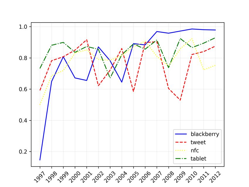
(a) TRI (b) SGNS
Figure 4: Time series based on TRI and SGNS of four words whose semantics
have changed between 2001-2013 according to the Oxford English Dictionary
(i.e., they have acquired a new meaning during this time period).
11TRI SGNS
Year Vocabulary Size File Size Vocabulary Size File Size
1996 454,751 284.9MB – –
1997 711,007 904.8MB – –
1998 704,453 823.3MB – –
1999 769,824 1.1GB – –
2000 847,318 1.5GB 235,428 114.7MB
2001 911,499 1.9GB 407,074 198.2MB
2002 945,565 2.1GB 571,419 277.8MB
2003 992,192 2.4GB 884,393 430.4MB
2004 1,040,470 2.7GB 1,270,804 619.1MB
2005 1,060,117 2.7GB 1,202,899 585.4MB
2006 1,076,523 2.7GB 1,007,582 490.6MB
2007 1,093,980 2.8GB 1,124,179 548.2MB
2008 1,105,511 2.9GB 1,173,870 572.2MB
2009 1,105,901 2.6GB 671,940 327.6MB
2010 1,125,201 2.8GB 1,183,907 576.8MB
2011 1,145,990 2.9GB 1,309,804 637.7MB
2012 1,144,764 3.0GB 1,607,272 784.0MB
2013 1,044,436 1.9GB 587,035 285.6MB
Table 2: Statistics about the vocabulary in terms of overall number of words
and (compressed) file size, per year and per method (TRI, SGNS).
the year 2000, according to the Oxford English Dictionary. Similarly, Figure 4
(b) shows the time series of the cosine distances of the same words that result
after Orthogonal Procrustes is applied on SGNS as described in Section 2.4.2.
In particular, we first align the embeddings matrices of a year T with respect
to the year 2000 and then we measure the cosine distance of the aligned word
vectors. As a result, this part of our dataset consists of 168,362 tokens and their
respective differences from the year 2000 during the years 2001-2013. We further
accompany these with the time series consisting of the number of occurrences
of each word in every year.
Figure 4 shows that the semantic similarity of the word “blackberry” de-
creases dramatically in 2004, which corresponds to the change point year de-
tected by the semantic change detection algorithm. On the other hand, Figure 4
(b) shows that the four words are moving away with time from their semantic
representation in the year 2000. We also find examples of cases of semantic
shifts corresponding to real-world events in SGNS representations: for example,
the meaning of the word “tweet” shifted more rapidly after Twitter’s foundation
(2006), whereas the lexical semantics of the word “tablet” mostly shifted in the
year 2010, at the time when the first mass-market tablet – iPad – was released.
Furthermore, as we showed in our previous work [4], it is possible to analyze
the neighborhood of a word (e.g. “blackberry”) in different years (e.g. in 2003
and 2004) in order to understand the semantic change it underwent. The list
12of neighborhoods can be computed as the most similar vectors in a given word
space. Similarly, in the case of SGNS we can measure the cosine similarity
between the word representations in different years.
3.4 Dataset Summary
Overall, our dataset consists of the following files:
• D-YEAR_merge_occ.gz: co-occurrences matrix for each year.
• YEAR.csv.zip: The SGNS word embeddings during the year YEAR, as de-
scribed in section 2.4.2. There are 14 files, one for each year between 2000
and 2013, and the size of each file is shown in Table 2.
• D-YEAR_merge.vectors.txt.gz: TRI embeddings for each year in tex-
tual format.
• D-YEAR_merge.vectors: TRI embeddings for each year in binary for-
mat. This vectors can be directly used with the TRI tool.10
• timeseries: four files containing the timeseries for the words based on
(a) their counts, as extracted from SGNS (count_timeseries.tsv), (b) the
cosine distances from their representations in the year 2000 based on
SGNS (w2v_dist_timeseries.tsv) and (c) the time series generated via
TRI-based pointwise and cumulative approaches (ukwac_all_point.csv,
ukwac_all_cum.csv respectively).
• vectors.elemental: TRI embeddings for the whole vocabulary in binary
format.
4 Technical Validation
We perform two sets of experiments in order to assess the quality of the em-
beddings generated via TRI and SGNS. In the first set, our goal is to measure
the embeddings’ ability to capture semantic properties of words, i.e. analogies,
similarities and relatedness levels. In the second set, we aim at exploring to
what extent the two types of contextual vectors capture the change in meaning
of words.
4.1 Static Tasks: Word-level Semantics
In this set of tasks we examine the ability of the word vectors to capture the
semantics of the words associated to them. We work on three different sub-tasks:
(a) word analogy, (b) word similarity and (c) word relatedness detection.
10 https://github.com/pippokill/tri
134.1.1 Tasks Description
Word Analogy Word analogy detection is the task of identifying relationships
between words in the form of “wa is to wb as wc is to wd ”, where wi is a word.
In our experiments, we make use of the widely employed dataset which was
created by Mikolov and colleagues [24] and which contains these relationships
in different categories:11
• Geography, e.g. Paris is to France as Madrid is to Spain.
• Currencies, e.g. Peso is to Argentina as euro is to Europe.
• Family, e.g. Boy is to girl as policeman is to policewoman.
• Grammar rules, e.g. Amazing is to amazingly as apparent is to apparently.
Given the vectors [va , vb , vc , vd ] of the words [wa , wb , wc , wd ] respectively, and
assuming an analogous relationship between the pairs [wa , wb ] and [wc , wd ] in
the form described above, previous work has demonstrated that in SGNS-based
embeddings, va − vb ≈ vc − vd . We perform this task by measuring the cosine
similarity sc that results when comparing the vector vc of the word wc against
the vector resulting from va − vb + vd . We apply this method to all the words in
the examples of the word analogy task set and we average across all examples.
Higher average cosine similarity scores indicate a better model.
TRI-based embeddings are not suitable for this kind of task due to the
nature of the vector space. TRI is not able to learn the linear dependency
between vectors in the space, which may be due to the Random Projection that
preserves all distance/similarity measures based on L2-norm, but it distorts the
original space and does not preserve the original position of vectors. We try
to simulate analogy by using vector orthogonalization as the negation operator
[43]. In particular, the vector sum vb + vd is orthogonalized with respect to the
vector va . For each word vector the cosine similarity is computed against the
vector obtained as the result of the orthogonalization, then the word with the
highest similarity is selected.
We perform experiments using our TRI and SNGS word vectors. For com-
parison purposes, we also employ the word2vec pre-trained embeddings gen-
erated in [24] as well as the GloVe embeddings released in [38]. These are
well-established sources of word vectors that have been trained on massive cor-
pora of textual data and have been employed in an extremely large body of
research work across multiple NLP tasks. In particular, for word2vec we employ
the 300-dimensional word vectors that were trained on Google news (prew2v )
[24], whereas for GloVe we use the 100-dimensional vectors trained on Twitter
(preglv ) [38]. As opposed to SGNS and TRI, prew2v and preglv are temporally
independent (i.e., there is one representation of each word through time). To
allow for a fair comparison, the analysis described here and in the following sec-
tions is on the intersected vocabulary across all years, i.e. on the set of words
occurring in all years in our corpus.
11 We list four categories, with one example for each of them.
14Word Similarity In the word similarity task, we are interested in detecting
the similarity between two words. We employ the dataset in [36], which contains
examples of 203 word pairs, along with their similarity score, as provided by two
annotators. We only use the 187 word pairs that consist of words present in
the intersected vocabulary, as before. We deploy the following experimental
setting: given the word vectors wa and wb of a pair of words, we measure their
cosine similarity sim(wa , wb ); subsequently, we measure the correlation between
sim(wa , wb ) and the ground truth. Higher values indicate a better model. We
compare performance against the baselines prew2v and preglv .
Word Relatedness Our final experiment in this section involves the task of
identifying the level of relatedness between two words. For example, the word
“computer” is much more closely related to the word “software” than to the
word “news”. We employ the word relatedness dataset introduced by [36], which
contains 252 examples of word pairs, along with their associated relatedness
score. As in the previous tasks, we only use the 232 examples that are present
in our intersected vocabulary; we deploy the same experimental setting as in
the case of the Word Similarity task and compare against the two previously
introduced baselines (prew2v , preglv ).
4.1.2 Results
Word Analogy The results are displayed in Figure 5. preglv outperforms
our models in almost all cases. SGN S achieves comparable performance to
preglv and prew2v , especially during the first years; comparably. T RI performs
poorly since it is not able to learn the linear dependency between vectors in
the space, which may be due to the Random Projection that preserves all dis-
tance/similarity measures based on L2-norm, but it distorts the original space
and does not preserve the original position of vectors. prew2v , preglv and SGN S
better capture relationships related to “Family” and “Grammar” than “Currency”
in our experiments.
Word Relatedness and Word Similarity Figure 6 shows the results on
the word similarity and word relatedness tasks. Here prew2v achieves the high-
est average Pearson correlation score across all years (.76 and .58 for the two
tasks, respectively). SGN S performs competitively (.57 vs .61, on average) and
outperforms in most cases (49. vs .45, on average) the preglv baseline for the
case of semantic similarity and relatedness, respectively. Importantly, its per-
formance is again consistent across time, ranging from .51 to .64 and from .42 to
.57 for the two respective tasks. TRI performs again more poorly and slightly
more inconsistently than SGN S, with its average (across years) evaluation score
ranging from .22 to .38 (average: .28) and from .08 to 0.29 (average: .22).
The results presented so far show that, overall, the SGN S and T RI em-
beddings do not outperform the two baselines (prew2v and preglv ) consisting of
static word representations in temporally independent tasks. This is partially
attributed to the facts that our resources are built on large-scale, yet potentially
15(a) Family (b) Grammar
(c) Geography (d) Currency
Figure 5: Results of the SGNS and TRI embeddings and the two baselines
models on the Word Analogy task.
(a) (b)
Figure 6: Results of the SGNS and TRI embeddings and the two baselines
models on the Word Similarity (a) and Word Relatedness (b) tasks.
16noisy content and are also restricted primarily to British English, which could
impose some geographical and linguistic biases. However, both representations
(SGN S, T RI) can be effectively utilised for a dynamic, i.e. temporally depen-
dent, task which cannot be dealt with static word representations, as we show
in the next section.
4.2 Dynamic Task: Semantic Change Detection
The major contribution of the T RI and SGN S embeddings of DUKweb consists
in their temporal dimension. To exploit this aspect, we measure their ability to
capture lexical semantic change over time.
Experimental Setting We use as ground truth 65 words that have changed
their meaning between 2001 and 2013 according to the Oxford English Dic-
tionary [40]. We define the task in a time sensitive manner: given the word
representations in the year 2000 and in the year X, our aim is to find the words
whose lexical semantics have changed the most. We vary X from 2001 to 2013,
so that we get clearer insights on the effectiveness of the word representations.
Since our ground truth consists of words that are present in the OED, we also
limit our analysis to the 47,834 words that are present both in the OED and in
the TRI/SGNS vocabularies.
Models We employ four variants of Orthogonal Procrustes-based methods
operating on SGN S from our prior work [40, 41] and two models operating on
T RI, as follows:
• SGN Spr employs the Orthogonal Procrustes (OP) alignment to align the
word representations in the year X based on those for the year 2000;
• SGN Spr(a) applies OP in two passes: during the first pass, it selects the
most stable (“anchor”) words (i.e., those whose aligned representations
across years have the highest cosine similarity); then, it learns the align-
ment between the representations in the years 2000 and X using solely
the anchor words;
• SGN Spr(d) applies OP in several passes executed in two rounds: during
the first round, it selects the most stable (“diachronic anchor”) words
across the full time interval; then, it learns the alignment between the
representations in the years 2000 and X using solely the diahcronic anchor
words;
• T RIc and T RIp exploit time-series built by the cumulative and point-wise
approach, respectively (see Section 2.4.1)
17Evaluation In all of the SGN S models, we rank the words on the basis of
the cosine similarity of their representations in the aligned space, such that
words in the higher ranks are those whose lexical semantics has changed the
most. For the T RI-based models, the Mean Shift algorithm [27] is used for
detecting change points in the time series consisting of the cosine similarity
scores between the representations of the same word in each year covered by the
corpus. For each detected change point, a p-value is estimated according to the
confidence level obtained by the bootstrapping approach proposed in [27], then
words are ranked according to the p-value in ascending order. Finally, we run
the evaluation using the recall at 10% of the size of the dataset as well as the
average rank (µr , scaled in [0,1]) of the 65 words with altered semantics. Higher
recall-at-k and lower µr scores indicate a better performance.
Results Tables 3 and 4 present the results of our models in terms of µr and
recall-at-k, respectively. In both cases, the SGN S-based approaches perform
better than T RI: on average, the best-performing SGNS-based model achieves
27.42 in µr (SGNSpr(a) ) and 29.59 in recall-at-k (SGN Spr ). The difference
compared to TRI is attributed to their ability to better capture the contex-
tualised representation of the words in our corpus. Nevertheless, TRI has re-
cently achieved state-of-the-art performance on semantic change detection in
the Swedish language [39]. Furthermore, despite their superior performance in
this task, the Procrustes- and SGNS-based approaches have the shortcoming
that they operate on a common vocabulary across different years; thus, words
that have appeared at a certain year cannot be detected in these variants – a
drawback is not present in the case of TRI.
Finally, we inspect the semantically altered words that have been detected
by each model. Table 3 displays the most “obvious” and challenging examples
of semantic change, as ranked on a per-model basis. It becomes evident that
the two different word representations better capture the changes of different
words. This is attributed to the different nature of the two released word repre-
sentations. Incorporating hybrid approaches operating on multiple embedding
models could be an important direction for future work in this task.
Usage Notes
The DUKweb datasets can be used for various time-independent tasks, as demon-
strated in this article. Their major application is for studying how word mean-
ing changes over time (i.e., semantic change) in a computational and linguistic
context. The instructions on how to run our code for the experiments as well
as for further downstream tasks have been made publicly available (see Code
Availability).
18SGNSpr SGNSpr(a) SGNSpr(d) TRIc TRIp
cloud sars eris tweet root
sars fap ds qe purple
tweet trending follow parmesan blackberry
trending eris blw event tweet
fap tweet fap sup follow
tweeter preloading unlike status eta
like chugging chugging grime prep
preloading bloatware roasting prep grime
bloatware tweeter even trending status
parmesan parmesan parmesan tomahawk tomahawk
Table 3: Examples of easy-to-predict (top-5) and hard-to-predict (bottom-5)
words by our SNGS and TRI models.
Model 2001 2002 2003 2004 2005 2006 2007 2008 2009 2010 2011 2012 2013
SGNSpr 36.33 34.03 30.90 26.85 29.29 27.16 26.88 28.60 25.16 27.21 25.69 25.83 29.13
SGNSpr(a) 36.83 32.30 31.67 27.23 27.27 26.31 25.25 28.15 26.54 27.14 27.59 30.42 28.78
SGNSpr(d) 33.09 28.32 28.91 23.17 25.13 27.99 30.38 25.60 27.17 28.96 25.08 27.84 24.83
TRIc 54.65 51.22 56.64 55.63 50.90 55.98 60.96 58.03 58.94 56.59 59.00 45.96 45.72
TRIp 56.77 59.79 54.81 54.61 53.22 54.39 55.44 55.12 59.76 59.22 53.22 46.30 50.07
Table 4: Average rank of a semantically shifted word; lower scores indicate a
better model.
Model 2001 2002 2003 2004 2005 2006 2007 2008 2009 2010 2011 2012 2013
SGNSpr 16.92 23.08 21.54 26.15 35.38 30.77 29.23 32.31 38.46 29.23 32.31 36.92 32.31
SGNSpr(a) 15.38 24.62 23.08 23.08 30.77 35.38 29.23 32.31 33.85 32.31 33.85 26.15 32.31
SGNSpr(d) 15.38 18.46 27.69 29.23 35.38 23.08 27.69 36.92 30.77 23.08 35.38 18.46 33.85
TRIc 7.69 12.31 6.15 3.08 12.31 7.69 7.69 7.69 6.15 7.69 4.62 13.85 12.31
TRIp 12.31 4.62 7.69 10.77 10.77 4.62 13.85 7.69 3.08 4.62 12.31 21.54 13.85
Table 5: Recall at 10% of our different SGNS and TRI models.
19Code Availability
The creation of the described datasets requires several steps, each step is per-
formed by a different software. All the software is freely available, in particular:
• the code for the processing of the JISC UK Web Domain Dataset for pro-
ducing both the WET and tokenized files: https://github.com/alan-
turing-institute/UKWebArchive_semantic_change;
• the software for building both co-occurrences matrices and TRI: https:
//github.com/alan-turing-institute/temporal-random-indexing;
• the code for the experiments conducted in section 4 can be found at https:
//github.com/alan-turing-institute/DUKweb
For information on our input data, refer to: https://data.webarchive.org.
uk/opendata/ukwa.ds.2/
Acknowledgements
This work was supported by The Alan Turing Institute under the EPSRC grant
EP/N510129/1 and the seed funding grant SF099.
Author contributions
A.T. conducted the experiments for the SGNS embeddings and wrote sections
2.4.2, 3.2, 3.3 and 4. P.B. conducted the experiments for the TRI embed-
dings and contributed to sections 1, 2.1, 2.2, 2.3, 2.4.1, 3.1, 3.3, 3.4. M.B.
co-supervised this work, contributed to the design of the experiments and con-
tributed to subsection 2.4.2. M.C. co-supervised this work, contributed to the
design of the experiments and contributed to subsection 2.4.2. B.McG. was the
main supervisor of this work, contributed to the design of the experiments and
wrote section 1. All authors reviewed and approved the final manuscript.
Competing interests
The authors declare no competing interests.
References
[1] M. Chinazzi, B. Gonçalves, Q. Zhang, and Alessandro Vespignani. 2019.
Mapping the physics research space: a machine learning approach. EPJ
Data Science, 8.
20[2] Basile, P., Caputo, A., Semeraro, G.: Analysing word meaning over time by
exploiting temporal random indexing. In: R. Basili, A. Lenci, B. Magnini
(eds.) First Italian Conference on Computational Linguistics CLiC-it 2014.
Pisa University Press (2014)
[3] Basile, P., Caputo, A., Semeraro, G.: Temporal random indexing: A system
for analysing word meaning over time. Italian Journal of Computational
Linguistics 1(1), 55–68 (2015)
[4] Basile, P., McGillivray, B.: Discovery Science, Lecture Notes in Computer
Science, vol. 11198, chap. Exploiting the Web for Semantic Change Detec-
tion. Springer-Verlag (2018)
[5] Bojanowski, P., Grave, E., Joulin, A., Mikolov, T.: Enriching word vectors
with subword information. arXiv preprint arXiv:1607.04606 (2016)
[6] Cieliebak, M., Deriu, J., Uzdilli, F., Egger, D.: A Twitter Corpus and Bench-
mark Resources for German Sentiment Analysis. In: Proceedings of the 4th
International Workshop on Natural Language Processing for Social Media
(SocialNLP 2017). Valencia, Spain (2017)
[7] Efron, B., Tibshirani, R.J.: An introduction to the bootstrap. Chapman
and Hall/CRC (1994)
[8] Firth, J.R.: Papers in Linguistics 1934–1951. Oxford University Press (1957)
[9] Garg, N., Schiebinger, L., Jurafsky, D., Zou, J.: Word Embeddings Quantify
100 Years of Gender and Ethnic Stereotypes. PNAS 115 (2017). URL
http://arxiv.org/abs/1711.08412
[10] Google Books Ngram Viewer (2010) URL http://storage.googleapis.
com/books/ngrams/books/datasetsv2.html
[11] Grayson, S., Mulvany, M., Wade, K., Meaney, G., Greene, D.: Novel2Vec:
Characterising 19th Century Fiction via Word Embeddings. In: 24th Irish
Conference on Artificial Intelligence and Cognitive Science (AICS’16), Uni-
versity College Dublin, Dublin, Ireland, 20-21 September 2016 (2016)
[12] Hamilton, W.L., Leskovec, J., Jurafsky, D.: Cultural shift or linguistic
drift? comparing two computational measures of semantic change. In:
Proceedings of the 2016 Conference on Empirical Methods in Natural Lan-
guage Processing, pp. 2116–2121. Association for Computational Linguistics
(2016). 10.18653/v1/D16-1229. URL http://aclweb.org/anthology/
D16-1229
[13] Hamilton, W.L., Leskovec, J., Jurafsky, D.: Diachronic word embeddings
reveal statistical laws of semantic change. Proceedings of the 54th Annual
Meeting of the Association for Computational Linguistics (2016)
21[14] Hamilton, W.L., Leskovec, J., Jurafsky, D.: HistWords: Word Embeddings
for Historical Text (2016) URL https://nlp.stanford.edu/projects/
histwords/
[15] Hellrich, J., Hahn, U.: Exploring Diachronic Lexical Semantics with J E
S EM E. In: Proceedings of ACL 2017, System Demonstrations, pp. 31–36
(2017). URL http://aclweb.org/anthology/P17-4006
[16] JISC, the Internet Archive: Jisc uk web domain dataset (1996-2013) (2013).
https://doi.org/10.5259/ukwa.ds.2/1
[17] Heuser, R.: Word2Vec Models for Twenty-year Periods of 18C
(ECCO, “Literature and Language”) Internet Archive (2016) URL
https://archive.org/details/word-vectors-18c-word2vec-models-
across-20-year-periods
[18] Kim, Y., Chiu, Y.I., Hanaki, K., Hegde, D., Petrov, S.: Temporal Analysis
of Language through Neural Language Models. Arxiv pp. 61–65 (2014).
URL http://arxiv.org/abs/1405.3515
[19] Kulkarni, V., Al-Rfou, R., Perozzi, B., Skiena, S.: Statistically significant
detection of linguistic change. In: Proceedings of the 24th International
Conference on World Wide Web, pp. 625–635. ACM (2015)
[20] Andrey Kutuzov, Lilja Øvrelid, Terrence Szymanski, and Erik Velldal.
2018. Diachronic word embeddings and semantic shifts: A survey. In Pro-
ceedings of the 27th International Conference on Computational Linguistics,
pages 1384–1397, Santa Fe, New Mexico, USA. Association for Computa-
tional Linguistics.
[21] Lenci, A.: Distributional semantics in linguistic and cognitive research.
Italian journal of linguistics 20(1), 1–31 (2008)
[22] Lin, Y., Michel, J.-B., Aiden Lieberman, E., Orwant, J., Brockman, W.,
Petrov, S.: Syntactic annotations for the Google Books Ngram corpus. In:
Proceegins of ACL, System Demonstrations, 169–174 (2012)
[23] Mikolov, T., Chen, K., Corrado, G., Dean, J.: Efficient estimation of word
representations in vector space. In: Proceedings of Workshop at the Inter-
national Conference on Learning Representations (ICLR) (2013)
[24] Mikolov, T., Sutskever, I., Chen, K., Corrado, G. S. and Dean, J. Dis-
tributed representations of words and phrases and their compositionality. In
Advances in Neural Information Processing systems 26, 3111–3119 (NIPS,
2013).
[25] Mitchell, J., Lapata, M.: Composition in distributional models of seman-
tics. Cognitive Science 34(8), 1388–1429 (2010)
22[26] Nina Tahmasebi, Lars Borin, and Adam Jatowt. 2018. Survey of compu-
tational approaches to lexical semantic change. In Preprint at ArXiv 2018.
[27] Taylor, W.A.: Change-point analysis: a powerful new tool for detecting
changes. Taylor Enterprises, Inc. (2000)
[28] Zhang, Y., Chen, Q., Yang, Z. et al. BioWordVec, improving biomedical
word embeddings with subword information and MeSH. Scientific Data 6,
52 (2019). https://doi.org/10.1038/s41597-019-0055-0
[29] Schönemann, Peter H., A generalized solution of the orthogonal procrustes
problem. Psychometrika 31(1), 1–10 (1966)
[30] Conneau, Alexis and Lample, Guillaume and Ranzato, Marc’Aurelio and
Denoyer, Ludovic and Jégou, Hervé, Word translation without parallel data.
arXiv:1710.04087 (2017)
[31] Ruder, Sebastian and Cotterell, Ryan and Kementchedjhieva, Yova and Sø-
gaard, Anders, A Discriminative Latent-Variable Model for Bilingual Lexi-
con Induction. Proceedings of the 2018 Conference on Empirical Methods
in Natural Language Processing,458–468 (2018)
[32] Shoemark, Philippa and Liza, Farhana Ferdousi and Nguyen, Dong and
Hale, Scott and McGillivray, Barbara, Room to Glo: A systematic compar-
ison of semantic change detection approaches with word embeddings, Pro-
ceedings of the 2019 Conference on Empirical Methods in Natural Language
Processing and the 9th International Joint Conference on Natural Language
Processing (EMNLP-IJCNLP), 66–76 (2019)
[33] Shoemark, Philippa and Ferdousi Liza, Farhana and Hale, Scott A.
and Nguyen, Dong and McGillivray, Barbara. Monthly word embed-
dings for Twitter random sample (English, 2012-2018) [Data set], Pro-
ceedings of the 2019 Conference on Empirical Methods in Natural Lan-
guage Processing and the 9th International Joint Conference on Nat-
ural Language Processing (EMNLP-IJCNLP). Hong Kong: Zenodo.
http://doi.org/10.5281/zenodo.3527983 (2019)
[34] Schlechtweg, Dominik and Hatty, Anna and del Tredici, Marco and Schulte
im Walde, Sabine, A Wind of Change: Detecting and Evaluating Lexical Se-
mantic Change across Times and Domains, Proceedings of the 57th Annual
Meeting of the Association for Computational Linguistics (ACL), 732–746
(2019)
[35] Tsakalidis, Adam and Bazzi, Marya and Cucuringu, Mihai and Basile, Pier-
paolo and McGillivray, Barbara, Mining the UK Web Archive for Semantic
Change Detection, Proceedings of the International Conference on Recent
Advances in Natural Language Processing (RANLP), 1212–1221 (2019).
23[36] Agirre, Eneko and Alfonseca, Enrique and Hall, Keith and Kravalova, Jana
and Pasca, Marius and Soroa, Aitor, A Study on Similarity and Relatedness
Using Distributional and WordNet-based Approaches, Proceedings of the
International Conference on North American Chapter of the Association for
Computational Linguistics (NAACL-HLT), 19–27 (2009).
[37] Pumir, Thomas and Singer, Amit and Boumal, Nicolas, The generalized
orthogonal Procrustes problem in the high noise regime, arXiv: 1907.01145
(2019).
[38] Pennington, Jeffrey and Socher, Richard and Manning, Christopher D.,
Glove: Global vectors for word representation, Proceedings of the 2014 Con-
ference on Empirical Methods in Natural Language Processing (EMNLP),
1532–1543 (2014).
[39] Schlechtweg, Dominik and McGillivray, Barbara and Hengchen, Simon and
Dubossarsky, Haim and Tahmasebi, Nina: SemEval-2020 Task 1: Unsuper-
vised Lexical Semantic Change Detection, Proceedings of the 14th Interna-
tional Workshop on Semantic Evaluation (2020)
[40] Tsakalidis, Adam and Bazzi, Marya and Cucuringu, Mihai and Basile, Pier-
paolo and McGillivray, Barbara: Mining the UK Web Archive for Semantic
Change Detection, Proceedings of Recent Advances in Natural Language
Processing (RANLP) (2019)
[41] Tsakalidis, Adam and Liakata, Maria: Sequential Modelling of the Evolu-
tion of Word Representations for Semantic Change Detection, Proceedings of
the 2020 Conference on Empirical Methods in Natural Language Processing
(EMNLP) (2020)
[42] Basile, Pierpaolo and Caputo, Annalina and Caselli, Tommaso and Cas-
sotti, Pierluigi and Varvara, Rossella: Overview of the EVALITA 2020 Di-
achronic Lexical Semantics (DIACR-Ita) Task, Proceedings of the 7th evalu-
ation campaign of Natural Language Processing and Speech tools for Italian
(EVALITA) (2020)
[43] Widdows, D.: Orthogonal negation in vector spaces for modelling word-
meanings and document retrieval, Proceedings of the 41st annual meeting
of the association for computational linguistics (2003)
[44] Zhao, Zhe and Liu, Tao and Li, Shen and Li, Bofang and Du, Xiaoy-
ong: Ngram2vec: Learning improved word representations from ngram co-
occurrence statistics, Proceedings of the 2017 conference on empirical meth-
ods in natural language processing (2017)
[45] Levy, Omer and Goldberg, Yoav: Dependency-based word embeddings,
Proceedings of the 52nd Annual Meeting of the Association for Computa-
tional Linguistics (ACL) (2014)
24You can also read