Efficient experimental quantum fingerprinting with channel multiplexing and simultaneous detection - Nature
←
→
Page content transcription
If your browser does not render page correctly, please read the page content below
ARTICLE
                  https://doi.org/10.1038/s41467-021-24745-x                 OPEN

                  Efficient experimental quantum fingerprinting with
                  channel multiplexing and simultaneous detection
                  Xiaoqing Zhong            1 ✉,   Feihu Xu       2,   Hoi-Kwong Lo1,3,4 & Li Qian               3

                  Quantum communication complexity explores the minimum amount of communication
                  required to achieve certain tasks using quantum states. One representative example is
1234567890():,;

                  quantum fingerprinting, in which the minimum amount of communication could be expo-
                  nentially smaller than the classical fingerprinting. Here, we propose a quantum fingerprinting
                  protocol where coherent states and channel multiplexing are used, with simultaneous
                  detection of signals carried by multiple channels. Compared with an existing coherent
                  quantum fingerprinting protocol, our protocol could consistently reduce communication time
                  and the amount of communication by orders of magnitude by increasing the number of
                  channels. Our proposed protocol can even beat the classical limit without using
                  superconducting-nanowire single photon detectors. We also report a proof-of-concept
                  experimental demonstration with six wavelength channels to validate the advantage of our
                  protocol in the amount of communication. The experimental results clearly prove that our
                  protocol not only surpasses the best-known classical protocol, but also remarkably outper-
                  forms the existing coherent quantum fingerprinting protocol.

                  1 Center for Quantum Information and Quantum Control, Dept. of Physics, University of Toronto, Toronto, Ontario, Canada. 2 Hefei National Laboratory for

                  Physical Sciences at the Microscale and Department of Modern Physics, University of Science and Technology of China, Hefei, China. 3 Center for Quantum
                  Information and Quantum Control, Dept. of Electrical & Computer Engineering, University of Toronto, Toronto, Ontario, Canada. 4 Department of Physics,
                  University of Hong Kong, Hong Kong, China. ✉email: xzhong@physics.utoronto.ca

                  NATURE COMMUNICATIONS | (2021)12:4464 | https://doi.org/10.1038/s41467-021-24745-x | www.nature.com/naturecommunications                              1
ARTICLE                                                                 NATURE COMMUNICATIONS | https://doi.org/10.1038/s41467-021-24745-x

Q
         uantum communication is the study of information-                   number of the fingerprint in this coherent quantum fingerprinting
         transmission tasks that can be facilitated by using                 (CQF) protocol is μ. Therefore, for CQF protocol with a fixed μ,
         quantum mechanical systems1. The power of quantum                   the minimum amount of communication can still be exponentially
mechanics enables quantum communication to perform tasks                     smaller than the classical fingerprinting protocol. Refs. 30,31 have
that could not be accomplished in a classical system. One of the             successfully demonstrated the proof-of-principle experiment of
best-known examples is quantum cryptography that enables                     CQF protocol and prove that less information is communicated in
information-theoretically secure communication between two                   the CQF system compared with the best-known classical
parties that share random keys through quantum key dis-                      protocol25. Nonetheless, this CQF protocol uses a number of
tribution (QKD)2–6. Apart from quantum cryptography,                         optical modes that is proportional to the input size n, hence the
quantum communication complexity (QCC)7–10 is another                        communication time is quadratically increased compared with the
important example that shows quantum superiority over its                    classical system30,31. In addition, the minimum amount of com-
classical counterpart–classical communication complexity11–14.               munication in CQF protocol has a dependence on μ, a value that
In the basic model of communication complexity13, Alice and                  has a lower limit due to experimental imperfections29, among
Bob each is given an n-bit string x and y, respectively. The                 which the dark counts from the single-photon detector (SPD)
classical communication complexity exploits the minimum                      (used for Charlie’s detection) are a dominant factor30. As indi-
amount of communication necessary among participants,                        cated in ref. 31 where superconducting-nanowire single-photon
namely the minimum number of bits of communication, such                     detectors (SNSPD) with very low dark count rates (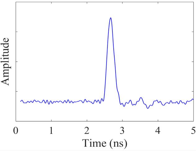
NATURE COMMUNICATIONS | https://doi.org/10.1038/s41467-021-24745-x                                                                         ARTICLE

                                                                          Charlie

                                         …                                                                       …

                                 ( )               …                                                        …               ( )

                                       ( )                                                                            ( )

                                              ( )                                                               ( )
                                                       Alice                                      Bob
                                             ( )                                                                            ( )

Fig. 1 Theoretical scheme of coherent quantum fingerprinting with wavelength-division multiplexing. Alice (Bob) applies error-correction code to her
(his) input x(y) and obtains E(x)(E(y)). Then she (he) divides E(x)(E(y)) into k subcodewords and prepares the corresponding subfingerprints Ej(x)(Ej(y)) in
k-different wavelength channels. The k subfingerprints are multiplexed into one single-mode fiber through a multiplexer (MUX) and sent to Charlie’s beam
splitter. On Charlie’s station, demultiplexing is not required. The k pairs of pulses interfere simultaneously and share a pair of single-photon detectors D0
and D1. Charlie records the total counts at D0 and D1, based on which Charlie determines whether the inputs are the same or different.

Result                                                                          subfingerprint consists of m/k-coherent states and is described as
WDM–CQF protocol. In the CQF protocol29, Alice first prepares
                                                                                                          m=k
her coherent fingerprint jαiA as                                                                                  Ej ðxÞi α
                                                                                                 jαiA;j ¼  ð1Þ        pffiffiffiffi :              ð4Þ
                                                                                                          i¼1              m i

                                m  EðxÞi α                                     Ej(x)i is the ith bit of the jth subcodeword Ej(x) (j ∈ [1, k]).

                      jαiA ¼  ð1Þ     pffiffiffiffi :                         ð2Þ
                             i¼1           m           i
                                                                                Figure 1 shows the schematic set-up of the WDM–CQF protocol.
                                                                                As shown in Fig. 1, Alice and Bob assign each subfingerprint to a
Bob’s fingerprint jαiB has the same expression as Eq. (2) with                   wavelength channel and multiplex the k-wavelength channels into
changing subscript A into B and changing input x into y. The m-                 a single optical channel. Then they send their fingerprints to
bit strings E(x) and E(y) are the codewords of Alice and Bob,                   Charlie for detection through the optical channels. In total, m/k-
respectively, obtained by applying error-correction code (ECC) to               wavelength-composite pulses are sent from Alice/Bob to Charlie.
the n-bit input strings x and y. The ECC has a code rate c (¼ mn
ARTICLE NATURE COMMUNICATIONS | https://doi.org/10.1038/s41467-021-24745-x
SPD, would also give clicks in D1 even when the inputs are the However, SNSPDs are much more expensive than the regular
same. Here we adopt the decision mechanism introduced in SPDs and require very low temperature. Instead of using SNSPDs
ref. 30. In ref. 30, for the equal and different inputs cases, photon to decrease Pdark, our WDM–CQF protocol simply increases
counts at detector D1 have the binomial distributions B(m, PE), the signal probability PE/D,signal in Eq. (6) and Eq. (7) by
and B(m, PD) respectively. PE and PD are the probabilities of D1 simultaneously detecting k pairs of wavelength components.
obtaining a click in a single-detection window. Based on these Because a low value of μ is preferred in the protocol, most of the
distributions, a threshold C1,th is chosen. Charlie then compares coherent states are empty when they arrive at Charlie’s station.
the total counts at D1 with C1,th. If the total counts are The signal probability PE/D,signal primarily comes from the
smaller than C1,th, Charlie concludes that the inputs are equal. photons in one-wavelength component. With a reasonable
Otherwise, Charlie concludes that the inputs are different. In our number of wavelength channels (say 1 ≤ k ≤ 1000), the probability
WDM–CQF system, since each detection event is independent, of more than one-wavelength component containing photons
the photon counts at D1 also have the binomial distributions B when arriving at Charlie’s station is so low (even lower than Pdark)
(M, PE) and B(M, PD). Note that m is replaced by M, since that we can simply ignore the multi-wavelength contributions to
in total, M-wavelength-composite pulses are sent from Alice/Bob the detection event (detailed analysis can be found in Methods)
to Charlie in the WDM–CQF protocol. The amplitude of each Moreover, the information of which wavelength component
pulse is carries a photon is not important and only the total counts
μ μ detected on D1 are valued. Therefore, demultiplexing is not
¼ : ð5Þ necessary on Charlie’s station. k pairs of coherent states at
m=k M
different wavelengths interfere simultaneously and are detected
The detection probabilities PE and PD are by a single pair of detectors in each detection window. Compared
2μη with the single-wavelength CQF protocol, the signal probability
PE ¼ PE;signal þ Pdark ¼ ð1 νÞð1 e M Þ þ Pdark ; ð6Þ
PE/D,signal is increased without changing μ and the error Perror is
then decreased. Therefore, to achieve the same tolerable error
PD ¼ PD;signal þ Pdark probability ϵ, our WDM–CQF protocol requires a lower value of
ð7Þ
2μη
¼ ðδν þ ð1 δÞð1 νÞÞð1 e M Þ þ Pdark : μ than the single-wavelength CQF protocol. Consequently, as
indicated in Eq. (3), less amount of communication is required in
For the probability PD, we assume the worst-case scenario that our WDM–CQF protocol than the single-wavelength CQF
the codewords E(x) and E(y) have the minimum distance. ν is the protocol. More wavelength channels are used, less μ is needed,
interference visibility that considers the imperfect interference and greater gain of the amount of communication is obtained by
due to various factors. For example, the interfering states from our protocol.
Alice and Bob might not arrive at Charlie’s station simulta- Figure 2 shows the amount of communication between Alice/
neously. Their polarization states might not be exactly the same Bob and Charlie over 0 km, 40 km, and 80 km fibers in different
after traveling a long distance and the phase drift could also be fingerprinting protocols as a function of the input size n. Note
different. To maximize ν, one must minimize these mismatches. η that the distance considered in the work is the total length of
is the optical channel transmittance. Here we consider that the fibers that connect between Alice and Charlie and fibers that
optical channel loss between Alice and Charlie is the same as the connect between Bob and Charlie. In short, we just call it the
loss between Bob and Charlie, i.e., ηA = ηB = η. If the channel overall distance between Alice and Bob. In this log–log plot,
losses are different, Alice and Bob simply use different signal practical experimental parameters are considered. The interfer-
intensities μA and μB such that μA × ηA = μB × ηB. If the detector’s ence visibility is assumed to be 97%. The dark-count rate and the
efficiency ηdec is taken into consideration, then η = ηA/B × ηdec. detector’s efficiency are 100 Hz and 25%, respectively. (We use
Pdark is the dark-count probability per detection gate of the SPDs. the parameters from the best available commercial SPD ID230
The error probability for this decision mechanism is from ID Quantique to show the best performance of our
Perror ¼ max½PðC1;E > C1;th Þ; PðC 1;D < C1;th Þ; ð8Þ protocol.) The detection window is 500 ps. The tolerable error
probability is chosen to be ϵ = 10−5. The input size n varies from
and it should be smaller than the tolerable probability ϵ. C1,E and 105 to 1018. (Details about the simulation are discussed in
C1,D are the detected total counts at detector D1 for the equal and Methods.) As shown in Fig. 2, for different distances, all the
different input cases, respectively. For each input size n, the WDM–CQF protocols require less communication than the best-
choice of threshold C1,th depends on the total mean photon known classical fingerprinting protocol. As k gets larger, the
number μ. As indicated in Eq. (6) and Eq. (7), when μ is so small advantage of WDM–CQF protocol is more evident. Compared
such that PE/D,signal ≪ Pdark, the probabilities PE and PD are with the original CQF protocol (k = 1), our WDM–CQF protocol
dominated by Pdark and the distributions B(m/k, PE) and B(m/k, with k≥100 reduces the amount of communication by at least one
PD) are fairly close to each other. Consequently, the error order of magnitude. In fact, with the parameters used in this
probability would be very large. Therefore, a large value of μ is simulation, the original CQF protocol (k = 1) cannot beat the
preferred for minimizing the error probability. However, as classical limit even when the overall distance between Alice and
mentioned before, the amount of communication required by the Bob is 0 km. However, with only k = 10 wavelength channels
coherent fingerprint is proportional to the mean photon number applied, our WDM–CQF protocol can transmit less information
μ. So, for each input size n, one has to balance the two demands than the classical limit for 0 km. When the distance increases,
of low error probability and a small amount of communication. more photons are needed to compensate the channel loss. Hence,
That is to say, one has to find the minimum μ (and its the amount of communication in the coherent fingerprinting
corresponding threshold C1,th), which gives the error probability system increases with the channel distance. But, in our
Perror smaller than ϵ. More details about the optimization of μ can WDM–CQF protocol, the channel loss can be compensated by
be found in “Method”. adding wavelength channels. Therefore, even when the distance
It is straightforward to think that the lower the dark-count increases, our WDM–CQF protocol can always beat the classical
probability Pdark is, the smaller μ can be found. Ref. 31 uses limit without using SNSPDs, as depicted in Fig. 2. Remarkably,
SNSPDs with ultralow dark count rate (0.11 Hz) significantly when the overall distance between Alice and Bob is 40 km, our
reduces the value of μ, hence, it can beat the classical limit. WDM–CQF protocol requires around 100-wavelength channels
4 NATURE COMMUNICATIONS | (2021)12:4464 | https://doi.org/10.1038/s41467-021-24745-x | www.nature.com/naturecommunicationsNATURE COMMUNICATIONS | https://doi.org/10.1038/s41467-021-24745-x ARTICLE
Amount of communication
Amount of communication
0 km 40 km
1010 1010
5
105 10
10 15
10 10 1015 10 10
Input size n Input size n
Amount of communication
10 80 km
10
Classical protocol
Classical limit
WDM-CQF (k=1)
WDM-CQF (k=10)
WDM-CQF (k=100)
5
10 WDM-CQF (k=1000)
10 15
10 10
Input size n
Fig. 2 Log–log plot of the simulation results of the amount of communication required in different fingerprinting protocols as a function of input size n
for three distances, 0 km, 40 km, and 80 km. The solid red line represents the best-known classical fingerprinting protocol25. The solid black line
represents the classical limit introduced in31. The dash curves are to the simulation results of coherent quantum fingerprinting (CQF) protocol with
wavelength-division multiplexing (WDM). Different values of k correspond to a different number of wavelength channels. When k = 1, the scheme
becomes the original CQF protocol. In the simulation, we use parameters achievable with single-photon avalanche diodes, with a dark-count rate of 100 Hz
and 25% detector efficiency. The interference visibility is assumed to be 97% and the detection window is 500 ps. The applied error-correction code has a
code rate c = 0.2398 and δ = 0.22. The total mean photon number μ for each n and k is optimized to fulfill the condition Perror < ϵ = 10−5.
to beat the limit. We remark that it is currently feasible to achieve
around 100 simultaneous channels by using WDM, since there Lasers
PC MUX
have been many reports of classical transmission experiments
with WDM over more than 100 channels37,38. Moreover, the total Pol
IMC D0
cost of adding wavelength channels is much lower compared with ATT
applying SNSPDs. When the distance is longer, more channels BS D1
are required by our WDM–CQF protocol to beat the classical
limit. The implementation of WDM–CQF with a large number of Alice Bob
wavelength channels is very challenging. To circumvent this issue, PC PC
PC PC
one can combine other multiplexing schemes with wavelength SMF SMF
multiplexing to reduce the number of wavelength channels. For PMA DCF PMB
example, one can use time-division multiplexing (TDM), i.e., use PC PC
fast modulators to add more temporal channels within one
detection window. We would like to emphasize that our
Fig. 3 Schematic experimental set-up of coherent quantum fingerprinting
WDM–CQF protocol takes the advantage of the simultaneous
with wavelength-division multiplexing. Six continuous-wave lasers are
detection of many bits of information within one detection
located on Charlie’s side with wavelength ranging from 1542.9 nm to
window. These bits of information can be distributed in, but not
1554.9 nm, equally spaced by δλ = 2.4 nm. Photons coming out the lasers
confined to the wavelength channels.
are multiplexed through a multiplexer (Mux) into a single-mode fiber and
pass through a polarizer (Pol). An intensity modulator (IM) and an optical
Experimental set-up. In this section, we show a proof-of-concept variable attenuator are used to create weak coherent pulses. The pulses
experimental demonstration of our WDM–CQF protocol. Six- then enter the loop through a circulator (C) and a beam splitter (BS) and
wavelength channels are used and a two-way quantum commu- travel to Alice/Bob through 20 km single-mode fibers (SMF). Alice and Bob
nication system consisting of a Sagnac interferometer is are separated by another 6.9 km of compensation-dispersion fibers (DCF).
employed. This system configuration is similar to that of a twin- On Alice’s (Bob’s) station, the phase modulator (PM) is on only when the
field QKD system39. The Sagnac arrangement is chosen to pro- clockwise (counterclockwise) traveling pulses arrive and the phase
vide a phase reference between Alice and Bob. Moreover, the information is added to the pulses accordingly. After the phase modulation,
common path feature of Sagnac interferometer automatically the clockwise and counterclockwise traveling pulses go back to Charlie and
stabilizes the phase fluctuation along the optical channel and interfere with each other at Charlie’s beam splitter. The results are recorded
ensures that two beams emerge at the beam splitter simulta- by two single-photon detectors D0 and D1. Polarization controllers (PC) are
neously. The schematic experimental set-up is shown in Fig. 3. designed for the polarization alignment for the beams in six-wavelength
On Charlie’s station, the continuous waves (cw) coming out of six channels.
NATURE COMMUNICATIONS | (2021)12:4464 | https://doi.org/10.1038/s41467-021-24745-x | www.nature.com/naturecommunications 5ARTICLE NATURE COMMUNICATIONS | https://doi.org/10.1038/s41467-021-24745-x
(a) (b)
Amplitude
Amplitude
…
Time (ns) Time (ns)
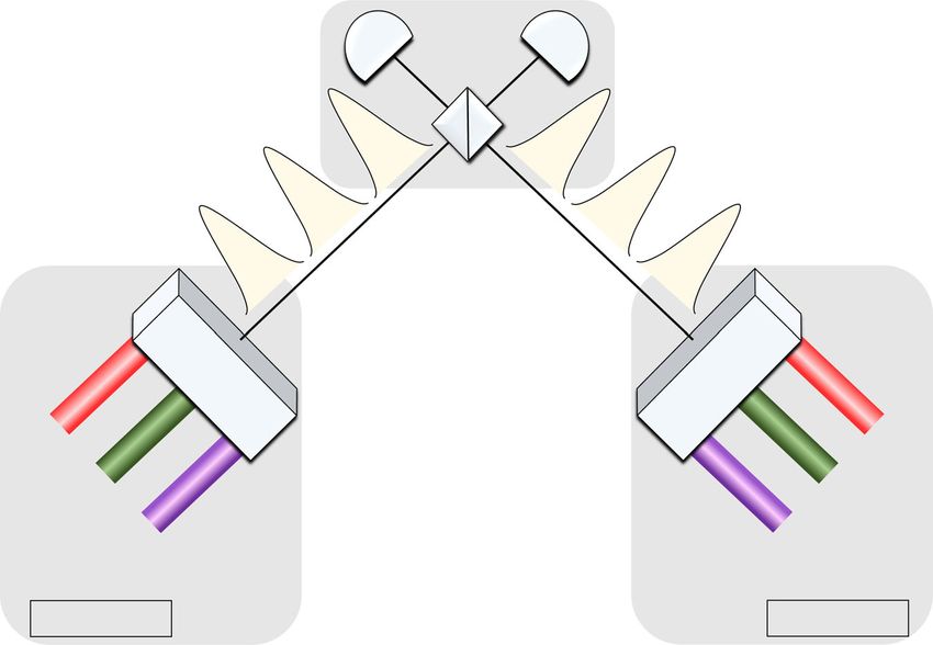
Fig. 4 Arrival times of different wavelength components. The wavelength components traveling in counterclockwise direction are (a) temporally
separated at Bob’s station for ease of individual modulation, while they are (b) combined into the same time slot at Charlie for detection. The components
traveling in clockwise direction have the same time distribution since Alice’s and Bob’s station are symmetric. Note, one should ignore the slight amplitude
difference between the channels as this plot is taken prior to amplitude fine adjustments.
laser modules (PRO 800, wavelength λ 2 f1542:9; 1545:3; 1547:7; ensure that the six-wavelength components overlap with each
1550:1; 1552:5; 1554:9g nm) are multiplexed into a single-mode other in time and become a single-wavelength-composite pulse at
fiber (SMF) through a multiplexer (Jobin Yvon-Spex, Stimax Charlie’s BS. The time difference of arrival at Charlie’s station can
WDM, 100 GHz) and are forwarded to Charlie’s intensity mod- be estimated by
ulator (IMC) through a polarizer. The output power of each laser
module is individually adjusted such that the signal in each δT C ¼ jDSMF ´ δλ ´ ðlSMFA þ lSMFB Þ þ DDCF ´ δλ ´ lDCF j; ð10Þ
wavelength channel has the same intensity. IMC is used together which is around 0 ps. As shown in Fig. 4b, after traveling through
with an optical attenuator (AttC) to create weak wavelength- the whole loop, the six-wavelength components arrive at Charlie’s
composite pulses (500 ps pulse width) at a repetition rate of 50 BS at the time and overlap with each other. The clockwise and
MHz. Then Charlie sends the pulses to Alice and Bob through an counterclockwise traveling pulses interfere with each other at
optical circulator and a 50:50 fiber-based beam splitter (BS). After Charlie’s BS and are detected by two SPDs D0 and D1. We
passing through the BS, the pulses split into clockwise and emphasize that demultiplexing is not needed on Charlie’s station.
counterclockwise traveling beams and travel through a 20-km As mentioned before, the wavelength information of the detected
single-mode fiber spool SMFB or SMFA, respectively. When the photon is not important. Only the total counts at D1 determine
clockwise (counterclockwise) traveling pulses arrive at Bob’s Charlie’s output. Therefore, the six pairs of coherent states at
(Alice’s) station, the fiber-based phase modulator PMB (PMA) is different wavelengths share the same BS and detectors. The SPDs
turned off and no information is encoded into the pulses. This is are commercial avalanche photodiodes (ID220) with an efficiency
important because it guarantees that no information is commu- of 20% and a dark-count rate of 1000 Hz. The detection window
nicated between Alice and Bob, even though they are connected is about 500 ps. After the measurement, Charlie counts the total
directly through fibers. We remark that security is not a concern number of click events in detector D1 only and compares it with a
in quantum fingerprinting, since the main purpose is to reduce predetermined threshold value C1,th. If the number is smaller than
communication complexity. Then the clockwise (counter- the threshold C1,th, he announces that the inputs of Alice and Bob
clockwise) traveling pulses go through 6.9 km dispersion- are equal. Otherwise, he concludes that the inputs are different.
compensation fibers (DCF) before arriving at Alice’s (Bob’s) The most challenging problem in our experiment is the
station. Note that this 6.9 km DCF is designed for temporal dis- wavelength-dependent polarization-mode dispersion of long
persion. In our system, each pulse created by Charlie has six- optical fibers40–42. Due to the birefringence of the optical fiber,
wavelength components. To modulate the phase of each com- the polarization state varies along the fiber. To guarantee the
ponent individually, we use the natural property of fiber, that is high-interference visibility, the polarization of the interfering
chromatic dispersion, to separate these wavelength components pulses should be aligned with each other. This alignment could be
in time. The dispersion parameters (around 1550 nm) of the easily accomplished with one polarization controller (PC) if only
SMF and DCF in our set-up are DSMF = 17 ps/(nm ⋅ km) and one-wavelength channel is applied. However, the variation of
DDCF = −99 ps/(nm ⋅ km), respectively. Given that the wave- polarization strongly depends on wavelength, especially for long
length difference between two adjacent modes is δλ = 2.4 nm, we fibers. Therefore, when multiple-wavelength channels are used,
can estimate the time difference of arrival δTA/B at Alice’s/Bob’s the polarization states at different wavelengths evolve differently,
station between the adjacent-wavelength components by making the polarization alignment difficult. As a result, the
δT A=B ¼ jDSMF ´ δλ ´ lSMFB=A þ DDCF ´ δλ ´ lDCF j: ð9Þ interference visibility would be affected significantly. To solve this
issue, we utilize the principal state of polarization (PSP)41. For a
lSMF and lDCF are the lengths of the single-mode fibers and fiber system, there are always two orthogonal PSPs, the
dispersion-compensation fibers, respectively. Figure 4a shows the polarization evolution of which does not depend on the
different arrival times of the six wavelength components at Bob’s wavelength to the first order. That is to say, if the input
station after traveling through 20 km SMFA and 6.9 km DCF. As polarization states of the different wavelength components are the
indicated, δTA/B in our experiment is around 820 ps, which same and aligned to the input psp of the optical fibers, the output
enables Alice (Bob) to modulate the phases of the six-wavelength polarization states should also be the same. Note that we ignore
components sequentially by using an 800 ps phase-modulation the high-order polarization-mode dispersion since that the
window for each component. After the phase modulation, Alice wavelength range in our experiment is only 12 nm. In our setup,
(Bob) forwards the pulses to Charlie’s BS through another 20 km there are three long-fiber spools and two polarizers (integrated
fiber spool SMFA (SMFB). The length of the DCF is designed to with the phase modulators) used in the Sagnac loop. Therefore,
6 NATURE COMMUNICATIONS | (2021)12:4464 | https://doi.org/10.1038/s41467-021-24745-x | www.nature.com/naturecommunicationsNATURE COMMUNICATIONS | https://doi.org/10.1038/s41467-021-24745-x ARTICLE
six polarization controllers are inserted into the Sagnac loop for
ffiffiffi total counts at detector D1, Perror : error probability, Q : amount of information communicated in our experiment. It is calculated as the equivalent number of
n: size of the input string, M : total number of wavelength-composite pulses sent from Alice/Bob to Charlie. μA and μB : total number of photons that are sent to Charlie by Alice and Bob respectively, C1,E : total counts recorded by detector D1 when Alice and Bob have same
the alignment, as shown in Fig. 3. One PC at one end of a fiber
1.90 ± 0.06
1.64 ± 0.04
2.15 ± 0.08
1.26 ± 0.03
spool is designed to align the input-polarization state to the input
1.22 ± 0.01
2.0 ± 0.1
2.0 ± 0.1
PSP, the other PC at the other end is used to align the
polarization state to the output PSP of the fibers. With such
γQ
alignment scheme, we are able to maintain our interference
visibility to be 97% over a 12 nm bandwidth.
Another challenge in our implementation is the calibration of
the fiber length. First of all, as indicated in Eq. (9), the lengths of
2.24 ± 0.07
1.03 ± 0.03
1.92 ± 0.05
1.10 ± 0.01
2.4 ± 0.2
SMF and DCF determine the time difference of arrival δT among
2.4 ± 0.1
2.5 ± 0.1
different wavelength components. On one hand, we must ensure
γC
that on Alice’s and Bob’s stations, δTA/B is large enough such that
Alice and Bob can modulate the different wavelength components
qubits. γC : ratio of the amount of communication in the best-known classical fingerprinting protocol25 to Q (32 n=Q); γQ : ratio of the amount of communication in the original coherent fingerprinting protocol29 to Q.
separately, on the other hand, when the pulses travel back to
Charlie’s station, δTC should be 0 ps. Therefore, the fiber lengths
423574 ± 14812
250871 ± 17973
161422 ± 9406
100176 ± 2567
121232 ± 3690
43792 ± 307
of SMFA, SMFB, and DCF are carefully calibrated to fulfill these
37321 ± 998
two conditions. Additionally, it is also crucial to ensure that the
clockwise and counterclockwise traveling pulses should never
“collide” at Alice’s and Bob’s phase modulators. This is because
Q
Alice (Bob) should only modulate the clockwise (counterclock-
wise) traveling pulses. To avoid the pulse collision, small
segments of fibers can be added or deleted on Alice’s and Bob’s
(2.7 ± 0.8) × 10−5
(9.4 ± 5.5) × 10−6
(1.2 ± 0.9) × 10−5
(3.2 ± 1.7) × 10−6
(1.1 ± 0.6) × 10−5
(1.6 ± 1.0) × 10−5
(1.1 ± 0.1) × 10−5
station. Meanwhile, all the phase and intensity modulators are
driven and synchronized by a high-speed arbitrary-waveform
generator (AWG, Keysight M8195A). The delays of Alice’s and
Bob’s phase-modulation signals are well adjusted to ensure that
perror
the modulation signals only act on the intended pulses.
Experimental result. The experiment was run over seven dif- C1,th
309
145
815
ferent values of the input size n, ranging from 1.4 × 10⁶ to 1.1 ×
87
57
16
15
109. For each input size n, we tested both the case where the
inputs are the same (x = y) and the case where the inputs have
one-bit difference (x ≠ y, E(x) and E(y) have (δm)-bit difference).
38.4 ± 0.4
34.3 ± 0.4
958 ± 43
202 ± 23
395 ± 24
δ = 0.22 and the code rate c = 0.2398. The total photon numbers
130 ± 10
96 ± 2
sent out by Alice (μA) and Bob (μB) for different input sizes are
C1,D
listed in Table 1. The reason why Alice and Bob have different μ is
that the channel loss between Alice and Charlie is slightly dif-
ferent from the loss between Bob and Charlie. Based on the pthe
inputs, C1,D : total counts recorded by detector D1 when Alice and Bob have different inputs, C1,th : threshold value of
3.0 ± 0.2
average photon numbers reported, we can determine the
729 ± 41
2.7 ± 0.1
251 ± 14
95 ± 4
25 ± 2
53 ± 7
threshold value of the total counts C1,th at detector D1 as well as
C1,E
Table 1 List of experimental parameters and experimental results.
its corresponding error probability Perror. Note that the total mean
photon numbers in this implementation are close to but not
exactly the optimal values. Therefore, the error probabilities for
some cases are larger than ϵ = 10−5. Nevertheless, the largest
4673 ± 296
6982 ± 541
11218 ± 741
3635 ± 121
1479 ± 45
Perror is 2.7 × 10⁻⁵ that is tolerable30. The total counts recorded
3143 ± 88
1644 ± 13
by detector D1 for the equal-input case (C1,E) and the different
input cases (C1,D) are also listed in Table 1. For all the seven
μB
different input sizes, Charlie could successfully differentiate
between the equal and different inputs by comparing the total
counts at D1 with the threshold C1,th. Q is the total amount of
4050 ± 256
9722 ± 642
6051 ± 469
3150 ± 105
2724 ± 76
1282 ± 39
information that has been transmitted to Charlie by Alice and
1425 ± 11
Bob. It is calculated as the equivalent number of qubits that has
been transmitted. To show the advantagepofffiffiffi our WDM–CQF
μA
pffiffiffi
protocol, we calculated the ratio γC ¼ 32 n=Q (32 n is the
minimum amount of communication required in the best-known
classical fingerprinting protocol25), as well as the ratio of the
5.0 × 10⁷
2.5 × 10⁸
7.5 × 10⁸
2.5 × 10⁷
1.0 × 10⁶
1.0 × 10⁸
1.5 × 10⁶
amount of communication in the original CQF29 to Q (γQ). As
shown in Table 1, for all the tested input sizes, γC and γQ are
Experimental details
M
always larger than one, indicating that our WDM–CQF protocol
not only requires less communication than the best-known
classical protocol, but also beats the original CQF protocol. For
3.60 × 10⁸
3.60 × 10⁷
1.08 × 10⁹
1.44 × 10⁶
1.44 × 10⁸
2.16 × 10⁶
7.19 × 10⁷
large input size, our implementation even reduces more than half
of the amount of communication in the CQF protocol.
The experimental results are also illustrated in Fig. 5, which is a
n
log–log plot of the amount of communication in different
NATURE COMMUNICATIONS | (2021)12:4464 | https://doi.org/10.1038/s41467-021-24745-x | www.nature.com/naturecommunications 7ARTICLE NATURE COMMUNICATIONS | https://doi.org/10.1038/s41467-021-24745-x
10
7 wavelength components in each pulse are modulated simulta-
Classical protocol neously. But in our demonstration, we utilize the inherent
Amount of communication
Simulation of CQF (k=1, 40km)
chromatic dispersion of single-mode fibers to simplify the phase-
Experiment of CQF (k=1, 5km) in Ref.[30]
Experiment of WDM-CQF (k=6, 40km)
modulation process. Considering that the six-wavelength com-
ponents are phase-modulated one by one on Alice’s and Bob’s
106 stations, our implementation does not strictly shorten the com-
munication time. As a proof-of-concept demonstration, our
experiment mainly proves that applying WDM to the CQF sys-
tem can significantly reduce the amount of communication. To
10
5 strictly show that our WDM–CQF protocol can also reduce the
communication time in experiment, one can simply change the
phase-modulation process to enable Alice and Bob to phase-
modulate the wavelength components simultaneously. This can
be done by replacing the use of temporal dispersion for phase
104
10
6
10
7
10
8
10
9 modulation in our demonstration by the use of spatial dispersion.
Input size n The main limitation of our experimental implementation is the
tolerable wavelength channels of our system. In order to avoid the
Fig. 5 Log–log plot of the amount of communication between Alice/Bob pulse collision during the phase-modulation process, the span of
and Charlie in different fingerprinting protocols, as a function of input different wavelength components on Alice’s and Bob’s stations
size n. The solid red curve represents the best-known classical should be at most half of the pulse-repetition period, that is, 10 ns
fingerprinting protocol25. The purple squares are the amount of in our system. Given the 800 ps modulation time for each channel
communication in our demonstration of coherent quantum fingerprinting and a channel spacing of 2.4 nm, at most 12-wavelength channels
(CQF) with wavelength-division multiplexing (WDM). Six-wavelength with a bandwidth around 26 nm can be applied to our system.
channels are used. Except for the 6.9 km DCF, the overall distance between One can change the corresponding experimental parameters
Alice and Bob is about 40 km. The orange circles correspond to the amount (such as repetition rate, modulation window, and δλ) to increase
of communication in the original CQF system (k = 1) under the same the tolerable channel numbers. More importantly, through using
experimental parameters. It is clear that less information is communicated spatial dispersion to replace temporal dispersion, the above lim-
in our experiment than that in both the classical fingerprinting and the itation can be removed. When the number of wavelength chan-
original CQF protocol. We also plot out the amount of communication in nels is increased, the current polarization-alignment method may
another CQF experiment with a single-wavelength channel30 (green not work due to the increased bandwidth. In this case, one can
diamonds) for further comparison. Ref. 30 uses the same single-photon use a polarizer at the end of a long-fiber spool to enforce the same
detectors as ours, but has a much shorter distance (only about 5 km). As polarization on different wavelength components. Since different
shown, our WDM–CQF system outperforms the original CQF system. wavelength components would undergo different attenuations by
the polarizer, the signal intensities should be well adjusted to
fingerprinting protocols as a function of input size n. The solid guarantee the same arrival intensities at Charlie’s station for
red line represents the amount of communication required in the different wavelength components. In our implementation, the
best-known classical fingerprinting protocol25. Our experimental intensity (μ/m) of each wavelength component is very low and
results are represented by purple squares. The orange circles channel spacing is not too narrow. Therefore, we ignore the
correspond to the simulation of the original CQF system with the possible cross talk43,44 between the adjacent channels and assume
same experimental parameters. Figure 5 clearly shows that our that the interference of pluses in each wavelength channel is
WDM–CQF system can beat the best-known classical finger- independent. Further study about the cross-talk effect may be
printing protocol. More importantly, even with only six- necessary if ultra-dense WDM (with a very small channel spacing
wavelength channels, out system still significantly reduces the δλ) is used.
amount of communication in the original CQF protocol. For In summary, we propose a variant of coherent-state-based
input size 1.44 × 10⁶ and 2.16 × 10⁶, the amount of communica- quantum fingerprinting protocol with the use of WDM and
tion in the CQF system with a single wavelength is even higher simultaneous detection. We show that by using WDM, our
than the classical system. In our experiment, the amount of proposed protocol can reduce the communication time of the
communication is always less than the best-known classical original CQF protocol. More importantly, because of the simul-
protocol. Especially for large input size, the advantage of using taneous detection of many bits of information, the required
WDM is remarkable. For further comparison, we plot the amount of communication is significantly reduced in our
experimental results reported in ref. 30, which uses the same SPDs WDM–CQF protocol. For an overall distance of as long as 40 km,
(ID220) to demonstrate the original CQF protocol with a single- our protocol with 100-wavelength channels can still beat the limit
wavelength channel. Note that the total distance implemented in of classical fingerprinting without using SNSPDs. We also show
ref. 30 is only about 5 km, which is much shorter than the 40 km that compared with the original CQF protocol, our WDM–CQF
total distance in our implementation. Yet, the amount of protocol can surpass the best-known classical fingerprinting
information communicated in ref. 30 is much higher than our protocol over a much longer distance. We have performed a
experimental results. This comparison further validates the fact proof-of-concept experimental demonstration of the WDM–CQF
that by applying WDM and using simultaneous detection, one protocol with six-wavelength channels. The experimental results
can remarkably improve the performance of the original CQF clearly show that the WDM–CQF scheme significantly outper-
protocol and make the system more robust to experimental forms both the classical and coherent fingerprinting protocols.
imperfections (such as dark counts and channel losses). Our practical and economical demonstration of quantum fin-
gerprinting further validates the superiority of quantum com-
munication complexity over its classical counterpart and shows
Discussion the feasibility of real applications.
Ideally, through applying six-wavelength channels, the commu- We remark that we propose to use WDM to improve the
nication time can also be decreased by a factor of six if all the performance of the CQF protocol in this work. But WDM is not
8 NATURE COMMUNICATIONS | (2021)12:4464 | https://doi.org/10.1038/s41467-021-24745-x | www.nature.com/naturecommunicationsNATURE COMMUNICATIONS | https://doi.org/10.1038/s41467-021-24745-x ARTICLE
the only way. The key feature of our method is to take the
advantage of detecting many bits of information simultaneously.
One can use other types of multiplexing techniques, such as
TDM, or even use a combination of various multiplexing
schemes. Note that WDM would not help classical fingerprinting
protocol reduce the amount of communication. This is because,
in the classical fingerprinting protocol, no matter how many
wavelength channels are used, at most one bit of information can
be processed with a single pair of detectors. Moreover, in the
classical fingerprinting scheme, each classical bit is often sent with
many photons. While in our WDM–CQF protocol, many fewer
photons are sent from the users to the central node. So, there is a
huge saving in terms of the energy cost of communication too. It
would be interesting to expand our method to other quantum Fig. 6 Probability distribution of the total counts at detector D1 for the
communication protocols. In fact, in the coherent quantum fin- equal-input case (blue curve) and different-input case (red curve). In this
gerprinting system, the measurement on Charlie’s side is figure, the total number of pulses M is 5 × 10⁹. δ and ν in Eq. (6) and Eq. (7)
equivalent to a swap test, which has been applied in many other are 0.22 and 97%, respectively. The detector’s dark-count rate is 100 Hz
quantum communication protocols, such as quantum digital and η = 0.25 is considered as the detector efficiency (25%). The detection
signature45. Our study introduces a promising method of using window is 500 ps. The average photon number μ is 1000. Note that this
WDM to do such a test and shows the feasibility of applying figure just shows an example of the probability distributions. Hence, the
WDM to other protocols. value of μ is not necessarily optimal and the corresponding error probability
Last but not least, in our implementation (and also in ref. 30,31), might be large.
a two-way quantum communication system is used to ensure that
Alice and Bob have the matched global phase. In this case, Alice’s the counts for the equal-input cases C1,E. Therefore, Charlie could choose a
and Bob’s station are actually physically connected. To remove threshold total count C1,th and compare C1,th with the detected photon counts at
this connection and to enable Alice and Bob independently D1. If the number of the detected counts is smaller (larger) than C1,th, Charlie
prepare their fingerprints, one could also employ the method in concludes that Alice and Bob have the same (different) inputs. The errors exist
when C1,E is actually larger than the threshold, or C1,D is smaller than the
ref. 46, where quantum fingerprinting based on higher-order threshold. The error probability for Charlie’s decision is indicated by Eq. (8). As
interference is proposed and phase reference is not needed. An long as Perror is smaller than the tolerable error probability ϵ, Charlie’s conclusion is
interesting question for future study could be whether we can still acceptable.
apply WDM to this method to further improve the commu-
nication efficiency. It would also be interesting to explore the Upper bound of error probability. In this section, an upper bound of Charlie’s
possibility of using other degrees of freedom to increase the error probability is discussed. For Poisson distributions, the Chernoff bound pro-
vides the upper bounds of probabilities Pr(C1,E > C1,th) and Pr(C1,D < C1,th) in Eq. (8)
quantum channel capacity and make quantum communication as
more efficient.
eλE ðeλE ÞC1;th
Pr ðC 1;E > C1;th Þ <
C1;th C1;th
Methods ð13Þ
Charlie’s decision mechanism. For Charlie to determine whether the inputs of eλD ðeλD ÞC1;th
Alice and Bob are equal or not, we adopt the method introduced in ref. 30 where a Pr ðC 1;D < C 1;th Þ < ;
C1;th C1;th
threshold value C1,th is needed. When the total counts detected at Charlie’s detector
D1 are smaller than the threshold C1,th, Charlie announces that the inputs x and y as long as the threshold C1,th is chosen to satisfy
are the same. Otherwise, Charlie announces that the inputs are different. The
λE < C 1;th < λD : ð14Þ
choice of threshold C1,th is dependent on the input size n and the total average
photon number μ. The details of this decision mechanism are described as follows. Moreover, if threshold C1,th is the cross point of the two distributions Poi(λE) and
In each detection window, the probabilities for D1 obtaining a click for the equal Poi(λD), i.e.,
inputs (PE) and 1-bit different inputs (PD) are given by Eqs. (6) and (7). In these
two equations, M is the total number of pulses sent from Alice/Bob to Charlie and PoiðC1;th ; λE Þ ¼ PoiðC1;th ; λD Þ; ð15Þ
equals to then the upper bounds for the error probabilities Pr(C1,E > C1,th) and Pr(C1,D < C1,th)
n=c m are the same. In this case,
M¼ ¼ : ð11Þ
k k λE λD
C 1;th ¼ ð16Þ
As mentioned before, since each detection event is independent, the distributions loge ðλE =λD Þ
of the total counts registered at D1 f or the equal and different input cases can be
modeled as the binomial distributions B(M, PE) and B(M, PD), respectively. and the upper bound for Charlie’s error probability is
Moreover, in each detection window, there are k pairs of coherent states at different eλE ðeλE ÞC1;th
wavelengths interfering simultaneously. The distributions of the total counts at D1 Perror < Pupper ¼ : ð17Þ
C1;th C1;th
depend on the total number of pulses M sent to Charlie and the total mean photon
number μ. Moreover, for the same M and μ, the distributions of the total counts at
D1 for the equal and different input cases are different, leading to different Optimization of μ. As indicated by the above equations, the error probability
expectation values depends on the total number of pulses M and the total mean photon number μ. If
λE ¼ M ´ PE M and μ are known, one can use Eq. (8) to search an optimal threshold C1,th
ð12Þ (between λE and λD) which gives the minimum error probability. As shown in Eq.
λD ¼ M ´ PD :
(11), for a given system (ECC and k are fixed), M is only determined by the input
In the coherent fingerprinting scheme, the size of the inputs of interest is very large size n. Now, the question is how to determine the average photon number μ for
(n > 105) and the detection probabilities PE and PD are always as small as the dark- each value of M, as well as its corresponding optimal threshold C1,th. On one hand,
count probability. Therefore, the above binomial distributions in this case are well μ should be large enough such that the detection probabilities (PE and PD) are not
described by the Poisson distributions Poi(λE) and Poi(λD). dominated by Pdark and the error probability is below ϵ. On the other hand, since
Figure 6 shows an example of the distributions of the total counts at D1 for both the amount of communication required is Q ¼ Oðμlog2 nÞ, μ should be as small as
the same-input case (blue curve) and different-input (red curve) cases. As possible. Therefore, there is a trade-off between Perror and the minimum amount of
indicated, the probability distributions for the two cases are away from each other. communication Q. In our work, C1,th is given by Eq. (16), which is a function of M
For most of the time, the total counts for different-input cases C1,D are larger than and μ. Then for each value of M, the optimization of μ can be done by searching
NATURE COMMUNICATIONS | (2021)12:4464 | https://doi.org/10.1038/s41467-021-24745-x | www.nature.com/naturecommunications 9ARTICLE NATURE COMMUNICATIONS | https://doi.org/10.1038/s41467-021-24745-x
(a) (b)
Fig. 7 Optimization of averge photon number μ. a Log–log plot of error probability as a function of the total average photon number μ. Three different
values of M (total number of pulses) are tested, that are 5 × 10⁷, 5 × 10⁸, and 5 × 10⁹. The solid curves indicate the error probability calculated based on Eq.
(8) and Eq. (16). The yellow circles are the optimal μ chosen for different sizes of M. The dash curves are the upper bounds Pupper in Eq. (17) for different
sizes of M. The blue triangles are the values of μ that satisfy Eq. (18). b Log–log plot of the total mean photon number μ as a function of the number of
pulses M sent from Alice/Bob to Charlie. The black solid curve is the optimal μ searched for each M. The red dash curve is the upper bound of μ calculated
from Eq. (18). In this simulation, an ECC with c = 0.2398 and δ = 0.22 is used. The interference visibility ν is assumed to be 97%. The detector’s dark-count
rate is 100 Hz and η = 0.25 is considered as the detector efficiency (25%). The detection window is 500 ps.
the minimum value of μ and the corresponding C1,th, which satisfies the error-
probability condition, i.e., Perror < ϵ. As shown in Fig. 7a, the solid curves are the
error probability Perror given in Eq. (8) as a function of the total number of photons
μ for three different values of M (5 × 10⁷, 5 × 10⁸, and 5 × 10⁹). The optimal μ for
different M is indicated by the yellow circle, the corresponding Perror of which is
just below the tolerable error probability ϵ = 10−5 (black solid line).
Or, more simply, we do not have to search the optimal μ one by one. We can fix
the upper bound of Perror to be equal to ϵ, i.e.,
eλE ðeλE ÞC1;th
Pupper ¼ ¼ ϵ ¼ 105 : ð18Þ
C 1;th C1;th
Then for each given M, one can directly calculate μ from the above equation. In this
case, Perror can be always smaller than ϵ. In Fig. 7a, the dash curves are the upper
bounds of Perror as a function of μ for different sizes of M. The calculated μ based
on Eq. (18) for different M is indicated by the blue triangle. As shown in Fig. 7a,
this calculated μ is larger than the optimal μ. For a small size of M, as in our
experiment, searching the optimal μ can be done very quickly. For a very large size
of M, searching optimal μ might be time-consuming, while directly calculating μ is
very straightforward. Note that this calculated μ is actually the upper bound, as
indicated in Fig. 7b. The black solid curve is the optimal μ as a function of M and
the red dash curve is the upper bound of μ calculated based on Eq. (18). Since
Q ¼ Oðμlog2 nÞ, for a given n, this upper bound of μ also gives the upper bound of Fig. 8 Log–log plot of the total average photon number μ required by the
the amount of communication in our WDM–CQF protocol. We remark that this WDM–CQF protocol with different wavelength channels as a function of
upper bound might not be precise but fair enough as long as the Poisson the input size n. When k = 1, the scheme becomes to the original CQF
distribution approximation used in “section A” is valid. The strict proof of this scheme. In this simulation, an ECC with c = 0.2398 and δ = 0.22 is used.
conclusion is out of the scope our paper.
The interference visibility ν is assumed to be 97%. The detector’s dark-
count rate is 100 Hz and η = 0.25 is considered as the detector efficiency
Validity of simultaneous detection of k pairs of wavelength components. The
advantage of transmitting less amount of information in our WDM–CQF protocol
(25%). The detection window is 500 ps.
benefits from the shared detecting system for the k pair of wavelength components.
As shown in Fig. 7b, the total average photon number μ is a function of the total component, either from Alice or Bob, carries photons when arriving at Charlie’s
number of pulses M sent out by Alice and Bob. In other words, as long as M is station is given by
fixed, the average photon number in each wavelength-composite pulse is fixed, no
matter how many wavelength components (k) it contains. For a fixed input size n, P ¼ 1 Pvca 2k 2k ´ ð1 Pvac Þ ´ Pvac 2k1 : ð20Þ
if more wavelength channels are used, the number of pulses sent from Alice/Bob to
In Fig. 9, we plot out the probability P as a function of the total number of pulses
Charlie is reduced (M = n/(ck)). Consequently, less μ is required and the total
M. As shown in Fig. 9, for different values of k, this probability is always few orders
amount of communication is reduced. Figure 8 shows the total average photon
of magnitude smaller than the dark count probability, which is around 5 × 10⁻⁸ in
number μ required as a function of input size n for different values of k. It is clear
our simulation, especially for large M. As indicated in the enlarged Fig. 9b and
that for large-input size, the more wavelength channels are applied, the smaller
Fig. 9c, when k increases from k = 1 to k = 1000, the increase of this probability is
value of mean photon number is required.
very small. That is to say, even for a value of k as large as 1000, we could ignore the
In Eqs. (6) and (7), the k pair of wavelength components interferes
case that more than one-wavelength component carries photons when each pair of
simultaneously and are detected by a single pair of SPDs. As mentioned before, we
pulses arrive at Charlie’s beam splitter. In this case, even there are k pairs of
assume that only the states in the same-wavelength channel would interfere with
wavelength components that interfere simultaneously in each detection window,
each other. In fact, in the coherent quantum fingerprinting protocol, to minimize
the multiwavelength contributions to the detection event are negligible. The
the amount of communication, μ is always chosen to be so small that most of the
detected clicks mainly come from the photons in one-wavelength component as
pulses arriving at Charlie’s station are vacuum. At Charlie’s station, before the
well as the dark counts. Moreover, the information about which wavelength
interference, the probabilities of each wavelength component being vacuum or
component has a photon is irrelevant, since Charlie’s decision is only determined
having photons are
by the total number of counts at detector D1. Therefore, in our scheme,
μη
Pvac ¼ e m ð19Þ demultiplexing is not needed on Charlie’s station and one pair of SPDs is adequate.
We remark that when M is relatively small (smaller than 106), the above
and (1 − Pvac), respectively. For each pair of interfering pulses sent out by Alice and discussion would not be valid anymore, since the probability of the interfering
Bob, there are in total 2k components. Then, the probability that, more than one pulses having more than one non-empty wavelength component would be too large
10 NATURE COMMUNICATIONS | (2021)12:4464 | https://doi.org/10.1038/s41467-021-24745-x | www.nature.com/naturecommunicationsNATURE COMMUNICATIONS | https://doi.org/10.1038/s41467-021-24745-x ARTICLE
-9
×
# 10
(a) -5 (b) 4
10 3.5
wavelength component contains photons
3
2.5
(c)
(b) 2
Dark count probability
Probability of more than one
1.5
-10
k=1
10 k = 10 1
k = 100
k = 1000
0.5
1 1.5 2 2.5
7
×
# 10
-15 # 10-9
10 (c) 3
×
2.95
2.9
2.85
2.8
10-20 2.75
2.7
10 15 20 2.65
10 10 10
2.6
Total number of pulses M 1 1.02 1.04 1.06 1.08 1.1
7
×
# 10
Fig. 9 Probability of the case that, for each pair of pulses arriving at Charlie’s station, more than one-wavelength component contains photons as a
function of M. Probabilities for different numbers of wavelength channels (k∈{1, 10, 100, 1000}). a Black dash line is the dark-count probability (5 × 10⁻⁸)
considered in our simulation. b An enlarged figure of the red circle area in (a). (c): An enlarged figure of the red circle area in (b). In this simulation, an ECC
with c = 0.2398 and δ = 0.22 is used. The interference visibility ν is assumed to be 97%. The detector’s dark-count rate is 100 Hz and η = 0.25 is
considered as the detector efficiency (25%). The detection window is 500 ps.
to be ignored. Therefore, for the WDM–CQF system with different wavelength International Conference on Quantum Computing and Quantum
channels, the smallest size of input of interest is different. To benefit from applying Communications (Springer, 1998).
a large number of wavelength channels, the input size should also be large. 16. Buhrman, H., Cleve, R., & Wigderson, A. Quantum vs. classical
communication and computation. In Proceedings of the thirtieth annual ACM
symposium on Theory of computing, 63–68 (ACM, 1998).
Data availability 17. Raz, R. Exponential separation of quantum and classical communication
The data generated during the study are available from the corresponding author upon
complexity. In Proceedings of the thirty-first annual ACM symposium on
reasonable request.
Theory of computing (ACM, 1999).
18. Brukner, Č., Żukowski, M., Pan, J. W. & Zeilinger, A. Bell’s inequalities and
Received: 29 May 2020; Accepted: 1 July 2021; quantum communication complexity. Phys. Rev. Lett. 92, 127901 (2004).
19. Gavinsky, D., Kempe, J., Kerenidis, I., Raz, R. & De Wolf, R. Exponential
separations for one-way quantum communication complexity, with
applications to cryptography. In Proceedings of the thirty-ninth annual ACM
symposium on Theory of computing, 516–525 (ACM, 2007).
20. Wei, K. et al. Experimental quantum switching for exponentially superior
References quantum communication complexity. Phys. Rev. Lett. 122, 120504 (2019).
1. Gisin, N. & Thew, R. Quantum communication. Nat. Photonics 1, 165 21. Buhrman, H., Cleve, R., Watrous, J. & De Wolf, R. Quantum fingerprinting.
(2007). Phys. Rev. Lett. 87, 167902 (2001).
2. Bennett, C. H., & Brassard, G. Quantum cryptography: Public key distribution 22. Yao, A. C.-C. On the power of quantum fingerprinting. In Proceedings of the
and coin tossing. In Proc. of IEEE Int. Conf. on Comp., Syst. and Signal Proc., thirty-fifth annual ACM symposium on Theory of computing, 77–81 (ACM, 2003).
Bangalore, India, Dec. 10–12 (1984). 23. Ambainis, A. Communication complexity in a 3-computer model.
3. Ekert, A. K. Quantum cryptography based on Bell’s theorem. Phys. Rev. Lett. Algorithmica 16, 298–301 (1996).
67, 661 (1991). 24. Newman, I. and Szegedy, M. Public vs. Private coin flips in one round
4. Gisin, N., Ribordy, G., Tittel, W. & Zbinden, H. Quantum cryptography. Rev. communication games (Extended Abstract). In Proceedings of the twenty-eighth
Mod. Phys. 74, 145 (2002). annual ACM symposium on Theory of computing, 561–570 (ACM, 1996).
5. Lo, H.-K., Curty, M. & Tamaki, K. Secure quantum key distribution. Nat. 25. Babai, L. and Kimmel, P. G. Randomized simultaneous messages: Solution of a
Photonics 8, 595–604 (2014). problem of Yao in communication complexity. In Proceedings of Computational
6. Xu, F., Ma, X., Zhang, Q., Lo, H. K., & Pan, J. W. Secure quantum key Complexity. Twelfth Annual IEEE Conference, 239–246 (IEEE, 1997).
distribution with realistic devices. Rev. Mod. Phys. 92, 025002 (2020). 26. de Beaudrap, J. N. One-qubit fingerprinting schemes. Phys. Rev. A 69, 022307
7. Yao, A. C.-C. Quantum circuit complexity. In Proceedings of 1993 IEEE 34th (2004).
Annual Foundations of Computer Science (IEEE, 1993). 27. Hor, R. T., Babichev, S. A., Marzlin, K. P., Lvovsky, A. I. & Sanders, B. C. Single-
8. Klauck, H. Quantum communication complexity. Preprint at https://arxiv.org/ qubit optical quantum fingerprinting. Phys. Rev. Lett. 95, 150502 (2005).
abs/quant-ph/0005032 (2000). 28. Du, J. et al. Experimental quantum multimeter and one-qubit fingerprinting.
9. De Wolf, R. Quantum communication and complexity. Theor. Computer Sci. Phys. Rev. A 74, 042319 (2006).
287, 337–353 (2002). 29. Arrazola, J. M. & Lütkenhaus, N. Quantum fingerprinting with coherent states
10. Brassard, G. Quantum communication complexity. Found. Phys. 33, and a constant mean number of photons. Phys. Rev. A 89, 062305 (2014).
1593–1616 (2003). 30. Xu, F. et al. Experimental quantum fingerprinting with weak coherent pulses.
11. Yao, A. C.-C. Some complexity questions related to distributive computing. In Nat. Commun. 6, 8735 (2015).
Proceedings of the eleventh annual ACM symposium on Theory of computing, 31. Guan, J. Y. et al. Observation of quantum fingerprinting beating the classical
209–213 (1979). limit. Phys. Rev. Lett. 116, 240502 (2016).
12. Papadimitriou, C. H. & Sipser, M. Communication complexity. In Proceedings 32. Ishio, H., Minowa, J. & Nosu, K. Review and status of wavelength-division-
of the fourteenth annual ACM symposium on Theory of computing, 196–200 multiplexing technology and its application. J. Lightwave Technol. 2, 448–463
(ACM, 1982). (1984).
13. Kushilevitz, E. Communication complexity. Adv. Computers 44, 331–360 (1997). 33. Banerjee, A. et al. Wavelength-division-multiplexed passive optical network
14. Miltersen, P. B., Nisan, N., Safra, S. & Wigderson, A. On data structures and (WDM-PON) technologies for broadband access: a review. J. Optical Netw. 4,
asymmetric communication complexity. J. Computer Syst. Sci. 57, 37–49 (1998). 737–758 (2005).
15. Cleve, R., Van Dam, W., Nielsen, M. and Tapp, A. Quantum entanglement 34. Brassard, G., Bussieres, F., Godbout, N. and Lacroix, S. Multiuser quantum key
and the communication complexity of the inner product function. In NASA distribution using wavelength division multiplexing. In Applications of
NATURE COMMUNICATIONS | (2021)12:4464 | https://doi.org/10.1038/s41467-021-24745-x | www.nature.com/naturecommunications 11You can also read