Encoder-Attention-Based Automatic Term Recognition (EA-ATR)
←
→
Page content transcription
If your browser does not render page correctly, please read the page content below
Encoder-Attention-Based Automatic Term
Recognition (EA-ATR)
Sampritha H. Manjunath               #
Insight Centre for Data Analytics, National University of Ireland, Galway, Ireland

John P. McCrae          #
Insight Centre for Data Analytics, National University of Ireland, Galway, Ireland

      Abstract
Automated Term Recognition (ATR) is the task of finding terminology from raw text. It involves
designing and developing techniques for the mining of possible terms from the text and filtering
these identified terms based on their scores calculated using scoring methodologies like frequency
of occurrence and then ranking the terms. Current approaches often rely on statistics and regular
expressions over part-of-speech tags to identify terms, but this is error-prone. We propose a deep
learning technique to improve the process of identifying a possible sequence of terms. We improve
the term recognition by using Bidirectional Encoder Representations from Transformers (BERT)
based embeddings to identify which sequence of words is a term. This model is trained on Wikipedia
titles. We assume all Wikipedia titles to be the positive set, and random n-grams generated from
the raw text as a weak negative set. The positive and negative set will be trained using the Embed,
Encode, Attend and Predict (EEAP) formulation using BERT as embeddings. The model will then
be evaluated against different domain-specific corpora like GENIA – annotated biological terms and
Krapivin – scientific papers from the computer science domain.

2012 ACM Subject Classification Information systems → Top-k retrieval in databases; Computing
methodologies → Information extraction; Computing methodologies → Neural networks

Keywords and phrases Automatic Term Recognition, Term Extraction, BERT, EEAP, Deep Learning
for ATR

Digital Object Identifier 10.4230/OASIcs.LDK.2021.23

Funding This publication has emanated from research supported in part by a research grant from
Science Foundation Ireland (SFI) under Grant Number SFI/12/RC/2289_P2 (Insight_2).

Acknowledgements We would like to thank the reviewers for helpful comments and insightful
feedback.

 1      Introduction

Terms are an important aspect in many applications that deal with natural languages such
as search engines, automatic thesaurus construction [3], information extraction [9], automatic
abstraction [19], machine translation and ontology [17] and glossary population.
    There are many methods to achieve the ATR task which include rule-based methods and
machine learning methods (data-driven) [18]. Rule-based methods need a set of pre-defined
rules for each task which needs deep knowledge of the domain and is often difficult to
maintain. Machine learning-based methods, on the other hand, have a significant effect on
existing classification activities, and experiments have shown considerable improvement. The
classical approach includes two steps, first feature extraction using methods like bag-of-words
and second, then using classification algorithms like support vector machines (SVM) or naive
Bayes. The two-step approach also faces some limitations because of the tedious feature
extraction process and it requires domain knowledge to design the features. Since the features
are pre-defined, they cannot be easily generalized to new tasks.
            © Sampritha H. Manjunath and John P. McCrae;
            licensed under Creative Commons License CC-BY 4.0
3rd Conference on Language, Data and Knowledge (LDK 2021).
Editors: Dagmar Gromann, Gilles Sérasset, Thierry Declerck, John P. McCrae, Jorge Gracia, Julia Bosque-Gil,
Fernando Bobillo, and Barbara Heinisch; Article No. 23; pp. 23:1–23:13
                    OpenAccess Series in Informatics
                    Schloss Dagstuhl – Leibniz-Zentrum für Informatik, Dagstuhl Publishing, Germany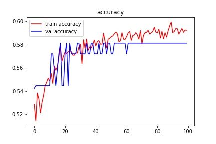
23:2   Encoder-Attention-Based Automatic Term Recognition (EA-ATR)

           Recently, deep learning methods are being widely used in many Natural Language
       Processing (NLP) related tasks and are improving the state-of-the-art of NLP [21] [6]. Such
       models attempt in an end-to-end manner to learn feature representations and perform
       classification.
           The most important factor in improving the current deep learning methods like Recurrent
       Neural Network (RNN) and Convolutional Neural Network (CNN) apart from efficiency and
       accuracy is the reduction in the dimension of inputs. We aim to generalize the task so that
       the model can be used on similar datasets. We attempt to achieve this by using a four-step
       strategy known as EEAP.
           Our main aim is to recognize the terms as precisely as possible, so it is important
       to understand the context between the sequence of words. Embeddings like GloVe and
       word2vec ignore this information. Therefore, we have used BERT (Bidirectional Encoder
       Representations from Transformers) to capture the contextual information [4] that helps
       recognize our proposed hypothesis better.
           The major contributions we like to mention here are; we have defined the traditional
       NLP task as a deep learning model which can be custom trained based on requirements.
       This model is effective in determining which sequence of words are terms compared to the
       statistical approach. We have also addressed the importance of contextual information in
       term recognition task in this tool by implementing BERT. Finally, in Section 5 we expose
       our results and show how our model outperformed the baseline model ATR4S referred in
       Section 2 by 28%. Our model also eliminates the need for multiple ranking and scoring
       algorithm to recognize terms in a given set of documents.

        2     Related Work
       Rule-based and statistical ATR researches
       Rule-based and statistical ATR methods [13] focused on parts-of-speech (PoS) for multi-word
       constituents. Such work contributed to the recognition of words by pattern-based approaches
       such as linguistic filters. Each word is tagged with its associated PoS in the linguistic filter
       system, and the domain-specific term is defined based on the tag. A list of terms identified by
       the linguistic filters (linguistic process) is commonly referred to as “candidate terms” (CT).
           Each sequence of words in the Candidate Terms (CT) (n-grams) is then given a score using
       statistical approaches. The score tells how likely the term is to be valid. The scores [13] are
       either the measures of “unithood”, which attempts to identify if multi-word CT constituents
       form a collocation rather than a co-occurrence by chance; or the measures of “termhood”
       focus on measuring how likely a candidate term, CT, is a domain-specific concept. The most
       commonly used technique to score the CT is to consider “frequency of occurrence”. The
       most recent term weighting scheme is TF-IDF which weights each term based on the number
       of occurrences within the document as well as within the entire corpora. These methods
       are used to filter the CT. Once filtered, because of their low ambiguity and high specificity,
       these extracted terms then can be used for many tasks including machine translation [5],
       information retrieval [15], ontology construction and ontology enrichment [2].

       Baseline Model: ATR4S
       Recent work on ATR is conducted by ART4S [1]. It comprises 13 state-of-the-art (SOTA)
       methods for ATR and implements the whole pipeline from text document pre-processing, to
       term candidate collection, term candidate scoring, and finally, term candidate ranking. The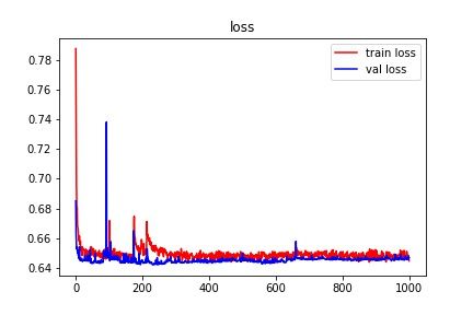
S. H. Manjunath and J. P. McCrae                                                                      23:3

text in the corpus is first split into sentences as part of pre-processing, tokenize and extract
part-of-speech tags and lemmas for obtained tokens. Once the texts are pre-processed, the
next step is “term candidate collection” – In this step, consecutive word n-grams (typically 1
to 4) of specified orders are extracted and three basic filters are applied (1. The noise filter:
To remove the unnecessary tags like HTML tags. 2. Stop word filter and 3. PoS tagging).
This gives a list of rare words. Words are then vectorized using the word2vec model. Each
word in the list is scored using 13 SOTA methods (TF-TDF, C-values, etc.,). Once the
scoring is done, the term is ranked to find how relevant a term is for being a key-term or
valid term.

Other related works

JATE 2.0 [24] is also closely related to ART4S [1] and uses 10 state-of-the-art methods and is
written in Java. Data is processed using traditional methods as in ART4S (pre-processing).
The pre-processed data is then passed to “candidate extraction”. JATE 2.0 uses Solr’s
analyzers for word vectorization which is a large text processing library. JATE 2.0 allows the
user to customize the analyzer based on individual needs. The obtained candidates are then
processed using different ATR algorithms which assigns the score and rank to the candidate
terms.
    AdaText [25] is another tool that is used in ATR. This tool improves on the TextRank
algorithm to generate better performance. This provides generic methods to improve
performance in any domain when coupled with an existing ATR method. AdaText uses
GloVe word embeddings on the 2 datasets. The main limitation of AdaText [25] is the
lack of understanding of the relation between the threshold used for selecting words on the
TextRank.
    All the works mentioned above provide some solution to identify domain-specific terms
but often result in an error-prone system due to the use of context-free models like word2vec
and GloVe. These models generate a single word embedding for each word in the CT,
resulting in unidirectional language models. This limits the choice of architecture that can
be used during pre-training [4]. Each candidate term needs to be evaluated not only based
on the frequency of occurrence but also the context. This contextual information is often
found on both the left-hand side and the right-hand side of the term. To address this issue a
new approach is proposed here – using BERT (Bidirectional Encoder Representations from
Transformers) embeddings.
    Stanford University has recently used BERT in its ATR method for glossary terms [10].
The focus is on biology terms for the online textbook, Inquire. They have used the CNN
along with BERT embedding to extract the terms for one domain (biology). The data was
prepared manually, and it is a laborious process. The embeddings are generated only for
unigram and hence the multi-word key-terms are ignored here.

   So far, all the rule-based methods and tools available for ATR used context-free models
and hence ignores the conceptual attribute for the term. Terms can be identified with
more accuracy if the contextual property is considered. There are recent advances in using
contextual models for term extraction [20] which uses BERT to fine-tune the terms extracted
using feature-based approach. In contrast, we propose the idea of using BERT embedding
which can capture the context of the given word and based on the context each candidate
term can be ranked. Our hypothesis here is that the term classified as key-term by this
process will be more accurate and reliable compared to other ATR tools.

                                                                                                    LDK 2021
23:4 Encoder-Attention-Based Automatic Term Recognition (EA-ATR)
3 Methodology
First, we use the Wikipedia titles as positive examples and generate random n-grams (of
length 1–4) as a possible set of negative terms. We filter out most of the unrelated n-grams
using Term Frequency - Inverse Document Frequency (TF-IDF), this ensures that we train
the model on challenging negative terms instead of random noise. If these n-grams are not
already present in our positive example, it is added as a weak negative example. Finally,
this dataset is transferred to a CSV for training purpose.
The model consists of BERT for embedding, Bi-LSTM for encoding, Attention for reducing
the input vector, ADAM optimizer [23] for training and a final prediction layer using a
sigmoid output forming the EEAP structure.
3.1 BERT embeddings
BERT can be used to extract features like word and sentence embedding vectors from text
data. These vectors are used as feature inputs to downstream NLP models like LSTM,
GRU, etc., NLP models require numerical vectors as inputs. Previously, texts were either
interpreted as uniquely indexed values (one-hot encoding) or more usefully as neural word
embedding where vocabulary words are mapped against fixed-length embedding features
resulting from models such as word2vec or Fasttext (does not consider the context within
which the word appears). BERT improves over word2vec by generating the embedding based
on the words around the text. This information is useful in ATR and hence, we have chosen
BERT embeddings.
The output representations from the BERT encoding layer are summed element-wise to
generate a single representation with shape (1, n, 768) for sequence embedding or (n,768) for
word embedding.
3.2 Encode
Provided a sequence of word vectors, the encode step generates a matrix where each row
represents the meaning of each token while paying attention to the context of the rest of the
sentence.
Figure 1 Encode [8].
In this project, we have used a bidirectional LSTM. LSTM is a variant of RNN which is
developed as a remedy to the problem of vanishing gradients and exploding gradients [7].
The key to solving the problem is by adding gates and a cell state to the RNN. A gate is a
non-linear function (usually a sigmoid) followed by multiplication.S. H. Manjunath and J. P. McCrae 23:5
3.3 Attend
The attend step reduces the size of the matrix produced by the encode step to a single vector.
In the process of reducing the matrix size, we lose most of the information. It is required to
retain important information and hence the context vector is crucial. This vector tells which
information to discard.
Figure 2 Attend [8].
We have employed an attention mechanism that learns the context vector as a parameter
in the model. This is inspired by the recent research conducted by Harbin Institute of
Technology [16] called “inner-attention”. Instead of using the target sentence to attend words
in the source sentence, inner-attention uses the sentence’s previous-stage representation to
attend to words that appeared. This approach results in a similar distribution of weights
compared to other attention mechanisms and assigns more weight to important words. This
approach produces precise and focused sentence representations for classification. Hence, the
“inner-attention” is selected for this step. It is inspired by the concept of how human can
roughly form a sense of which part of the sentence is important based on previous experiences.
Mathematically, this mechanism can be written as follows:
M = tanh(W y Y + W h Rave ⊗ eL ) (1)
α = sof tmax(wT M ) (2)
Ratt = Y αT (3)
where, Y is a matrix of output vectors of bi-LSTM, Rave is the output of mean pooling layer,
eL represents the bias matrix generated from the encoded input, α denotes the attention
vector and Ratt is the attention-weighted sentence representation. W y and W T M represents
the attentive weight matrix.
This process makes the attention mechanism a pure reduction task, which can replace the
sum or average pooling step.
LDK 202123:6 Encoder-Attention-Based Automatic Term Recognition (EA-ATR)
Figure 3 Predict [8].
3.4 Predict
Once the input data is reduced to a single vector, we can learn the target representation in
this step. Target representation may be a class label, a real value, a vector, etc. In our work,
the target representation is a class label. 0 if the sequence of words is non-terms and 1 if the
sequence of words contributes to being a term.
The predict layer is the last in our EEAP model. It receives the input from the attention
layer, a 2D tensor, and the input is passed through a dense layer with a “sigmoid” activation
function. Since we have to predict either 0 or 1, we have used the “sigmoid” function at the
last layer of the model i.e., the prediction layer. This function converts any real value into
another value in the range of 0 to 1. We map these predicted values to the probabilities
of the CT being a term. If the probability is less than 0.5 then it is not a term, or if the
probability is greater than 0.5 then it is classified as a term.
4 Experimental Settings
4.1 Data
There are two stages of data preparation for this model.
Stage 1 – Complete dataset preparation: Wikipedia titles are added to a list as positive
examples and random n-grams are added as weak negative examples, this list is called
candidate terms. If the generated n-gram is not in positive examples, then it is labelled
as 0 (a negative term). All the Wikipedia terms (positive term) are labelled ad 1. This
list of labelled data is converted into CSV to pass on to the next stage.
Stage 2 – Training and testing data preparation: The CSV file is loaded into the project.
The data is then divided into train and test data in an 80:20 ratio. The text and label
are separately loaded into the list from each train and test data. Text data is tokenized
using BERT’s FullTokenizer and padded to bring all input length to the same length.
This data is then passed to the BERT layer and then to the EEAP model to make the
prediction.
4.2 Model Architecture
The overall model architecture consists of several layers as explained below:
1. Embedding layer: This layer takes the BERT embedding matrix as input. The BERT
embedding is of shape (n, 768), where n is the vocabulary size. Once the embedding
matrix is passed through the embedding layer, the resulting output is a 3D tensor of
shape (batch_size, max_len, embedding_dim) i.e., (?,64, 768) in our case. The batch
size will be substituted at the run time.S. H. Manjunath and J. P. McCrae 23:7
2. Encode layer: A bidirectional LSTM layer is used as an encoding layer with 250 hidden
units, dropout and recurrent dropout is set to 0.1 which will drop the fraction of the
units for the linear transformation of the inputs and recurrent state respectively. The
resulting output is of shape (batch_size, max_len, hidden_units) i.e., (?, 64, 20).
3. Attention layer: The attention layer takes the input from the encoding layer (3D tensor)
and squeezes the input to 2D tensor and returns (batch_size, hidden_units) i.e., (?,
20). The main intention behind this step is input reduction by retaining only important
information. The reduction is done using the tanh activation function. A dot product
of the input matrix and weight along with the bias is passed to the activation function.
The result of the tanh lies in-between −1 and 1. The benefit is that negative inputs are
mapped highly negative and the zero inputs in the tanh graph are mapped near-zero thus
helping to retain only important information. Attention is also explained in Section 3.3
4. Feed Forward fully connected layer: A dense layer is a fully connected neural network
layer. We have specified 100 hidden units in the dense layer with the activation function
Rectified Linear Unit (ReLU). The number of units denotes the output size. Activation
in the dense layer sets the element-wise activation function to be used in the dense layer.
We have used multiple dense layers in the model with the last layer being activated with
the “sigmoid” activation function with 1 output node. Activation function selection is
explained in Section 4.3
5. Dropout layer: The dropout layer randomly sets the specified fraction of input nodes to
0 at each stage during training which helps prevent over-fitting. In this project, we are
using a single dropout layer with a 0.1 drop rate to avoid over-fitting. Figure 4 shows
how the model begins with over-fitting the data and over multiple iterations, the model
avoids over-fitting. This is achieved by the dropout layer. This value was selected as the
best fit after running the model with different fractions.
4.3 Hyper-parameters
Optimizer
Optimizers are algorithms or techniques used to adjust the neural network’s properties such
as weights and learning rate to reduce the losses. Optimizers help in getting the results faster.
We have used the Adam optimizer [12] [23] for building the EEAP structured model. Adam
optimizer is an extension of stochastic gradient descent with adaptive learning rate methods
to find individual learning rates for each parameter.
Loss Function
We have used the binary cross-entropy loss function as the problem we are trying to solve
here is, the binary classification problem.
Activation function
The sigmoid activation function (also called the logistic function), is a very popular activation
function for the neural network. The input to the function is transformed into a value
between 0.0 and 1.0. Since ours is a binary classification problem, we have used this function
in the last layer of the model to get the probability of the input being term, i.e., less than
0.5 is a non-term and greater than 0.5 is a term.
LDK 202123:8 Encoder-Attention-Based Automatic Term Recognition (EA-ATR)
Learning rate
The learning rate is a tuning parameter in an optimization algorithm that determines the size
of the step at each iteration while moving toward a minimum of a loss. Since it influences
the extent to which newly acquired information outweighs old information, it represents the
speed at which a machine learning model learns. We are setting the learning rate to 0.001
after running the model with different rates.
Decay/epsilon factor
Epsilon is the parameter used to avoid the divide by zero error when the gradient almost
reaches zero. Setting epsilon to a very small value would result in larger weight updates
and the optimizer becomes unstable. The bigger the value you set, the smaller the weights
updates and the model training process becomes slow. Therefore, we have chosen 0.0001 as
a good value for epsilon after running the model a few times with different values.
5 Results
Statistical Evaluation
The dataset used to train the model is Wikipedia titles as positive examples and random
n-grams as weak negative examples. The model is then evaluated against 2 other datasets –
GENIA [11] and Krapivin [14]. Table 1 gives the dataset description.
Table 1 Dataset description.
Dataset Domain Docs Words (thousands) Expected terms Source of terms
GENIA Bio medicine 2000 494 35,104 Authors’ keywords
Krapivin Computer science 2304 21 8766 Authors’ keywords
The candidate terms were extracted using the TF-IDF method and compared against the
expected terms from the datasets. Table 2 gives the candidate terms extracted across all the
datasets.
This way of filtering candidate terms is useful while we pass the entire document to the
model to predict the terms in it.
Table 2 Candidate terms.
Dataset N-grams Candidate terms Candidates among expected terms
GENIA 10000 7341 2659
krapivin 10000 7370 4150
EEAP model performance evaluation
The deep learning model is trained to recognize the terms with a total of 1,291,921 training
samples and 322,981 testing samples. The complete Wikipedia dataset consists of 1,614,902
samples with 1,314,902 positive examples and 300,000 negative examples.S. H. Manjunath and J. P. McCrae 23:9
We tested the model with different combination of hyper-parameters along with two
selected encoders LSTM and GRU to decide which of these combinations results in better
accuracy. The Food and Agriculture Organization (FAO) dataset is used for this evaluation.
The FAO dataset is described in Table 3.
Table 3 FAO dataset description.
Domain Agriculture
Docs 779
Words 26,672
Expected terms 1554
Source of terms Author’s keywords
Candidate terms 3895
Candidates among expected terms 862
We have used 0.001 as the learning rate since it is the standard learning rate set across the
optimizer. Encoders have 250 hidden nodes for all iterations. To avoid lengthy iteration and
due to resource constraints, we are considering the smaller dataset FAO for this comparison.
Table 4 gives the model evaluation result.
Table 4 Model performance for different hyper-parameter combinations on FAO dataset.
Encoder Optimizer F1-score Precision Recall Accuracy
GRU Adam 0.0673 0.6296 0.0355 56.3%
GRU SGD 0.0609 0.6183 0.0304 56.1%
GRU Adadelta 0.0609 0.6183 0.0304 56.1%
GRU RMSProp 0.073 0.653 0.0345 56.2%
LSTM Adam 0.1947 0.8253 0.1104 60.5%
LSTM SGD 0.0609 1.6183 0.0304 56.1%
LSTM Adadelta 0.6093 0.4381 1.0 43.8%
LSTM RMSProp 0.063 0.643 0.0335 55.2%
Along with the combination mentioned in Table 4, the loss function has also been changed
to other loss functions like “categorical cross-entropy”, “sparse categorical cross-entropy”.
Since this project is a binary classification, we are not moving further to use these loss
functions as it does not fit our problem definition. We have evaluated the model performance
with parameters that fit the project requirement and problem definition. After evaluating all
the experimental results, with LSTM as encoder, Adam optimizer and binary cross-entropy
loss function are selected as the best match for the model.
Figure 4 shows the model’s training and validation accuracy over 100 epochs. We can see
that the training accuracy keeps increasing over the iterations and this is because the model
learns in each iteration. In the beginning, the validation accuracy is more than training
accuracy which indicates over-fitting. Since we have used dropout layers in the model, the
model avoids over-fitting over the iterations. At around 50 iterations, training accuracy
crosses over validation accuracy. This indicates that the model is now learning for the
training data efficiently.
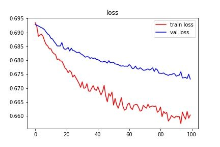
Figure 5 shows the loss incurred over 100 epochs. The loss function intends to make
the model learn. The loss is propagated back to the hidden nodes and the model learns to
minimize these losses. Our model’s loss keeps decreasing over the iterations and this shows
that the model is learning better in each step. We further ran the model for 1000 iteration
to find the convergence, Figure 6 shows the convergence.
LDK 202123:10 Encoder-Attention-Based Automatic Term Recognition (EA-ATR)
Figure 4 Model accuracy over 100 iteration.
Figure 5 Decrease in loss over 100 iteration.
Evaluation on different dataset
The model is evaluated against two different datasets – GENIA and Krapivin as mentioned
in Section 5. Table 5 shows the evaluation of these two datasets. The result is also evaluated
against the base model ATR4S [1] and results are included in the Table 5. The FAO dataset
used here is the held-out data to perform the evaluation.
Table 5 Evaluation on different datasets.
Comparison – EA-ATR(A) vs ATR4S(B) EA-ATR model
Dataset A precision B precision A accuracy B accuracy F1-score Recall
GENIA 0.8045 0.7760 60% 24% 0.7460 0.6955
Krapivin 0.6345 0.4279 62% 42% 0.7612 0.9511
(ATR4S model recall and F1-score not available for comparison)S. H. Manjunath and J. P. McCrae 23:11
Figure 6 Convergence in loss over 1000 iteration.
Along with the precision, recall and accuracy metrics, we can extract the confusion matrix
to evaluate the performance of the classifier. The idea is to count the number of times terms
are classified as non-terms and vice-versa. Figure 7 shows the confusion matrix on evaluation
dataset (FAO Terms).
Figure 7 Confusion Matrix.
The model is well trained in predicting the non-terms. It is important to differentiate
non-terms from terms because the ratio of non-terms in the document is more compared to
terms. Although the model is a little biased towards non-terms, which is mainly because of
the domain-specific dataset we are using, the model performs better considering the dataset
used to train the model. This model stands as a new state-of-the-art for ATR using deep
learning techniques. The model performs overall 28% better than the base model [1].
LDK 202123:12 Encoder-Attention-Based Automatic Term Recognition (EA-ATR)
6 Conclusion
Current advances in NLP frameworks and applications focused on deep learning [22] have
achieved better efficiency over many state-of-the-art NLP tasks, such as question answering
and machine translation. This research is an attempt to show that deep learning models
perform better and are more reliable than conventional automatic term recognition algorithms.
The model performs 28% better than the ATR4S [1] base model. The model also performs
remarkably well on the GENIA and Kraplivin evaluation datasets. The simulations are a
clear example of a deep learning model being applied to NLP tasks by reducing the repetitive
computational requirement for each dataset and extracting automatic terms more precisely.
This method has the potential to be used as a multilingual model as it does not require
any annotations. This is a future enhancement we would like to experiment with and see
how well this works for different analytic and synthetic languages.
References
1 Nikita Astrakhantsev. ATR4S: toolkit with state-of-the-art automatic terms recognition
methods in Scala. Language Resources and Evaluation, 52(3):853–872, 2018.
2 Nikita A Astrakhantsev, Denis G Fedorenko, and D Yu Turdakov. Methods for automatic
term recognition in domain-specific text collections: A survey. Programming and Computer
Software, 41(6):336–349, 2015.
3 James R Curran and Marc Moens. Improvements in automatic thesaurus extraction. In
Proceedings of the ACL-02 workshop on Unsupervised lexical acquisition, pages 59–66, 2002.
4 Jacob Devlin, Ming-Wei Chang, Kenton Lee, and Kristina Toutanova. BERT: pre-training
of deep bidirectional transformers for language understanding. arXiv preprint, 2018. arXiv:
1810.04805.
5 Éric Gaussier. Flow network models for word alignment and terminology extraction from
bilingual corpora. In Proceedings of the 36th Annual Meeting of the Association for Computa-
tional Linguistics and 17th International Conference on Computational Linguistics - Volume 1,
ACL ’98/COLING ’98, page 444–450, USA, 1998. Association for Computational Linguistics.
doi:10.3115/980845.980921.
6 Kaiming He, Xiangyu Zhang, Shaoqing Ren, and Jian Sun. Deep residual learning for image
recognition. In Proceedings of the IEEE conference on computer vision and pattern recognition,
pages 770–778, 2016.
7 Sepp Hochreiter and Jürgen Schmidhuber. Long short-term memory. Neural computation,
9(8):1735–1780, 1997.
8 Matthew Honnibal. Embed, encode, attend, predict: The new deep learning formula for
state-of-the-art NLP models. Blog, Explosion, November, 10, 2016.
9 Kyo Kageura and Bin Umino. Methods of automatic term recognition: A review. Terminology.
International Journal of Theoretical and Applied Issues in Specialized Communication, 3(2):259–
289, 1996.
10 Kush Khosla, Robbie Jones, and Nicholas Bowman. Featureless deep learning methods for
automated key-term extraction, 2019. URL: https://web.stanford.edu/class/archive/cs/
cs224n/cs224n.1194/reports/custom/15848334.pdf.
11 J-D Kim, Tomoko Ohta, Yuka Tateisi, and Jun’ichi Tsujii. GENIA corpus—a semantically
annotated corpus for bio-textmining. Bioinformatics, 19(suppl_1):i180–i182, 2003.
12 Diederik P Kingma and Jimmy Ba. Adam: A method for stochastic optimization. arXiv
preprint, 2014. arXiv:1412.6980.
13 Ioannis Korkontzelos, Ioannis P. Klapaftis, and Suresh Manandhar. Reviewing and evaluating
automatic term recognition techniques. In Bengt Nordström and Aarne Ranta, editors,
Advances in Natural Language Processing, pages 248–259, Berlin, Heidelberg, 2008. Springer
Berlin Heidelberg.S. H. Manjunath and J. P. McCrae 23:13
14 Mikalai Krapivin, Aliaksandr Autaeu, and Maurizio Marchese. Large dataset for keyphrases
extraction. Technical report, University of Trento, 2009.
15 Yang Lingpeng, Ji Donghong, Zhou Guodong, and Nie Yu. Improving retrieval effectiveness by
using key terms in top retrieved documents. In David E. Losada and Juan M. Fernández-Luna,
editors, Advances in Information Retrieval, pages 169–184, Berlin, Heidelberg, 2005. Springer
Berlin Heidelberg.
16 Yang Liu, Chengjie Sun, Lei Lin, and Xiaolong Wang. Learning natural language inference
using bidirectional LSTM model and inner-attention. arXiv preprint, 2016. arXiv:1605.09090.
17 Diana Maynard, Yaoyong Li, and Wim Peters. NLP techniques for term extraction and
ontology population, 2008.
18 Shervin Minaee, Nal Kalchbrenner, Erik Cambria, Narjes Nikzad, Meysam Chenaghlu, and
Jianfeng Gao. Deep learning based text classification: A comprehensive review. arXiv preprint,
2020. arXiv:2004.03705.
19 Michael P Oakes and Chris D Paice. Term extraction for automatic abstracting. D. Bourigault,
C. Jacquemin, and MC. L’Homme, editors, Recent Advances in Computational Terminology,
2:353–370, 2001.
20 Ayla Rigouts Terryn, Veronique Hoste, Patrick Drouin, and Els Lefever. TermEval 2020:
Shared task on automatic term extraction using the annotated corpora for term extraction
research (ACTER) dataset. In Proceedings of the 6th International Workshop on Computa-
tional Terminology, pages 85–94, Marseille, France, May 2020. European Language Resources
Association. URL: https://www.aclweb.org/anthology/2020.computerm-1.12.
21 Ashish Vaswani, Noam Shazeer, Niki Parmar, Jakob Uszkoreit, Llion Jones, Aidan N Gomez,
Łukasz Kaiser, and Illia Polosukhin. Attention is all you need. In Advances in neural
information processing systems, pages 5998–6008, 2017.
22 Tom Young, Devamanyu Hazarika, Soujanya Poria, and Erik Cambria. Recent trends in deep
learning based natural language processing. CoRR, abs/1708.02709, 2017. arXiv:1708.02709.
23 Zijun Zhang. Improved Adam optimizer for deep neural networks. In 2018 IEEE/ACM 26th
International Symposium on Quality of Service (IWQoS), pages 1–2. IEEE, 2018.
24 Ziqi Zhang, Jie Gao, and Fabio Ciravegna. JATE 2.0: Java automatic term extraction with
apache Solr. In Proceedings of the Tenth International Conference on Language Resources
and Evaluation (LREC’16), pages 2262–2269, Portorož, Slovenia, 2016. European Language
Resources Association (ELRA). URL: https://www.aclweb.org/anthology/L16-1359.
25 Ziqi Zhang, Johann Petrak, and Diana Maynard. Adapted textrank for term extraction:
A generic method of improving automatic term extraction algorithms. Procedia Computer
Science, 137:102–108, January 2018. doi:10.1016/j.procs.2018.09.010.
LDK 2021You can also read