Evaluating the Potential of GloFAS-ERA5 River Discharge Reanalysis Data for Calibrating the SWAT Model in the Grande San Miguel River Basin El ...
←
→
Page content transcription
If your browser does not render page correctly, please read the page content below
remote sensing
Article
Evaluating the Potential of GloFAS-ERA5 River Discharge
Reanalysis Data for Calibrating the SWAT Model in the Grande
San Miguel River Basin (El Salvador)
Javier Senent-Aparicio 1, * , Pablo Blanco-Gómez 1 , Adrián López-Ballesteros 1 , Patricia Jimeno-Sáez 1
and Julio Pérez-Sánchez 1,2

                                           1   Department of Civil Engineering, Universidad Católica San Antonio de Murcia, Campus de Los Jerónimos
                                               s/n, 30107 Murcia, Spain; pblanco4@alu.ucam.edu (P.B.-G.); alopez6@ucam.edu (A.L.-B.);
                                               pjimeno@ucam.edu (P.J.-S.); jperez058@ucam.edu (J.P.-S.)
                                           2   Department of Civil Engineering, Universidad de Las Palmas de Gran Canaria, Campus de Tafira,
                                               35017 Las Palmas de Gran Canaria, Spain
                                           *   Correspondence: jsenent@ucam.edu; Tel.: +34-968-278-769

                                           Abstract: Hydrological modelling requires accurate climate data with high spatial-temporal resolu-
                                           tion, which is often unavailable in certain parts of the world—such as Central America. Numerous

                                    studies have previously demonstrated that in hydrological modelling, global weather reanalysis
Citation: Senent-Aparicio, J.;             data provides a viable alternative to observed data. However, calibrating and validating models
Blanco-Gómez, P.; López-Ballesteros, A.;   requires the use of observed discharge data, which is also frequently unavailable. Recent, global-scale
Jimeno-Sáez, P.; Pérez-Sánchez, J.         applications have been developed based on weather data from reanalysis; these applications allow
Evaluating the Potential of                streamflows with satisfactory resolution to be obtained. An example is the Global Flood Awareness
GloFAS-ERA5 River Discharge                System (GloFAS), which uses the fifth generation of reanalysis data produced by the European Centre
Reanalysis Data for Calibrating the        for Medium-Range Weather Forecasts (ERA5) as input. It provides discharge data from 1979 to the
SWAT Model in the Grande San               present with a resolution of 0.1◦ . This study assesses the potential of GloFAS for calibrating hydro-
Miguel River Basin (El Salvador).
                                           logical models in ungauged basins. For this purpose, the quality of data from ERA5 and from the
Remote Sens. 2021, 13, 3299. https://
                                           Climate Hazards Group InfraRed Precipitation and Temperature with Station as well as the Climate
doi.org/10.3390/rs13163299
                                           Forecast System Reanalysis (CFSR) was analysed. The focus was on flow simulation using the Soil
                                           and Water Assessment Tool (SWAT) model. The models were calibrated using GloFAS discharge data.
Academic Editors: Sandra G.
García Galiano, Fulgencio
                                           Our results indicate that all the reanalysis datasets displayed an acceptable fit with the observed
Cánovas García and Juan                    precipitation and temperature data. The correlation coefficient (CC) between the reanalysis data and
Diego Giraldo-Osorio                       the observed data indicates a strong relationship at the monthly level all of the analysed stations
                                           (CC > 0.80). The Kling–Gupta Efficiency (KGE) also showed the acceptable performance of the
Received: 12 July 2021                     calibrated SWAT models (KGE > 0.74). We concluded that GloFAS data has substantial potential for
Accepted: 18 August 2021                   calibrating hydrological models that estimate the monthly streamflow in ungauged watersheds. This
Published: 20 August 2021                  approach can aid water resource management.

Publisher’s Note: MDPI stays neutral       Keywords: SWAT; satellite weather dataset; ERA-5; GloFAS; hydrological modelling; El Salvador
with regard to jurisdictional claims in
published maps and institutional affil-
iations.

                                           1. Introduction
                                                Hydrological models are commonly used to understand changes in hydrological
                                           processes due to changes in the climatic or the land use [1,2]. Such changes in land use
Copyright: © 2021 by the authors.
                                           and climatic conditions are especially important in Central America. Recent studies have
Licensee MDPI, Basel, Switzerland.
                                           highlighted deforestation as the main land-use change in this area [3]. However, climate
This article is an open access article
                                           change can also strongly affect the hydrological cycle by altering the timing and intensity
distributed under the terms and
                                           of rainfall, recharge and runoff. This change has intensified the mid-summer drought
conditions of the Creative Commons
                                           characteristic of Central America’s weather [4].
Attribution (CC BY) license (https://
creativecommons.org/licenses/by/
                                                In addition to forecasting and estimating the quantity and quality of water for decision-
4.0/).
                                           makers, hydrological models can assist local authorities in forecasting the effects of natural

Remote Sens. 2021, 13, 3299. https://doi.org/10.3390/rs13163299                                      https://www.mdpi.com/journal/remotesensing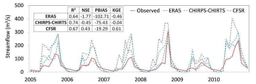
Remote Sens. 2021, 13, 3299                                                                                           2 of 20

                              and anthropogenic changes on water resources. Furthermore, they can characterise the
                              temporal and spatial availability of water resources to enable the design of appropriate
                              strategies to mitigate water-related hazards. These includes droughts, floods and the
                              discharge of pollutants.
                                    Several conceptual and semi-distributed models have been applied at grid scale in
                              tropical climatology. Srivastava et al. (2017) [5] successfully implemented the variable
                              infiltration capacity (VIC) model for the Kangsabati River Basin and obtained satisfactory
                              evapotranspiration estimates at the monthly scale. Srivastava et al. (2020) [6] compared
                              two models, namely VIC and the model for the identification of unit hydrograph and
                              components flows from rainfall, evapotranspiration and streamflow (IHACRES). They
                              concluded that IHACRES is a very useful model for data-scarce regions. Paul et al. (2018) [7]
                              similarly reported the successful implementation of a modified time-variant spatially
                              distributed hydrograph technique integrated into the satellite-based hydrological model
                              (SHM) for the Kabini River Basin.
                                    The distributed Soil and Water Assessment Tool (SWAT) model has also been widely
                              used in tropical basins [8]. Darbandsari and Coulibaly (2020) [9] demonstrated the useful-
                              ness of lumped hydrological models for simulating hydrological processes in data-scarce
                              watersheds. However, in the current study, the distributed SWAT model is used, because
                              once calibrated, it allows further analyses related to land-use changes. SWAT is one of
                              several models employed to assess the influence of land use and land management changes
                              on water resources [10].
                                    Accuracy in simulating a basin’s water resources fundamentally depends on the input
                              data used for modelling and on the capability of the hydrological model. Primary input
                              data are meteorological and geographical data (e.g., precipitation and temperature as well
                              as data from digital elevation models and land-use and soil maps). In recent years, several
                              ready-to-use global-scale maps have been developed that provide good results and make
                              the SWAT model application easier [11].
                                    The application of hydrological models is usually limited by the sparse distribution of
                              rainfall observation stations. In most watersheds, the actual density of a rainfall network is
                              notably lower than the values recommended by the World Meteorological Organization.
                              Ground-based precipitation observation is also unevenly distributed in many countries
                              due to economic constraints [12], and this issue can affect model estimates of streamflow
                              performance. Missing values in rainfall data negatively affect the quality of hydrological
                              modelling. Tan and Yang (2020) [13] demonstrated that missing values of more than
                              20% significantly affected the streamflow simulation for tropical climates. To overcome
                              limitations arising from the scarcity of data or from poor-quality observations, numerous
                              studies have compared gridded rainfall datasets with local datasets. The aim is to assess
                              their suitability of those datasets in various hydrological models [14–17] for watersheds
                              around the world.
                                    The influence of temperature data on hydrological balance and discharge in simulated
                              river basins has rarely been analysed (Tan et al., 2021).               In Southeast Asia,
                              Tan et al. (2017) [18] recommended combining the Asian Precipitation Highly Resolved
                              Observational Data Integration Towards Evaluation (APHRODITE) dataset [19] with the
                              maximum and minimum temperatures from the Climate Forecast System Reanalysis
                              (CFSR) dataset [20]. The objective was to model ungauged or gauge-limited catchments. In
                              Ethiopia, Duan et al. (2019) [21] recommended the use of Climate Hazards Group Infrared
                              Precipitation with Stations (CHIRPS) data [22] together with temperature data from CFSR
                              for hydrological modelling.
                                    Due to advances in satellite technology, many satellite weather products have been
                              developed to monitor weather conditions on a global scale. Some are called reanalysis
                              products; they combine satellite data with observed data to improve weather representation.
                              An example is the CFSR dataset. It is widely used for hydrological modelling in the
                              SWAT model, because—in addition to precipitation—it includes other meteorological
                              variables that are easily downloadable from the SWAT website [23]. Additional reanalysis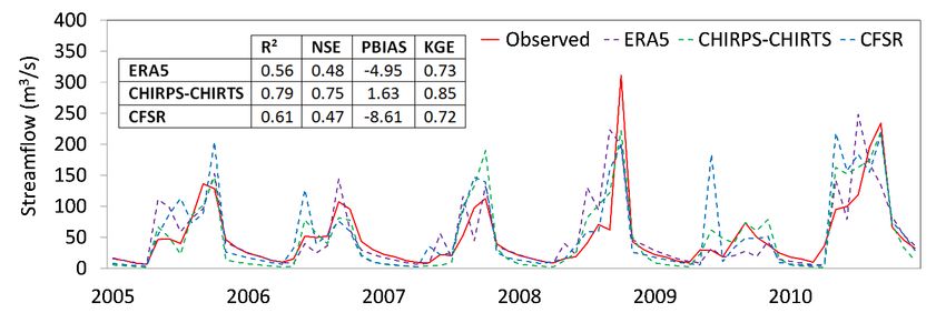
Remote Sens. 2021, 13, 3299                                                                                          3 of 20

                              datasets that include precipitation and temperature data for simulations have recently been
                              launched. For example, the CHIRPS precipitation dataset has recently been complemented
                              with temperature data to yield the Climate Hazards Center InfraRed Temperature with
                              Stations CHIRTS [24]. This data is available for the global scale at a spatial resolution
                              of 0.05◦ .
                                    Another recently launched dataset that includes precipitation and temperature is
                              the ERA5 global reanalysis dataset [25]. It provides data from 1950 to the present at
                              a spatial resolution of 31 km. It was released recently and has not yet been tested in
                              hydrological modelling for several areas of the world. However, Tarek et al. (2020) [26]
                              tested the potential of ERA5 in hydrological modelling across North America. Their results
                              highlighted many advantages over the previous dataset, ERA-Interim, and demonstrated
                              a level of efficiency similar to that obtained in hydrological models that use observed
                              data for most of the territory analysed. Kolluru et al. (2020) [27] concluded that ERA5 is
                              efficient for detecting rainfall patterns, whereas CHIRPS dysplays better flow simulation.
                              Jiang et al. (2021) [28] obtained highly varying results depending on the regions analysed
                              and identified the general underestimation of extreme rainfall.
                                    Model calibration and validation are key steps for obtaining accurate estimates of
                              streamflow from hydrological models. These steps are generally performed using observed
                              data [29]. However, in situ flow data are commonly unavailable for much of the land area,
                              especially in developing countries, and the number of operational stations is decreasing
                              rapidly. The recent availability of global-scale remote sensing climate products (such as
                              those discussed above) has led to the development of hydrological models that provide
                              discharge estimates at a global scale [30–32].
                                    One such application is the Global Flood Awareness System (GloFAS), developed
                              by the European Centre for Medium-Range Weather Forecasts (ECMWF) in collaboration
                              with the University of Reading and the Joint Research Centre of the European Commission.
                              This system couples the Hydrology Tiled ECMWF Scheme for Surface Exchanges over
                              Land (HTESSEL) [33] and LISFLOOD models [34]; it provides streamflow estimates at
                              a global scale from 1979 to the present, using ERA5 as the climatological input data.
                              Global hydrological models are powerful tools for reconstructing components of the water
                              balance because they generate continuous data, which can be used in applications such as
                              hydrological model calibration [35]. Given the recent release of GloFAS, its potential has
                              not been fully explored.
                                    Central America is an area in which remotely sensed data can be highly useful for
                              hydrological modelling to improve estimates of water resources [36]. Tan et al. (2021) [37]
                              reviewed 123 articles regarding the use of alternative climate products in SWAT modelling.
                              The authors found only one study conducted in Mexico and no precedents of this type of
                              study for Central America.
                                    In light of the above, this work may be of interest to stakeholders who model water-
                              sheds located in Central America. We selected the Grande San Miguel (GSM) River Basin
                              as a case study, because many of the problems discussed above occur there. These include
                              a low density of stations that provide precipitation and temperature records, a substantial
                              percentage of missing data, and difficulty in obtaining streamflow data to enable model
                              calibration. Using monthly flow data provided by the Ministry of Environment and Nat-
                              ural Resources in El Salvador for the period 2005–2010, we explored the potential of the
                              GLoFAS-ERA5 river discharge reanalysis dataset for calibrating hydrological models in
                              ungauged watersheds. The use of remotely sensed rainfall data for hydrological simulation
                              is common in recent literature [37]. However, the use of globally generated flow data from
                              remotely sensed data for calibrating a hydrological models is very novel because the release
                              of these products is so recent [38,39].
                                    This paper addresses the following objectives: (1) to evaluate the performance of pre-
                              cipitation and temperature variables using satellite reanalysis data such as CFSR, CHIRPS
                              and ERA5 throughout the GSM River Basin; and (2) to assess the GLoFAS-ERA5 river
                              discharge reanalysis dataset’s potential for calibrating hydrological models and its relation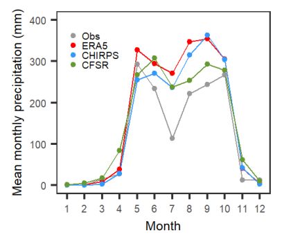
Remote Sens. 2021, 13, 3299 4 of 20
to precipitation and temperature reanalysis data used as input data. To date, few stud-
ies [21,40] have analysed the effectiveness of reanalysis data that includes temperature
for simulating hydrological processes in a watershed. Most studies have considered only
precipitation data.
2. Study Area and Weather Data Sources
2.1. Study Area
The GSM River Basin is geographically located in the east of El Salvador; it covers
2377 km2 up to the outlet control point (Figure 1). The basin is among the largest in El
Salvador. The city of San Miguel is situated at its core and is El Salvador’s second most
populous city. The basin is ecologically sensitive in terms of international protection, such
as the protected zones of Tepaca-San Miguel and Jiquilisco Bay. Tecapa-San Miguel is
known for its coffee plantations, coastal plain wetlands, and volcanic craters; the area
includes several lagoons listed under the Ramsar Convention on Wetlands. Since 2005, the
Remote Sens. 2021, 13, 3299 5 of 19
Jiquilisco Bay—which is located at the mouth of the Grande de San Miguel River—has
been designated as a Ramsar site and a UNESCO biosphere reserve.
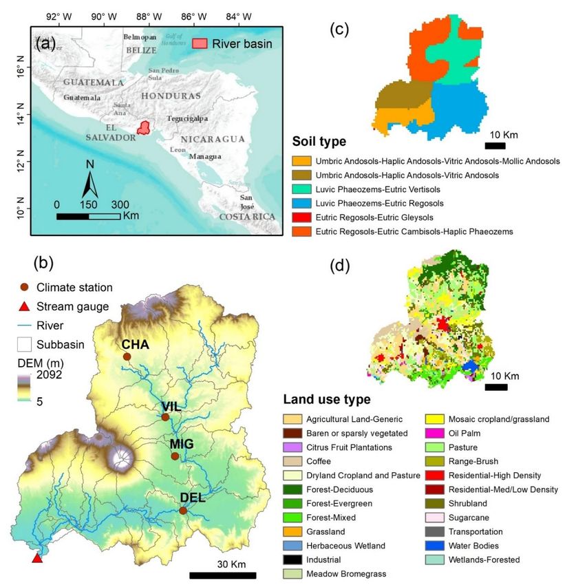
Figure 1. The study area location: (a) location of the Grande San Miguel river basin in Central America, (b) digital elevation
Figure 1. The study area location: (a) location of the Grande San Miguel river basin in Central
model (DEM), sub-basins, and river stream delineation in the Grande San Miguel river basin, (c) soil map, and (d) land-
America,
use map. (b) digital elevation model (DEM), sub-basins, and river stream delineation in the Grande
San Miguel river basin, (c) soil map, and (d) land-use map.
2.2. In Situ Rainfall and Temperature Data
Figure 1 shows the spatial distribution of rainfall stations in the GSM River Basin.
Most of the existing weather stations are located in the lowlands, between 100 m and 200
m above sea level. As indicated in Table 1, three of the four available meteorological sta-
tions had more than 20% of data missing during the period under study (2005–2010). Ac-
cording to Tan and Yang (2020) [13], missing data of more than 20% significantly affects
the simulation of flows in tropical climates. Given this fact and the low density of available
stations, we used observed data to analyse the performance of the rainfall and tempera-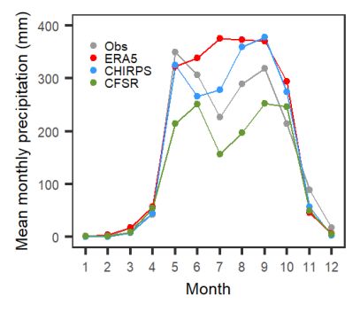
Remote Sens. 2021, 13, 3299                                                                                                               5 of 20

                                          Polluted water and the potential need for agricultural water are the two most pressing
                                    challenges in the GSM River Basin. [41]. To propose effective governance methods to
                                    mitigate the effect of these stress factors, the precise simulation of hydrological processes at
                                    the basin scale is crucial.
                                          This region’s climate is tropical, with high annual precipitation rates. However, the
                                    intra-annual distribution is uneven, with 90% of precipitation falling during the rainy
                                    season between May and October and scattered showers occurring during the dry season
                                    between November and April [36,42]. According to weather station measurements, the
                                    average annual precipitation is 1700 mm. The wettest months are from May to October
                                    and the driest months are from November to April. The basin is occasionally crossed
                                    by hurricanes, especially in September and October, which cause substantial flooding.
                                    Maximum temperatures are as high as 37 ◦ C, and minimum temperatures drop to 17 ◦ C.
                                    The altitude ranges from sea level to higher than 2000 m at the San Miguel Volcano.
                                          Andosols, phaeozems, and regosols are the three most common soil types in the area
                                    (Figure 1c). The andosols that cover the area around the San Miguel Volcano are volcanic
                                    soils, which are highly permeable and have ideal agricultural qualities [43]. Regosols are
                                    unconsolidated materials with fine granulometry, common in mountainous areas. This
                                    is the dominant soil type at the northern boundaries. By contrast, phaeozem soils are
                                    abundant in the eastern part of the basin; they accommodate wet grasslands and forest
                                    regions because they are porous and fertile, and they provide excellent agricultural land
                                    (FAO, 2008). Grassland and pasture (43%), crops (32%), and forest (17%) are the most
                                    common land uses. The land-use map of the basin is shown in Figure 1d.

                                    2.2. In Situ Rainfall and Temperature Data
                                          Figure 1 shows the spatial distribution of rainfall stations in the GSM River Basin.
                                    Most of the existing weather stations are located in the lowlands, between 100 m and
                                    200 m above sea level. As indicated in Table 1, three of the four available meteorological
                                    stations had more than 20% of data missing during the period under study (2005–2010).
                                    According to Tan and Yang (2020) [13], missing data of more than 20% significantly affects
                                    the simulation of flows in tropical climates. Given this fact and the low density of available
                                    stations, we used observed data to analyse the performance of the rainfall and temperature
                                    reanalysis data, but we did not simulate flows based on observed data.

                                       Table 1. Summary of the weather stations used in this study.

                                                                                                                            Missing Data
          Code                  Station              Latitude (◦ )          Longitude (◦ )          Elevation (m)
                                                                                                                               (%) 1
          MIG                 San Miguel                13.4690               −88.1590                    98                   11.3/1.2
          CHA                 Chapeltique               13.6424               −88.2608                    207                    25.4
          DEL                  El Delirio               13.3274               −88.1416                    92                     41.4
          VIL                  Villerías                13.5187               −88.1795                    109                    51.7
      1 At San Miguel station, daily precipitation and temperature data are obtained. The percentages of missing data on precipitation and
      temperature data are 11.3% and 1.2% respectively.

                                    2.3. Reanalysis Precipitation and Temperature Datasets Used in This Study
                                    2.3.1. ERA5 Reanalysis Dataset
                                         The ECMWF’s most advanced reanalysis output is ERA5. This output was recently
                                    released with a resolution of roughly 30 km and can be used to compute many atmospheric
                                    variables from January 1950 to near real-time [25]. In the current study, the ERA5 hourly
                                    rainfall and temperature were extracted from the toolbox available on the Copernicus
                                    Climate Data Store website (https://cds.climate.copernicus.eu, accessed on 1 April 2021)
                                    and aggregated to the daily time step.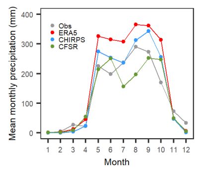
Remote Sens. 2021, 13, 3299                                                                                            6 of 20

                              2.3.2. CHIRPS and CHIRTS
                                   The CHIRPS dataset is the result of a collaboration between the United States Geologi-
                              cal Survey and the University of California. It consists of a rainfall grid with a geographical
                              resolution of 0.05◦ that combines data from satellites with data from on-site rainfall stations.
                              The dataset was created using the following sources [22]:
                              •    the Tropical Rainfall Measuring Mission (TRMM) 3B42 product from NASA
                              •    the monthly precipitation climatology (CHPClim)
                              •    atmospheric model rainfall fields from the National Oceanic and Atmospheric Admin-
                                   istration (NOAA) Climate Forecast System version 2 (CFSv2)
                              •    quasi-global geostationary thermal infrared (IR) satellite observations from two
                                   NOAA sources
                              •    in situ rainfall observations
                                   More recently, a temperature dataset with the same spatial resolution as CHIRPS has
                              been developed on a daily scale. It entailed merging the monthly CHIRTS and disaggregat-
                              ing the monthly data using daily temperatures from ERA5 [24]. On the Climate Hazards
                              Group website (https://www.chc.ucsb.edu/data/, accessed on 5 April 2021), users can
                              obtain daily CHIRPS v2.0 and CHIRTS v1.0 data.

                              2.3.3. CFSR
                                   The CFSR product was developed by the National Centers for Environmental Pre-
                              diction (NCEP) [44]. It uses advanced data-assimilation methods and data from a global
                              network of weather stations and satellite-based products; it also draws on complex atmo-
                              spheric, oceanic, and surface modelling elements coupled with a resolution of 0.30◦ and
                              covering any land location in the world [20]. The available CFSR data is available for 1979
                              to 2014 and can be downloaded from the SWAT website (https://globalweather.tamu.edu/,
                              accessed on 5 April 2021).

                              2.4. GloFAS River Discharge Reanalysis Dataset
                                   The GloFAS is part of the Copernicus Emergency Management Service (CEMS). The
                              dataset was developed through collaboration between the ECMWF, the Joint Research
                              Centre of the European Commission and the University of Reading (www.globalfloods.eu,
                              accessed on 22 March 2021). The GLoFAS river discharge reanalysis dataset is a product of
                              CEMS and is produced by coupling surface and subsurface runoff data from the HTESSEL
                              surface model used forced by ERA5 reanalysis data [25] with the Distributed Water Balance
                              and Flood Simulation (LISFLOOD) hydrological and channel routing model [34].
                                   The model was calibrated using more than a thousand flow stations located in
                              66 different countries. It achieved a median Kling–Gupta efficiency (KGE) values of 0.67
                              and a correlation value of 0.80 [35]. The river discharge reanalysis, with daily time steps
                              and 0.1◦ spatial resolution, is freely available to download for the period 1979 until near-
                              present through the Copernicus Climate Data Store (https://cds.climate.copernicus.eu,
                              accessed on 1 April 2021).

                              3. Materials and Methods
                                    The methodological approach followed in this study is illustrated in Figure 2. It con-
                              sisted of two main steps: (1) a comparison of rainfall and temperature data from reanalysis
                              products with observed weather gauge data; and (2) an evaluation of the applicability of
                              the flow data available in GLoFAS for the calibration of the SWAT hydrological model on a
                              monthly scale. In the latter step, the weather input data used were ERA5, CHIRPS-CHIRTS
                              and CFSR.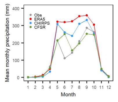
The methodological approach followed in this study is illustrated in Figure 2. It co
                                               sisted of two main steps: (1) a comparison of rainfall and temperature data from reanaly
                                               products with observed weather gauge data; and (2) an evaluation of the applicability
                                               the flow data available in GLoFAS for the calibration of the SWAT hydrological model
Remote Sens. 2021, 13, 3299                    a monthly scale. In the latter step, the weather input data used were 7ERA5,
                                                                                                                          of 20 CHIRP
                                               CHIRTS and CFSR.

                              Figure 2. Flowchart of the methodological approach used in this study.
                                              Figure 2. Flowchart of the methodological approach used in this study.
                                   To perform the evaluation, streamflows were first assessed using each of the reanal-
                                                  To perform the evaluation, streamflows were first assessed using each of the rean
                              ysis products as input values; the monthly streamflows were simulated from the default
                                             ysis products as input values; the monthly streamflows were simulated from the defa
                              values of the parameters in the SWAT model. Second, each simulation was calibrated
                                             values of the parameters in the SWAT model. Second, each simulation was calibrated
                              independently using the GLoFAS data as the observed data. Finally, the accuracy of the
                                             dependently using the GLoFAS data as the observed data. Finally, the accuracy of t
                              GLoFAS-calibrated models for reproducing the observed monthly flows was assessed.
                                             GLoFAS-calibrated models for reproducing the observed monthly flows was assessed.
                              3.1. SWAT Model Description
                                    The SWAT model is a physically based and distributed, and continuous, time model.
                              It is used to model rainfall runoff at the basin scale [10]. Several global studies have
                              applied the SWAT model to investigate hydrological and water quality processes [45–47],
                              the impact of human pressure on water resources [48–50], and the consequences of cli-
                              mate change [36,51–53]. The model’s GIS interface [54] allows for simple and quick data
                              processing, such as watershed delineation and spatial and tabular data handling.
                                    A watershed is divided into multiple sub-watersheds by SWAT. These are further
                              subdivided into hydrological response units (HRUs), which include homogeneous land
                              use, soil, and land slope. Water balance components, sediment flow, plant development
                              and nutrient loss are some of the major processes that the model can replicate. To simulate
                              the water balance components, SWAT solves the following equation:

                                                              t
                                                  SWt = SW0 + ∑ Rday − Qsur f − Ea − Wseep − Q gw ,                         (1)
                                                                  i =1

                              where SWt is the final soil water content (mm), SW0 is the initial soil water content (mm),
                              t is the time in days, Rday is the precipitation (mm), Qsur f is the surface runoff (mm), Ea
                              is the evapotranspiration (mm), Wseep is the percolation (mm) and Q gw is the return flow
                              (mm). Neitsch et al. (2012) [55] provide more information on the operation of the SWAT
                              hydrological model.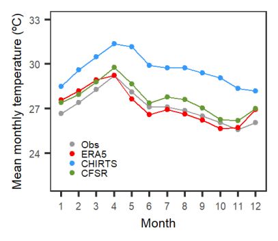
Remote Sens. 2021, 13, 3299                                                                                                      8 of 20

                                     3.2. SWAT Model Setup
                                          We used the QGIS interface for SWAT, namely QSWAT version 3 [54], to build the
                                     model with publicly available information. In this study, the spatial data for the SWAT
                                     model includes a digital terrain model, land-use map, and soil map. For basin delineation,
                                     we acquired the Advanced Spaceborne Thermal Emission and Reflection Radiometer
                                     Global Digital Elevation Model (ASTER GDEM) from the official website, with a resolution
                                     of 30 m (Figure 1b). The Harmonized World Soil Database, published by the United
                                     Nations Food and Agriculture Organization (using a grid size of 1 km × 1 km) was used to
                                     extract soil data (Figure 1c). El Salvador’s Ministry of Environment and Natural Resources
                                     provided the land-use map (Figure 1d). Potential evapotranspiration rates were calculated
                                     using the Hargreaves method [56] because it requires only temperature data.

                                     3.3. SWAT Model Calibration
                                           To evaluate the remote-sensing precipitation and temperature data and the monthly
                                     flow simulation, we selected the periods 2005–2008 and 2009–2010 were selected as the
                                     calibration and validation periods, respectively. Precipitation and temperature data from
                                     ERA5, CHIRPS-CHIRTS, and CFSR were available for a longer period, which allowed us
                                     to use a three-year warming period (2002–2004) to drive the SWAT model to a steady state.
                                     Twelve regularly used flow calibration parameters and their ranges were chosen, based
                                     on past experiences with similar watersheds [36] to integrate the components of surface
                                     runoff, groundwater, and soil data. The SWAT Calibration and Uncertainty Program
                                     (SWATCUP) [57] includes the Sequential Uncertainty Fitting Procedure version 2 (SUFI-2)
                                     optimisation method. We used this to perform monthly automatic calibration. The Nash–
                                     Sutcliffe model efficiency coefficient (NSE) was employed as the objective function, and
                                     2000 simulations were performed.
                                           Table 2 shows the list of adjusted SWAT parameters. The range of variation and the
                                     final values were determined after calibration, as a function of the gridded dataset.

                              Table 2. Sensitivity analysis of SWAT model parameters for the GSM River Basin.

                                                                   ERA5                CHIRPS-CHIRTS                   CFSR
      Parameter                    Description
                                                           Ranking       p-Value     Ranking      p-Value       Ranking   p-Value
     CN2.mgt                 SCS runoff curve number           1          0.000          1         0.000           1          0.000
   ALPHA_BF.gw            Baseflow alpha factor (day−1 )      10          0.551         11         0.799           7          0.552
                           Threshold depth of water in
    GWQMN.gw              the shallow aquifer for return       2          0.003         4          0.024           2          0.002
                                 flow to occur (mm)
                                Groundwater revap
   GW_REVAP.gw                                                 5          0.114         8          0.229           4          0.068
                                      coefficient
                             Deep aquifer percolation
   RCHRG_DP.gw                                                11          0.555         6          0.100           3          0.032
                                        fraction
                           Threshold depth of water in
                            shallow aquifer for revap or
   REVAPMN.gw                                                  9          0.531         10         0.704          10          0.637
                          percolation to deep aquifer to
                                     occur (mm)
                             Maximum canopy storage
    CANMX.hru                                                 12          0.573         12         0.909           8          0.564
                                         (mm)
                            Plant uptake compensation
      EPCO.bsn                                                 8          0.451         7          0.186           6          0.531
                                         factor
                                   Soil evaporation
      ESCO.bsn                                                 4          0.015         2          0.000           5          0.32
                                compensation factor
                            Available water capacity of
   SOL_AWC.sol             the soil layer (mm H2 O/mm          7          0.202         5          0.037          11          0.672
                                          soil)
  LAT_TTIME.hru           Lateral flow travel time (day)       6          0.175         9          0.489          12          0.806
                              Slope length for lateral
     SLSOIL.hru                                                3          0.012         3          0.006           9          0.610
                                subsurface flow (m)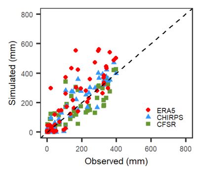
Remote Sens. 2021, 13, 3299                                                                                            9 of 20

                              3.4. Performance Evaluation of the Reanalysis Datasets and Simulated Streamflow
                                     Our aim was to qualitatively compare the ERA5, CHIRPS, and CFSR reanalysis
                              datasets with the rain gauge observations. The following statistical indices for validation
                              were used: the correlation coefficient (CC or R2 ), mean (M), standard deviation (SD),
                              mean error (ME), root-mean square error (RMSE), and relative bias (BIAS). The linear
                              correlation is indicated by CC, the average difference is shown by RMSE, and the average
                              error magnitude between the reanalysis precipitation and observed rain gauge data is
                              shown by ME. The systematic bias of the satellite precipitation is described by BIAS.
                                     Rainfall detection capability was analysed using three categorical statistical indices:
                              (1) the probability of detection (POD); (2) the false alarm rate (FAR); and (3) the critical
                              success index (CSI). The POD is also known as the hit rate. This is the ratio of total rainfall
                              events that are successfully recognised by the reanalysis datasets. The FAR indicates the
                              percentage of falsely warned rainfall events among all warnings. The most balanced and
                              accurate detection statistic is the CSI, which is a function of POD and FAR [58]. The POD,
                              FAR, and CSI scores range between 0 and 1, with 1 being a perfect score for POD and CSI
                              and 0 for FAR. The formulas and further details about the indices appear in Jiang et al.
                              (2018) [59].
                                     To assess the SWAT model’s accuracy, we included the coefficient of determination
                              (R2 ), the Nash–Sutcliffe efficiency ratio (NSE), percentage bias (PBIAS), observed data SD
                              ratio (RSR), and the Kling–Gupta efficiency ratio (KGE). These statistics are extensively
                              used in hydrological research [60]. At the monthly scale, when the PBIAS is below 25%
                              and the NSE and KGE are above 0.5, and the RSR is below 0.7, the model’s performance is
                              considered to be adequate [61,62].

                              4. Results and Discussion
                              4.1. Comparison between Observed and Reanalysis Datasets
                                   Precipitation data from the three reanalysis datasets (CFSR, ERA5, and CHIRPSv2.0)
                              were directly compared to precipitation data from rainfall stations in the GSM River Basin.
                              Daily precipitation data was collected from the reanalysis data grid cells closest to the
                              available weather stations; days with no observed data were omitted from the comparative
                              analysis. To enable conclusions regarding the flow simulation, we used the same period to
                              evaluate the accuracy of the precipitation data as the period for which the flow data was
                              available (2005–2010).
                                   The validation statistics for the GSM River Basin are presented in Table 3. Among
                              the three reanalysis datasets, the CHIRPS was more accurate; it yielded low ME values
                              together with higher CC and CSI values. Hence, it performed best in both accuracy and
                              detection capability. The results obtained from ERA5 and CFSR were also acceptable. In the
                              case of ERA5, the correlation with observed data was slightly lower than that yielded by
                              CHIRPS. Of the three reanalysis datasets, ERA5 achieved a monthly SD most similar to that
                              of the observed data. However, ERA5 presented the highest BIAS of the three reanalysis
                              datasets analysed, overestimating the rainfall values at some weather stations by more
                              than 40%. The higher amount of rainfall explained why ERA5 yielded relatively high POD
                              and FAR values.
                                   The CFSR yielded a smaller correlation with the observed data than CHIRPS and
                              ERA5. Conversely, the BIAS was lower than that shown by ERA5, which signified overesti-
                              mation or underestimation of the rainfall depending on the station analysed. The lower
                              BIAS value was related to a lower POD and FAR compared to the results obtained with
                              ERA5. On average, CSI was similar for both CFSR and ERA5, which implies a similar
                              detection capability.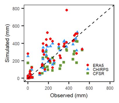
Remote Sens. 2021, 13, 3299                                                                                                                                                                          10 of 20

      Table 3. Comparison of various validation statistics for the different reanalysis products covering the GSM River Basin. Daily and monthly statistics are shown on the left and right sides of
      a/symbol. Gaps in gauge observation records result in different daily and monthly BIAS. Only months with complete daily data were compared.

     Station              Dataset            M                SD                 CC           RMSE (mm)           ME (mm)           BIAS (%)             POD               FAR                CSI
                         Observed          1469               274                 -                 -                 -                  -                 -                 -                  -
       MIG                ERA5             2105               303            0.43/0.85        13.54/115.23       6.04/72.05       38.32/40.60            0.91               0.50              0.48
                         CHIRPS            1752               285            0.52/0.93        10.71/61.44        4.55/41.87       13.33/15.69            0.79               0.35              0.54
                          CFSR             1441               356            0.27/0.84        12.91/71.01        5.70/51.54       −4.64/−4.75            0.79               0.48              0.44
                         Observed          1561               470                 -                 -                 -                  -                 -                 -                  -
       CHA                ERA5             2204               495            0.38/0.80        15.55/124.38       6.87/78.05        18.95/25.19           0.92               0.42              0.55
                         CHIRPS            1991               268            0.55/0.88        11.56/82.54        5.38/54.25        6.70/10.01            0.82               0.27              0.63
                          CFSR             1441               356            0.34/0.85        13.54/94.53        6.25/62.46       −21.73/−20.47          0.79               0.41              0.51
                         Observed          1136               731                 -                 -                 -                  -                 -                 -                  -
       DEL                ERA5             1994               549            0.49/0.83        14.33/123.69       5.97/82.61        46.89/48.62           0.89               0.53              0.45
                         CHIRPS            1821               341            0.62/0.86        11.13/97.85        5.06/63.11        31.66/33.74           0.80               0.40              0.52
                          CFSR             1817               385            0.38/0.86        13.56/92.77        5.97/65.00        27.86/30.30           0.89               0.54              0.43
                         Observed          1023               627                 -                 -                 -                  -                 -                 -                  -
        VIL               ERA5             2106               519            0.41/0.86        12.53/103.13       5.56/69.76        49.77/48.90           0.91               0.49              0.48
                         CHIRPS            1785               263            0.51/0.91         9.73/76.38        4.48/50.54        30.86/31.97           0.79               0.36              0.54
                          CFSR             1441               356            0.27/0.84        11.50/62.68        5.03/40.79        −0.07/0.78            0.75               0.48              0.44
Remote Sens. 2021, 13, 3299 11 of 19
Remote Sens. 2021, 13, 3299 11 of 20
Observed 1136 731 Figure 3-shows the probability
- density-function of rainfall
- events -on a daily- scale. -
It is evident that all the remote-sensing data we analysed missed some rain events and
ERA5 1994 549 0.49/0.83 14.33/123.69 5.97/82.61 46.89/48.62 0.89
CHIRPS was most similar to the observed data in this regard. ERA5 clearly overestimated
0.53 0.45
DEL
CHIRPS 1821 341amount
the 0.62/0.86 11.13/97.85
of light and medium rainfall5.06/63.11
events (where 31.66/33.74 0.80
‘light’ refers to 0.40 of0.52
daily rainfall
CFSR 1817 385mm) 0.38/0.86
1–5 and medium 13.56/92.77 5.97/65.00
refers to daily rainfall 27.86/30.30
of 5–20 mm). 0.89overestimating
CFSR, despite 0.54 0.43
Observed 1023 these
627 rainfall events,
- was the reanalysis
- dataset - that most closely
- reflected the
- observed
- data -
for medium rainfall events. Among the three reanalysis datasets, CHIRPS best represented
ERA5 2106 519 0.41/0.86 12.53/103.13 5.56/69.76 49.77/48.90 0.91 0.49 0.48
VIL light rainfall events, but it significantly overestimated medium rainfall events. Regarding
CHIRPS 1785 263 0.51/0.91 9.73/76.38 4.48/50.54 30.86/31.97 0.79 0.36
the highest intensity events (daily rainfall over 20 mm), the three reanalysis datasets yielded
0.54
CFSR 1441 356 performances.
similar 0.27/0.84 11.50/62.68 5.03/40.79 -0.07/0.78 0.75 0.48 0.44
FigureFigure 3. Description
3. Description of different
of different rainfall
rainfall intensitiesofofthe
intensities theprobability
probability density
densityfunction of of
function rainfall events
rainfall on aon
events daily scale.scale.
a daily
The general overestimation of the number of rainfall events and the volume of rainfall
As evident in Figure 4, monthly observed rainfall and variations in rainfall patterns
may be due to the ability of satellites to detect strong convective events while having more
were also analysed.
difficulty In the
in detecting left column,
shallow and warm violin
rains.plots combine
In addition, thebox
biasplots and atechniques
correction kernel density
plot to simultaneously represent the data distribution and probability density.
generally used to correct satellite data often inflate the volume of rainfall in the detected Except for
MIG, thetodensity
events distribution
compensate displayed
for the missed eventsa[63].
consistently more accurate adjustment when
using the AsCHIRPS
evident indata.
FigureThe4, median
monthly prediction
observed rainfall and as
is shown variations
a whitein rainfall
dot in thepatterns
graphs, and
were also analysed. In the left column, violin plots combine box plots and
significant differences were detected. In general, ERA5 overestimated the median value, a kernel density
plot to
except at simultaneously
the CHA station represent
(locatedtheat
data
thedistribution and probability
highest altitude), where density. Except for
the reanalysis data re-
MIG, the density distribution displayed a consistently more accurate adjustment when
sulted in an underestimated median value. Similarly, ERA5, CHIRPS and CFSR ade-
using the CHIRPS data. The median prediction is shown as a white dot in the graphs,
quately reflected the inter-annual variation in precipitation; they indicated the existence
and significant differences were detected. In general, ERA5 overestimated the median
of avalue,
dry period
except from
at theNovember
CHA station to(located
April and a wet
at the period
highest from May
altitude), where tothe
October.
reanalysis
A characteristic
data aspects of the climate
resulted in an underestimated medianin the study
value. areaERA5,
Similarly, is a maximum
CHIRPS and monthly
CFSR rain-
falladequately
that occurs between
reflected June andvariation
the inter-annual September, interrupted
in precipitation; theyby a typical
indicated mid-summer
the existence
of a dryduring
drought period the
frommonth
November to April
of July andThis
[36,64]. a wetpattern
period from
was May to October.
detected by all the products
we assessed. In addition, unlike CFSR, the ERA5 and CHIRPS datasets overestimated the
average monthly rainfall reported during the rainy season. We also found that the scat-
terplots suggested a higher performance for the CHIRPS data, with an overall closer fit
with the observations. This finding was supported by the calculated CC values. Using theRemote Sens. 2021, 13, 3299 12 of 19
Remote Sens. 2021, 13, 3299
contrast, for the CFSR and ERA5 datasets, the CC values ranged from 0.84 to 12 of 20
0.86 and 0.80
to 0.86, respectively.
MIG (−88.159, 13.439)
CHA (−88.260803, 13.6423998)
DEL (−88.1416016, 13.3274002)
VIL (−88.1794968, 13.5186996)
Figure 4. Comparison of average monthly observed precipitation with ERA5, CHIRTS, and CFSR datasets using violin
Figure 4. Comparison of average monthly observed precipitation with ERA5, CHIRTS, and CFSR datasets using violin
plots (left column), variations in rainfall patterns (central column) and scatterplots (right column).
plots (left column), variations in rainfall patterns (central column) and scatterplots (right column).
A characteristic aspects of the climate in the study area is a maximum monthly
The observed
rainfall that occursmonthly
betweentemperatures were interrupted
June and September, compared by to adata from
typical ERA5, CHIRTS
mid-summer
and drought
CFSR, as discussed
during in the
the month of previous section
July [36,64]. (Figure
This pattern 5).detected
was Although the
by all shape
the of the den-
products
we assessed. In addition, unlike CFSR, the ERA5 and CHIRPS datasets overestimated
sity distribution and the monthly variations showed a good fit, we noted a significant
overestimation of CHIRTS temperatures by 2–3 °C, depending on the month considered
over the year. For CFSR, an overestimation of the monthly mean temperature was also
detected for all months, which was far lower than that observed in CHIRTS. At the MIGRemote Sens. 2021, 13, 3299 13 of 20
the average monthly rainfall reported during the rainy season. We also found that the
scatterplots suggested a higher performance for the CHIRPS data, with an overall closer
fit with the observations. This finding was supported by the calculated CC values. Using
the CHIRPS data, the CC values for the tested weather stations ranged from 0.86 to 0.93.
By contrast, for the CFSR and ERA5 datasets, the CC values ranged from 0.84 to 0.86 and
0.80 to 0.86, respectively.
The observed monthly temperatures were compared to data from ERA5, CHIRTS,
and CFSR, as discussed in the previous section (Figure 5). Although the shape of the
Remote Sens. 2021, 13, 3299 density distribution and the monthly variations showed a good fit, we noted a significant 13 of 19
overestimation of CHIRTS temperatures by 2–3 ◦ C, depending on the month considered,
over the year. For CFSR, an overestimation of the monthly mean temperature was also
detected for all months, which was far lower than that observed in CHIRTS. At the MIG
station, which was the only station for which temperature data was available, the data
station, which was the only station for which temperature data was available, the data
fromfrom
ERA5ERA5provided
provided the
thebest
bestfit.
fit.
MIG (−88.159, 13.439)
5. Comparison of average monthly observed temperature with ERA5, CHIRTS, and CFSR datasets using violin plots
Figure 5.Figure
Comparison of average monthly observed temperature with ERA5, CHIRTS, and CFSR datasets using violin
(left column), variations in rainfall patterns (central column) and scatterplots (right column).
plots (left column), variations in rainfall patterns (central column) and scatterplots (right column).
4.2. Model Performance before Calibration
4.2. ModelWhen
Performance before Calibration
data is missing from observations, the performance of an uncalibrated model
When
is data is missing
an important indicator from
of how observations,
well the model theperforms
performance
[65]. Theof main
an uncalibrated
purpose for model
which the SWAT model was conceived was to model ungauged
is an important indicator of how well the model performs [65]. The main rural watersheds [10].purpose
The for
suitability of the different reanalysis datasets was evaluated by simulating
which the SWAT model was conceived was to model ungauged rural watersheds [10]. flows within the
SWAT model framework using default parameters.
The suitability of the different reanalysis datasets was evaluated by simulating flows
Figure 6 shows the observed and simulated monthly runoff in the GSM River Basin for
within
thethe SWAT
period modelThe
2005–2010. framework
criteria forusing default
evaluating the parameters.
model performance are indicated in
Figure5,6from
Figure shows theit observed
which andCFSR
is evident that simulated
yielded monthly runoff
the best results. in was
This the asGSM River Basin
expected,
for the period
since 2005–2010.
this dataset The criteria
contained the leastfor evaluating
biased reanalysisthe model
data. performance
However, are indicated
it is important
to note5,that
in Figure fromon awhich
monthly scale,
it is all thethat
evident reanalysis
CFSR datasets
yieldedyielded
the best adequate
results.CCs, which
This was as ex-
ranged between 0.64 and 0.74. These results suggest that after calibrating the most sensitive
pected, since this dataset contained the least biased reanalysis data. However, it is im-
parameters, the overall performance of the models may be acceptable.
portant to note that on a monthly scale, all the reanalysis datasets yielded adequate CCs,
which ranged between 0.64 and 0.74. These results suggest that after calibrating the most
sensitive parameters, the overall performance of the models may be acceptable.Figure 6 shows the observed and simulated monthly runoff in the GSM River Basin
for the period 2005–2010. The criteria for evaluating the model performance are indicated
in Figure 5, from which it is evident that CFSR yielded the best results. This was as ex-
pected, since this dataset contained the least biased reanalysis data. However, it is im-
portant to note that on a monthly scale, all the reanalysis datasets yielded adequate CCs,
Remote Sens. 2021, 13, 3299 14 of 20
which ranged between 0.64 and 0.74. These results suggest that after calibrating the most
sensitive parameters, the overall performance of the models may be acceptable.
Figure6.6. Model
Figure Model performance
performance comparison
comparison for
for the
the default
default SWAT
SWATmodel
modelusing
usingERA5,
ERA5,CHIRPS-CHIRTS,
CHIRPS-CHIRTS,and
andCFSR
CFSRdatasets
datasets
for the input data together with monthly observed streamflows.
for the input data together with monthly observed streamflows.
4.3.
4.3. Model
Model Calibration
Calibration Using
Using GLoFAS
GLoFASDischarge
DischargeData
Data
As
As shown in Figure 2, we first compared the observed
shown in Figure 2, we first compared the observed rainfall
rainfall and
and temperature
temperaturedata
data
and
and the reanalysis data. Then we evaluated the performance of three datasets as
the reanalysis data. Then we evaluated the performance of three datasets as inputs
inputs
for
for the SWAT model
the SWAT model totosimulate
simulatethetheobserved
observedflow
flowinin
thethe GSM
GSM River
River Basin.
Basin. For pur-
For this this
purpose, the SWAT model was calibrated for each of the reanalysis products,
pose, the SWAT model was calibrated for each of the reanalysis products, including both including
both precipitation
precipitation and temperature.
and temperature. The SUFI-2
The SUFI-2 algorithmalgorithm
includedincluded in the SWATCUP
in the SWATCUP software
software was used to optimise 12 SWAT parameters. Parameter selection was based on
previous studies in nearby catchments in El Salvador [36], as mentioned in Section 3.3.
In addition, a sensitivity analysis was conducted to determine the most sensitive
parameters using each of the reanalysis datasets as input data and performing 500 model
runs. As shown in Table 3, regardless of the reanalysis data used, CN2 was the most
sensitive parameter, followed by GWQMN and ESCO; these parameters obtained the
lowest p-values. The p-value for each parameter represents a test of the null hypothesis
that the regression coefficient is equal to zero. According to Abbaspour et al. (2007) [66],
the more sensitive the parameter, the smaller the p-value.
Table 4 shows the parameter ranges and the final calibrated values for each of the
reanalysis products. Among the calibrated parameters—and as demonstrated by the
sensitivity analysis, CN2 was one of the most sensitive parameters as it is directly related
to runoff generation [67,68]. We thus expected that the calibrated CN2 values would be
substantially reduced to correct the overestimation of precipitation as detected using the
reanalysis data, with the expected reduction being between 11.7% and 19.9%.
Table 4. Calibrated parameter values.
Calibrated Value
Parameter Range
ERA5 CHIRPS-CHIRTS CFSR
CN2.mgt −0.2 to 0.2 −0.199 −0.117 −0.157
ALPHA_BF.gw 0.01 to 1 0.85555 0.5099 0.24333
GWQMN.gw 0 to 5000 4765 3675 195
GW_REVAP.gw 0.02 to 0.2 0.1167 0.1026 0.0846
RCHRG_DP.gw 0 to 1 0.315 0.065 0.785
REVAPMN.gw 0 to 500 356.5 302.5 320.5
CANMX.hru 0 to 100 90.9 95.7 29.5
EPCO.bsn 0 to 1 0.499 0.819 0.365
ESCO.bsn 0 to 1 0.8155 0.801 0.861
SOL_AWC.sol −0.3 to 0.3 0.055 −0.1974 −0.213
LAT_TTIME.hru 0 to 180 48.06 108.90 15.3
SLSOIL.hru 0 to 150 43.35 38.55 35.25Remote Sens. 2021, 13, 3299 15 of 20
Remote Sens. 2021, 13, 3299 15 of 19
In addition, ESCO was also reduced from the default value of 0.95 to values between
Table
0.805.and
SWAT
0.86,model
whichperformance
represents ancompared with
increase in GloFAS discharge
evaporation generateddata.
by the model. These
ESCO values are in line with those obtained in other tropical areas [36,69]. The largest
Dataset data were noted for the ground-
discrepancies between the fitted values and the reanalysis
Parameter ERA5 GWQMN, GW_REVAP,
water parameters (ALPHA_BF, CHIRPS-CHIRTS RCHRG_DP and REVAPMN). CFSRThis
result might be attributable
Calibration to the inherent
Validation complexity Validation
Calibration of the volcanicCalibration
aquifers in Central
Validation
America;
R 2 the aquifers
0.88 display high
0.82 permeability
0.78 and fissure
0.78 flows, making
0.82 them very0.60
complicated to study [70]. However, ALPHA_BF varied from 0.24 (for CFSR) to 0.85 (for
NSE 0.87 0.81 0.77 0.70 0.81
ERA5). The latter value indicates a faster recharge response [71], which is consistent with
0.54
PBIAS (%) −11.68 −13.36
the volcanic aquifers in the study area. 7.34 −30.70 −3.29 −32.31
KGEThe performance
0.86 of the calibrated
0.81 model0.85
for each of the0.65
input datasets0.88
is summarised 0.47
in Table 5. The statistics show that the SWAT model simulated the GloFAS discharge flows
4.4.reasonably
Evaluationwell forSimulated
of the both calibration
Monthly(2005–2008) and validation
Streamflows for Various(2009–2010)
Scenarios periods. This
result was independent of the reanalysis data, since all the simulations had a CC ranging
Finally,
between the
0.76 simulated
and monthly
0.85, an NSE greater scale flows
than 0.50, andobtained
a KGE value from the GloFAS
between 0.84 and calibration
0.86.
were compared
As expected, thewith the observed
best results flows.
were obtained The
using simulations
data from ERA5, performed
which is usedusing CHIRPS-
to obtain
CHIRTS data showed
the global-scale flowsthe best fit, as evident in Figure 7. Nonetheless, all three simulations
in GloFAS.
performed using ERA5, CHIRPS-CHIRTS, and CFSR data showed an acceptable fit with
theTable 5. SWAT
observed model performance compared with GloFAS discharge data.
streamflows.
These results demonstrate that when theDataset ERA5 reanalysis data show an adequate fit,
GloFAS discharge
Parameter data could
ERA5 potentially be used
CHIRPS-CHIRTSto simulate the hydrological
CFSR processes
of ungauged catchments at the monthly scale. This would allow the use of distributed
Calibration Validation Calibration Validation Calibration Validation
hydrological models such as SWAT to analyse fundamental aspects in water resource
R2 0.88 0.82 0.78 0.78 0.82 0.60
management—such
NSE 0.87as the impact
0.81 of changes
0.77 in land 0.70use or the
0.81climate. Similar
0.54 to our
findings,
PBIASEini
(%) et −al.11.68
(2019) [72] reported 7.34
−13.36 that when−30.70precipitation
−3.29 reanalysis data repre-
−32.31
sented KGE
well-observed 0.86 precipitation
0.81 0.85 than 0.6)
(R2 higher 0.65 in a semi-arid
0.88 0.47in Iran, the
basin
result was reasonable simulations for river discharge. However, these results should be
4.4. Evaluation
viewed of the Simulated
with caution Monthly Streamflows
as they depend for Various
on the quality of theScenarios
GloFAS adjustment to the ob-
served Finally, thethis
flows. In simulated
regard,monthly scale
Harrigan flows
et al. obtained
(2020) from the GloFAS
[30] demonstrated calibration
that the quality of
were compared with the observed flows. The simulations performed using
the GloFAS adjustment increased substantially along with the size of the catchment. We CHIRPS-
CHIRTS data showed the best fit, as evident in Figure 7. Nonetheless, all three simulations
thus recommend that the methodology followed in our study should be replicated in
performed using ERA5, CHIRPS-CHIRTS, and CFSR data showed an acceptable fit with
larger catchments.
the observed streamflows.
FigureFigure 7. Model
7. Model performance
performance comparison
comparison betweensimulated
between simulated and
andobserved
observedmonthly
monthlystreamflows after after
streamflows calibration using using
calibration
GLoFAS discharge
GLoFAS discharge data. data.
4.5. Limitations and Future Research Directions
This study demonstrates that when remotely sensed weather data are accurate with
respect to observed climatological data, flow simulation is often accurate. Hence, the use
of discharge data, such as GLoFAS, contributes to the correct simulation of the hydrolog-
ical processes in a basin. However, several limitations need to be considered. Firstly, dataRemote Sens. 2021, 13, 3299 16 of 20
These results demonstrate that when the ERA5 reanalysis data show an adequate fit,
GloFAS discharge data could potentially be used to simulate the hydrological processes
of ungauged catchments at the monthly scale. This would allow the use of distributed
hydrological models such as SWAT to analyse fundamental aspects in water resource
management—such as the impact of changes in land use or the climate. Similar to our
findings, Eini et al. (2019) [72] reported that when precipitation reanalysis data represented
well-observed precipitation (R2 higher than 0.6) in a semi-arid basin in Iran, the result
was reasonable simulations for river discharge. However, these results should be viewed
with caution as they depend on the quality of the GloFAS adjustment to the observed
flows. In this regard, Harrigan et al. (2020) [30] demonstrated that the quality of the
GloFAS adjustment increased substantially along with the size of the catchment. We
thus recommend that the methodology followed in our study should be replicated in
larger catchments.
4.5. Limitations and Future Research Directions
This study demonstrates that when remotely sensed weather data are accurate with
respect to observed climatological data, flow simulation is often accurate. Hence, the use of
discharge data, such as GLoFAS, contributes to the correct simulation of the hydrological
processes in a basin. However, several limitations need to be considered. Firstly, data from
a single flow-gauging station at the outlet of the basin was used to calibrate the model. This
means there is the possibility of equifinality issues with some parameters having optimal
values that are physically unrealistic. Future research should include additional calibration
with other variables that are available through remote sensing, such as evapotranspiration.
Second, NSE has been used as the objective function. This coefficient usually presents
the problem of being weighted towards higher flows. The use of other objective functions
would return different results, and it would be interesting to study the effect of the selected
objective function on the results obtained.
Third, only the SWAT model was employed to test the methodological approach used
in this work. Future research and performance testing with different hydrological models
could help to clarify the limitations and strengths of our methodological approach. Finally,
if observed data is available, future studies could assess the performance of GLoFAS
discharge data on a daily and sub-daily basis.
5. Conclusions
This study evaluates the application of GLoFAS discharge data in model calibration
in El Salvador, Central America. This is a country in which climatological input data and
observed flow data for calibrating hydrological models is scarce or unavailable. GLoFAS
determines the streamflow by applying a global-scale hydrological model that uses ERA5
reanalysis data as the input data. This work tested whether the streamflow data from
GLoFAS provided a suitable option for calibrating hydrological models in ungauged
catchments, as long as there is a good fit between reanalysis precipitation and temperature
data and observed climatological data. Climatological reanalysis data (CHIRPS-CHIRTS
and CFSR) were also evaluated. The following conclusions are presented:
(1) The statistical indicators (CC, RMSE, ME, and BIAS) allowed the accuracy of the
reanalysis data to be quantitatively evaluated. We found that CHIRPS performed
best in reproducing the observed precipitation, despite consistently overestimating
the rainfall.
(2) In terms of rain detection ability, CHIRPS (CSI ranging from 0.52 to 0.63) displayed
the greatest daily accuracy in detecting the precipitation occurrences. The next best
were ERA5 and then CFSR. However, all three reanalysis datasets showed acceptable
rainfall detection capability.
(3) Among the three temperature reanalysis products, the performance of CHIRTS was
the least accurate; it repeatedly overestimated mean temperature by 2–3 ◦ C. By
contrast, ERA5 and CFSR presented excellent agreement with the observed data.Remote Sens. 2021, 13, 3299 17 of 20
(4) Models that were calibrated using GloFAS data as the observed data, independently of
the precipitation and temperature data (ERA5, CHIRPS-CHIRTS and CFSR) showed
acceptable model performance. This point was evident in the KGE values, which
ranged from 0.74 to 0.79, and the R2 values of between 0.57 and 0.78.
Overall, these findings demonstrate that reanalysis rainfall products can improve
hydrological process modelling for Central American watersheds, where poorly gauged or
ungauged watersheds are common. This research also highlights the GLoFAS dataset’s
potential for model calibration in catchments where the availability of streamflow data is
limited. The availability of a calibrated hydrological model that adequately reflects the
hydrological processes of a basin provides decision-makers with a tool to quantify the
availability of water resources. The modelalso provides the basis for estimating the impact
of land use changes or climate change on water resources.
Author Contributions: J.S.-A. and P.B.-G. conceived and designed the experiments; P.B.-G., P.J.-S. and
A.L.-B. performed the experiments and analysed the data; J.P.-S. provided reviews and suggestions;
J.S.-A. prepared the manuscript with contributions from all co-authors. All authors have read and
agreed to the published version of the manuscript.
Funding: This research was funded by the European Union’s Horizon 2020 research and
innovation programme within the framework of the project SMARTLAGOON, grant agreement
number 101017861.
Acknowledgments: The authors acknowledge Scribbr editing services for proofreading the manuscript.
Conflicts of Interest: The authors declare no conflict of interest.
References
1. Kiros, G.; Shetty, A.; Nandagiri, L. Performance evaluation of SWAT model for land use and land cover changes under different
climatic conditions: A review. J. Waste Water Treat. Anal. 2015, 6, 1–6. [CrossRef]
2. Krysanova, V.; Srinivasan, R. Assessment of climate and land use change impacts with SWAT. Reg. Environ. Chang. 2014, 15,
431–434. [CrossRef]
3. Kok, K.; Winograd, M. Modelling land-use change for Central America, with special reference to the impact of hurricane mitch.
Ecol. Model. 2002, 149, 53–69. [CrossRef]
4. Hidalgo, H.G.; Amador, J.A.; Alfaro, E.J.; Quesada, B. Hydrological climate change projections for Central America. J. Hydrol.
2013, 495, 94–112. [CrossRef]
5. Srivastava, A.; Sahoo, B.; Raghuwanshi, N.S.; Singh, R. Evaluation of variable-infiltration capacity model and modis-terra
satellite-derived grid-scale evapotranspiration estimates in a river basin with tropical monsoon-type climatology. J. Irrig. Drain.
Eng. 2017, 143, 04017028. [CrossRef]
6. Srivastava, A.; Deb, P.; Kumari, N. Multi-Model approach to assess the dynamics of hydrologic components in a tropical
ecosystem. Water Resour. Manag. 2020, 34, 327–341. [CrossRef]
7. Paul, P.K.; Kumari, N.; Panigrahi, N.; Mishra, A.; Singh, R. Implementation of cell-to-cell routing scheme in a large scale
conceptual hydrological model. Environ. Model. Softw. 2018, 101, 23–33. [CrossRef]
8. Fukunaga, D.C.; Cecílio, R.; Zanetti, S.S.; Oliveira, L.T.; Caiado, M.A.C. Application of the SWAT hydrologic model to a tropical
watershed at Brazil. Catena 2015, 125, 206–213. [CrossRef]
9. Darbandsari, P.; Coulibaly, P. Inter-comparison of lumped hydrological models in data-scarce watersheds using different
precipitation forcing data sets: Case study of Northern Ontario, Canada. J. Hydrol. Reg. Stud. 2020, 31, 100730. [CrossRef]
10. Arnold, J.G.; Srinivasan, R.; Muttiah, R.S.; Williams, J.R. Large area hydrologic modeling and assessment part I: Model develop-
ment. JAWRA J. Am. Water Resour. Assoc. 1998, 34, 73–89. [CrossRef]
11. Abbaspour, K.C.; Vaghefi, S.A.; Yang, H.; Srinivasan, R. Global soil, landuse, evapotranspiration, historical and future weather
databases for SWAT Applications. Sci. Data 2019, 6, 1–11. [CrossRef] [PubMed]
12. Hughes, D.A. Comparison of satellite rainfall data with observations from gauging station networks. J. Hydrol. 2006, 327, 399–410.
[CrossRef]
13. Tan, M.L.; Yang, X. Effect of rainfall station density, distribution and missing values on SWAT outputs in tropical region. J. Hydrol.
2020, 584, 124660. [CrossRef]
14. Dhanesh, Y.; Bindhu, V.; Senent-Aparicio, J.; Brighenti, T.; Ayana, E.; Smitha, P.; Fei, C.; Srinivasan, R. A comparative evaluation
of the performance of CHIRPS and CFSR data for different climate zones using the SWAT model. Remote Sens. 2020, 12, 3088.
[CrossRef]
15. Mazzoleni, M.; Brandimarte, L.; Amaranto, A. Evaluating precipitation datasets for large-scale distributed hydrological modelling.
J. Hydrol. 2019, 578, 124076. [CrossRef]You can also read