Evaluation of ECMWF IFS-AER (CAMS) operational forecasts during cycle 41r1-46r1 with calibrated ceilometer profiles over Germany
←
→
Page content transcription
If your browser does not render page correctly, please read the page content below
Geosci. Model Dev., 14, 1721–1751, 2021
https://doi.org/10.5194/gmd-14-1721-2021
© Author(s) 2021. This work is distributed under
the Creative Commons Attribution 4.0 License.

Evaluation of ECMWF IFS-AER (CAMS) operational forecasts
during cycle 41r1–46r1 with calibrated ceilometer
profiles over Germany
Harald Flentje1 , Ina Mattis1 , Zak Kipling2 , Samuel Rémy3 , and Werner Thomas1
1 Deutscher
         Wetterdienst, Met. Obs. Hohenpeißenberg, Albin-Schwaiger-Weg 10, Hohenpeißenberg, Germany
2 European
        Centre for Medium-Range Weather Forecasts, Shinfield Park, Reading, UK
3 HYGEOS, 165 Avenue de Bretagne, Lille, France

Correspondence: Harald Flentje (harald.flentje@dwd.de)

Received: 11 September 2020 – Discussion started: 7 October 2020
Revised: 27 January 2021 – Accepted: 2 February 2021 – Published: 29 March 2021

Abstract. Aerosol forecasts by the European Centre for             ues from Saharan dust and sea salt are considerably overes-
Medium-Range Weather Forecasts (ECMWF) Integrated                  timated. Differences between model and ceilometer profiles
Forecasting System aerosol module (IFS-AER) for the years          are investigated using observed in situ mass concentrations
2016–2019 (cycles 41r1–46r1) are compared to vertical pro-         of organic matter (OM), black carbon, SO4 , NO3 , NH4 and
files of particle backscatter from the Deutscher Wetterdienst      proxies for mineral dust and sea salt near the surface. Ac-
(DWD) ceilometer network. The system has been developed            cordingly, SO4 and OM sources as well as gas-to-particle
in the Copernicus Atmosphere Monitoring Service (CAMS)             partitioning of the NO3 –NH4 system are too strong. The top
and its precursors. The focus of this article is to evaluate the   of the mixing layer on average appears too smooth and sev-
realism of the vertical aerosol distribution from 0.4 to 8 km      eral hundred meters too low in the model. Finally, a dis-
above ground, coded in the shape, bias and temporal varia-         cussion is included of the considerable uncertainties in the
tion of the profiles. The common physical quantity, the atten-     observations as well as the conversion from modeled to ob-
uated backscatter β ∗ (z), is directly measured and calculated     served physical quantities and from necessary adaptions of
from the model mass mixing ratios of the different particle        varying resolutions and definitions.
types using the model’s inherent aerosol microphysical prop-
erties.
   Pearson correlation coefficients of daily average simulated
and observed vertical profiles between r = 0.6–0.8 in sum-         1   Introduction
mer and 0.7–0.95 in winter indicate that most of the verti-
cal structure is captured. It is governed by larger β ∗ (z) in     Aerosol particles play a key role in atmospheric processes,
the mixing layer and comparably well captured with the suc-        and their manifold sources and transformations reflect in a
cessive model versions. The aerosol load tends to be biased        wide range of abundance as well as chemical and physi-
high near the surface, underestimated in the mixing layer and      cal properties. Thus, the understanding of particles’ net ef-
realistic at small background values in the undisturbed free       fects on air quality, weather, climate and chemical budgets
troposphere. A seasonal cycle of the bias below 1 km height        still comprises significant uncertainties (Linares et al., 2009;
indicates that aerosol sources and/or lifetimes are overesti-      WMO, 2013; Baklanov et al., 2014). Particles affect cli-
mated in summer and pollution episodes are not fully re-           mate and weather directly by light scattering and absorption
solved in winter. Long-range transport of Saharan dust or fire     (Hansen et al., 1997; Ramanathan et al., 2007; WMO, 2013)
smoke is captured and timely, only the dispersion to smaller       and indirectly by altering the formation and droplet size of
scales is not resolved in detail. Over Germany, β ∗ (z) val-       clouds (Lohmann et al., 2007) and via their impact on satu-
                                                                   ration and vertical exchange (Ackerman et al., 2000). Due to

Published by Copernicus Publications on behalf of the European Geosciences Union.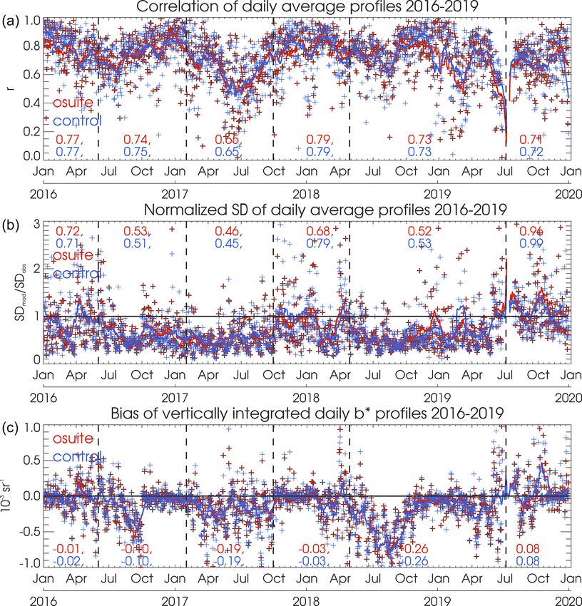
1722                                                                        H. Flentje et al.: CAMS aerosol profile evaluation

land-use changes and increasing emissions of anthropogenic          the Copernicus Atmosphere Monitoring Service (CAMS;
gases and particles during the last century, aerosols consti-       https://atmosphere.copernicus.eu/charts/cams/, last access:
tute and trigger severe pollution episodes and health haz-          25 March 2021) at the European Centre for Medium-Range
ards (Galanter et al., 2000; Andreae and Merlet, 2001; Pérez        Weather Forecasts (ECMWF) (Morcrette et al., 2009; Flem-
et al., 2012). In the lower troposphere, particle emissions and     ming et al., 2017; Rémy et al., 2019). Significant progress has
heterogeneous chemical processes degrade health-related air         been made with emission inventories (Granier et al., 2011;
quality (Gilge et al., 2010; Karanasiou et al., 2012), but at the   EDGAR, 2013; Gidden et al., 2019), implemented source
same time particles mediate gas-to-particle conversion, scav-       functions (Dentener et al., 2006; Morcrette et al., 2009, 2011;
enging and final removal of trace gases from the atmosphere         Spracklen et al., 2011) and the data assimilation (Benedetti
(Birmili et al., 2003; Kolb and et al, 2010).                       et al., 2009; Kaiser et al., 2012; Bocquet et al., 2015). Impor-
   Natural particle sources, too, dependent on season,              tant processes like water uptake and release by hygroscopic
weather and region, may cause widespread socio-economical           fractions (Weingartner et al., 2002; Swietlicki et al., 2008;
and epidemiological impacts. Europe, for example, is                Hong et al., 2014; Chan et al., 2018) have been included,
reached by Saharan dust (SD) many times per year (Ans-              while the extension to water cloud formation, e.g., during
mann and et al, 2003; Collaud-Coen et al., 2004; Papayannis         dust events, is still missing, though it regularly causes no-
et al., 2008; Pey et al., 2013; Flentje et al., 2015) where, de-    ticeable prediction errors.
creasing towards the north, it contributes between 5 %–30 %            It is therefore essential to evaluate and improve the CAMS
to the total dry particle mass (Putaud et al., 2010). It trig-      model system with the aid of independent observations,
gers cloud formation (Sassen et al., 2003; Lohmann et al.,          which is the mandate of (amongst others) the CAMS-84
2007; Tegen and Schepanski, 2009) and summer smog (Or-              validation team (Eskes et al., 2015). So far, model evalua-
donez et al., 2010; Wang, 2010) and has been associated with        tion concentrates on aerosol optical depth (AOD) (Holben
dispersion of bacteria like meningitis (Griffin, 2007; Karana-      et al., 2001; Basart et al., 2012; Cesnulyte et al., 2014); how-
siou et al., 2012). Volcanic eruptions may induce long-term         ever, this is limited to daytime (except a few moon radiome-
changes of radiation transfer (Jäger, 2005), disturb flight traf-   ters) and without resolving the vertical distribution. Regional
fic (Flentje et al., 2010a; Schumann et al., 2011) and habit-       models mostly think and verify in terms of particulate mat-
ability of adjacent regions and alter the chemical balance up       ter mass concentration (PM10 or PM2.5 ), mostly without re-
to the stratosphere. Domestic heating and open fires linked         solving composition and sizes of particles (Stidworthy et al.,
to agriculture (∼ 85 % globally; Andreae and Merlet, 2001),         2018; Akritidis et al., 2018). Often, assessments of detailed
drought or boreal burns (Damoah et al., 2004; Hyer et al.,          particle properties suffer from sparse or delayed observa-
2007; Stohl et al., 2002) produce small-sized carbonaceous          tions, which however are already used to verify CAMS re-
particles which can be widely distributed and may pene-             analyses (Flemming et al., 2017; Inness et al., 2019), which
trate deep into lungs and plant stomata (Kaiser et al., 2012).      use nearly the same aerosol module. Only recently, evalua-
Their fractal surfaces favor adsorption of harmful combus-          tion of vertical aerosol profiles started using research lidars
tion byproducts that may cause respiratory, allergic, cardio-       and ceilometers (Benedetti et al., 2009; Wiegner and Geiß,
vascular and cancerous diseases (Mölter et al., 2014).              2012; Wiegner et al., 2014; Chan et al., 2018), whereby the
   Air-quality regulations like European directive                  former are operated spatially sparse and temporally inter-
2008/50/EG for PM10 / PM2.5 have therefore been en-                 mittent, the latter have no independent capability to iden-
forced and are currently revised to tackle issues related           tify and quantify particles, and both at best capture part of
to carbonaceous fine (PM1 ) and ultrafine (< 0.1 µm) par-           the surface layer. Yet, extended networks like the European
ticles (Linares et al., 2009). Design and control of these          Aerosol Research Lidar Network (EARLINET), the German
legislations require modeling efforts to define their scope,        (Ceilonet) and the European (E-PROFILE) ceilometer net-
identify critical parameters and monitor the abundance of           works (cf. Global Aerosol Lidar Network (GALION), World
aerosols and their role in weather, climate and air quality         Meteorological Organization – Global Atmosphere Watch
(Stier et al., 2005; Morcrette et al., 2009; Grell et al., 2011;    (WMO-GAW) Report No. 178) are now in place and used.
Wang et al., 2011; Zhang et al., 2012; Baklanov et al., 2014).      As a byproduct, the height of the mixing layer (ML) can
Still the impacts on regional weather by mineral dust (Pérez        be inferred from the profiles (Münkel et al., 2007; Haeffelin
et al., 2006), sea salt (precursors) (O’Dowd et al., 1997) and      et al., 2012), which is used by aerosol and chemistry trans-
forest-fire particles (Andreae and Merlet, 2001; Stohl et al.,      port models to constrain the vertical exchange and to scale
2002; Andreae and Rosenfeld, 2008)) are a challenge for             the dispersion of reactive gases and aerosols (Monks et al.,
atmospheric models due to uncertainties of optical properties       2009) as well as greenhouse gas concentration budgets (Ger-
arising from assumptions on their physical and chemical             big et al., 2008).
composition (Curci et al., 2015).                                      The general approach in this article builds on the work
   To this end, the Integrated Forecasting System (IFS) for         of Chan et al. (2018) but allows us to investigate addi-
regional and global scales has been developed in the se-            tional model details beyond those discussed in there and
ries of PROMOTE, GEMS, MACC I–III EU projects for                   complements Flemming et al. (2017), Rémy et al. (2019).

Geosci. Model Dev., 14, 1721–1751, 2021                                             https://doi.org/10.5194/gmd-14-1721-2021
H. Flentje et al.: CAMS aerosol profile evaluation 1723
We primarily use attenuated backscatter β ∗ (z) profiles from Global Fire Assimilation System (GFAS) (Kaiser et al.,
the German ceilometer network to evaluate CAMS global 2012), or they are calculated from the meteorological fields
aerosol model forecasts. After brief overviews of the CAMS and surface conditions for dust, sea salt and biogenic parti-
model and potential and limitations of the ceilometer data, cles. Volcanic emissions can be activated on demand. Hori-
we introduce the auxiliary data aiding the interpretation as zontal and vertical transport is based on the dynamics of the
well as the concept and metrics to categorize the results in ECMWF model, complemented by vertical diffusion or con-
Sect. 2. The results (Sect. 3) present complementary ways vection, sedimentation and dry or wet deposition by large-
to order the model–observation differences occurring with scale and convective precipitation. The most significant up-
respect to altitude, time and model configuration. Based on grades are the increase of horizontal resolution from T255 to
this, we identify reasons for model deficiencies, possible im- T511 after June 2016, the switch to MACCity+SOA cou-
provements and parallels to previous evaluations in Sect. 4. pling OM to CO emission (Spracklen et al., 2011) as of
Key findings are summarized and an outlook is provided for February 2017, the increase of vertical resolution from 60
upcoming activities in Sect. 5. to 137 levels and the addition of NO3 and NH4 as of cycle
46r1 in July 2019; cf. Table 3 in Rémy et al. (2019).
Based on the 00:00 UTC analysis, 3-hourly profiles at
2 Data sets and methodology time steps of +3, +6, +9, . . ., +24 h are extracted from 5 d
forecast runs, making noticeable adaptations by the anal-
2.1 The CAMS aerosol model ysis/assimilation possible at 03:00 UTC each. Ceilometer
and model profiles as well as mixing layer height (MLH)
The IFS aerosol module (IFS-AER) is described in Benedetti are based on altitude above ground and model geopotential
et al. (2009), Morcrette et al. (2009) and Rémy et al. (2019). height, respectively. The vertical displacement between the
Further information as well as analyses, forecasts, eval- low-resolved model orography and real terrain height is only
uation results and other products can be found at https: relevant for steep stations sticking out far above the model
//atmosphere.copernicus.eu/ (last access: 25 March 2021). surface level, while over flat terrain this is below 100 m. In or-
This article refers to the operational runs with assimilation der to translate the model state of the atmosphere into virtual
(ASM) from January 2016 (cycle 41r1) to December 2019 measurements, which can be directly compared to real obser-
(cycle 46r1) and corresponding unconstrained control runs vations, a so-called “forward operator” is applied to the IFS-
(CTR) as listed in Table 1 and in Table 3 in Rémy et al. AER output. Here, the forward operator converts the mass
(2019). The data were resampled from the reduced Gaus- mixing ratios mp,i of 14 particle types to attenuated backscat-
sian grid at T255 spectral resolution to 1.0◦ × 1.0◦ before ter β ∗ (z) according to Eq. (1). This is chosen as a common
June 2016 and from T511 to 0.5◦ × 0.5◦ thereafter. Concep- physical quantity rather than backscatter coefficients β(z) be-
tually, regional models build on the global forecasts and re- cause it is the primary measured variable from ceilometers
fine scales to a few kilometers but yet provide only aggre- without assumptions involved, and the model contains all in-
gated aerosol quantities (PM2.5 or PM10 ) rather than spe- formation to calculate it:
ciated or direct backscatter output nor the information nec-
essary for conversion. The global aerosol model uses 14 Zz
β ∗ (z) = β(z) exp −2 σ (z0 )dz0 . (1)
prognostic variables: three size bins each of dust and sea
salt, hydrophilic/hydrophobic black carbon (BC), organic 0
matter (OM), sulfate (SO4 ) and, as of 9 July 2019 (cycle Here, β(z) and σ (z) are the backscatter and extinction coef-
46r1), also two size bins of nitrate (NO3 ) and ammonium ficients, respectively. The further procedure as described in
(NH4 ). MODIS AOD and, starting from cycle 45r1, the Po- detail by Chan et al. (2018) and look-up tables with conver-
lar Multi-sensor Aerosol product (Popp, 2016) are assimi- sion coefficients are in Appendices A and C, respectively.
lated, optionally by 4D-Var (Benedetti et al., 2009) or the
3-D fields from the previous forecast. Due to an adverse ef- 2.2 Ceilometer network
fect on headline scores during tests with Cloud-Aerosol Li-
dar with Orthogonal Polarization (CALIOP) backscatter pro- The German Meteorological Agency (Deutscher Wetterdi-
files (1D-Var), no aerosol profiles have been assimilated yet enst; DWD) operates a network of about 160 Lufft-CHM15k
(Benedetti et al., 2009). As described in detail by Granier ceilometers (∼ 60 in January 2016; Fig. 1) which pro-
et al. (2011), EDGAR (2013) and Rémy et al. (2019) and vide operational profiles of the background- and range-
documented on the ECMWF website (https://confluence. corrected raw signal P (z)z2 (Flentje et al., 2010a, b), avail-
ecmwf.int/display/COPSRV/CAMS+Global/, last access: able as QuickLooks at http://www.dwd.de/ceilomap/ (last
25 March 2021), aerosol sources in IFS-AER con- access: 25 March 2021) and the European E-PROFILE
tinuously develop with emission inventories EDGAR, (https://ceilometer.e-profile.eu/, last access: 25 March 2021).
MACCity(+SOA), CAMS_GLOB_ANT/BIO vx.x (anthro- CHM15k uses a diode-pumped Nd:YAG solid-state laser
pogenic/biogenic), stem from scaled fire emissions of the emitting at 1064 nm and ranges up to maximum 15 km above
https://doi.org/10.5194/gmd-14-1721-2021 Geosci. Model Dev., 14, 1721–1751, 2021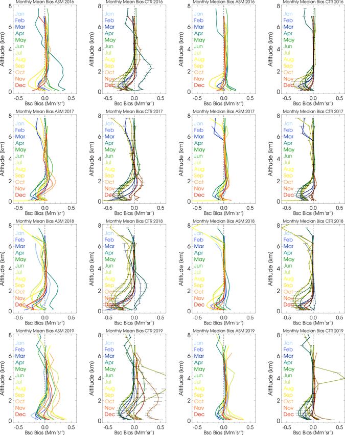
1724                                                                              H. Flentje et al.: CAMS aerosol profile evaluation

Table 1. Specification of relevant CAMS model runs for changes by successive cycles (see https://atmosphere.copernicus.eu/node/326/, last
access: 25 March 2021) and specifically for cycle 46r1 https://atmosphere.copernicus.eu/node/472/ (last access: 25 March 2021), as described
in Table 3 in Rémy et al. (2019). ASM is like CTR but additionally uses 4D-Var assimilation.

                     Period        IFS cycle    Horizontal resolution    Levels    Important upgrades
                     01/16–05/16   41r1         T255 – 1.0◦ × 1.0◦          60
                     06/26–01/17   41r1         T511 – 0.5◦ × 0.5◦          60     Horizontal resolution
                     02/17–09/17   43r1         T511 – 0.5◦ × 0.5◦          60     MACCity+SOA, coupled OM to CO
                     10/17–05/18   43r3         T511 – 0.5◦ × 0.5◦          60     SO4 sources, dry deposition
                     06/18–06/19   45r1         T511 – 0.5◦ × 0.5◦          60     Sea-salt sources, dry deposition
                     07/19–12/19   46r1         T511 – 0.5◦ × 0.5◦         137     Vertical resolution, NO3 and NH4

ground. Typically, incomplete overlap in the near field and             with the aerosol ML. Up to three aerosol layer-top heights
low signal-to-noise ratio (SNR) in the far field limit the in-          (MLHs), calculated by a wavelet algorithm (Teschke and
ferable profile range to 0.3–8 km altitude Heese et al. (2010).         Pönitz, 2010), are reported by the instruments (see next sec-
The ceilometers of the network are operationally calibrated             tion). Often the uppermost may be identified with the MLH;
using the ToProf/E-PROFILE Rayleigh calibration routine                 however, ambiguities in the MLH definition and the differ-
provided by MeteoSwiss. The Rayleigh method (Barrett and                ent algorithms for its determination remain large (Haeffelin
Ben-Dov, 1967) is applicable under clear-sky and stable                 et al., 2012).
aerosol conditions, whereby only nighttime data averaged
over 1–3 h are used to avoid disturbance by background                  2.3    Comparison of mixing layer height
light. Rayleigh scattering profiles are calculated from Na-
tional Centers for Environmental Prediction (NCEP) and the              The evaluated model MLH stems from the ECMWF IFS op-
National Center for Atmospheric Research (NCAR) reanaly-                erational forecast, archived at steps 3, 6, 9, . . ., 24 h based on
sis data. Though the low sensitivity of the infrared (IR) wave-         daily 00:00 UTC analysis. The model determines the MLH at
length to small particles < 0.1 µm limits Rayleigh calibration          the critical value of the bulk Richardson number (Ri = 0.25),
capability, it offers large contrast (SNR) against molecular            which characterizes the degree of turbulence (Richardson
scattering to track larger particles. System stability and out-         et al., 2013). The vertical stability is estimated using the
put power monitoring allows us to track the lidar constant              difference between each level and the lowest level. Sev-
CL and transfer the calibrations to daytime profiles (Böck-             eral issues with this approach are described by, e.g., Engeln
man et al., 2004; Heese et al., 2010; Wiegner and Geiß,                 and Teixeira (2013), related to the Richardson number being
2012; Wiegner et al., 2014). Only stations with a sufficient            based on ratios of both dynamic and thermodynamic vertical
density of successful calibrations are considered. Attenuated           gradients rather than those of temperature and/or humidity
backscatter β ∗ (z) as a function of altitude z is then calculated      as such, the use of dry variables in cloudy situations, and the
from the background corrected ceilometer signal power P (z)             fact that the Richardson number as a measure of local tur-
with the calibration constant CL :                                      bulence is often unable to properly characterize the turbulent
                                                                        properties of convective boundary layers. Turbulent kinetic
            P z2
β ∗ (z) =        .                                             (2)      energy, which could be used better, however, is rarely used
            CL                                                          in global models and as such is not available (Engeln and
The CL values are first cleaned for outliers (1.5 × 25th–             Teixeira, 2013).
75th percentiles of 30 d average), smoothed with a 30 d run-               The reference MLH observations are based on two ap-
ning mean and finally interpolated to hourly values to be used          proaches: visual inspection of daily 2-D time–height sec-
in Eq. (2). The typical precision of an individual calibration is       tions of β ∗ (z) and the aerosol layer output from the CHM15k
15 %–20 %, while the actual error is smaller due to the tem-            firmware. The former is quite reliable but elaborate and re-
poral smoothing. The accuracy of the retrieved backscatter              quires an experienced analysis of 2-D backscatter sections.
linearly depends on the accuracy of CL . The monthly vari-              The latter is automated and unbiased but suffers from se-
ation of CL is usually less than 5 % and the annual varia-              vere inaccuracies and ambiguities and is mostly unrealistic in
tion is 10 %–15 %. Finally, cloud-free attenuated backscat-             cases with multiple layers, low clouds/fog, small aerosol gra-
ter profiles are averaged within ±1 h around the correspond-            dients, precipitation and long-range transport of dust, smoke,
ing model times. Profiles with precipitation, low clouds or             etc. In principle, MLH detection is a pattern recognition
instrument operation flags are excluded from the evalua-                problem assuming that the vertical distribution of aerosol can
tion as far as possible but still cause occasional artifacts.           be used as a tracer for boundaries. This, however, is not al-
The most prominent feature in the backscatter profiles usu-             ways the case. The absolute value of the backscatter is typi-
ally is the planetary boundary layer (PBL), here identified             cally not needed since the relevant information seems to be

Geosci. Model Dev., 14, 1721–1751, 2021                                                   https://doi.org/10.5194/gmd-14-1721-2021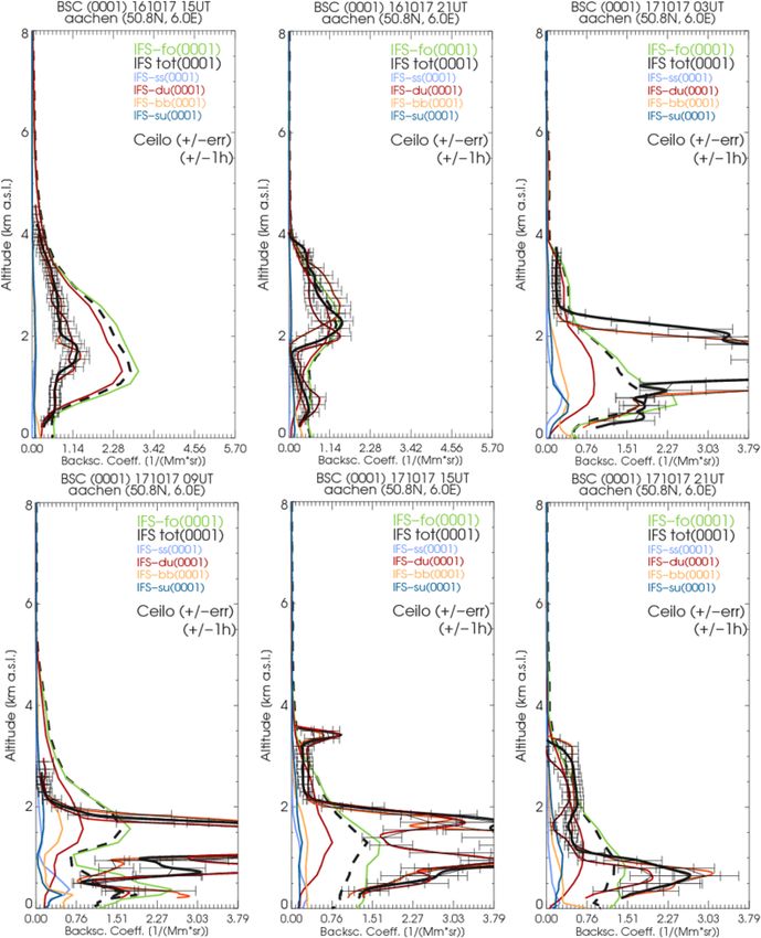
H. Flentje et al.: CAMS aerosol profile evaluation                                                                              1725

                                                                      ±100 m, and no MLH < 400 m a.g.l. can be detected due to
                                                                      artifacts from the overlap correction. Given all these limita-
                                                                      tions, the discussion of MLH is included in this article as it
                                                                      is the most prominent feature in the vertical profile, but it is
                                                                      not intended as a rigorous evaluation.

                                                                      2.4   In situ measurements of particle composition and
                                                                            sizes

                                                                      To interpret the model–observation differences, in situ par-
                                                                      ticle composition measurements are used from the Ger-
                                                                      man GAW global station Hohenpeißenberg (HPB) (47.8◦ N,
                                                                      11.0◦ E; 990 m a.s.l.), (Flentje et al., 2015). The Hohen-
                                                                      peißenberg station is located on a pre-Alpine hill, sticking out
                                                                      300 m above the surrounding forest and/or grassland and rep-
                                                                      resents rural central European conditions. Particle composi-
                                                                      tion observations stem from the quadrupole aerosol chemical
                                                                      speciation monitor (Q-ACSM; Aerodyne Res. Inc., Billerica,
                                                                      MA, USA; Ng et al., 2011) and quartz-/teflon-filter probes
                                                                      analyzed for water-soluble ions with a DIONEX ICS 1000
                                                                      (Henning et al., 2002) as detailed in Flentje et al. (2015).
                                                                      Both measurements’ uncertainties are negligible for global
                                                                      model evaluation. Only the model vertical level of correspon-
                                                                      dence is not unambiguous to determine for mountain stations
                                                                      sticking out from the model orography. The profile evalua-
                                                                      tion circumvents this by excluding stations in steep terrain
                                                                      and through the negligible effect of the orography at higher
                                                                      altitudes. As a compromise for HPB (zobs = 995 m a.s.l.,
Figure 1. Lufft-CHM15k ceilometer network of the Deutscher Wet-       zgeopot-model = 665 m) to capture both surface effects and am-
terdienst (DWD) in 2020, color coded by the number of avail-          bient conditions at an elevated sampling level, we choose
able calibrations per month. Pink dots denote stations without cal-   L54–L60 and L127–L137 for the 60L and the 137L model
ibrated data. Near-real-time QuickLooks and metadata informa-         versions, respectively; see, e.g., Wagner et al. (2015). The
tion are available via http://www.dwd.de/ceilomap/ (last access:      range of concentrations within these altitudes indicates the
25 March 2021).
                                                                      uncertainty.

                                                                      2.5   Concept of evaluation
coded in the gradient (but possibly of different orders) of
the backscatter profile (Teschke and Pönitz, 2010) and its            Given the complexity of spatiotemporal variations of 14 in-
temporal development. The CHM15k firmware calculates up               teracting aerosol types in the IFS-AER model, it is important
to three layers with quality flags from the range-corrected           to reduce the evaluation to a meaningful subset of metrics and
signal (P (z)z2 ) by means of a wavelet transform algorithm           scores and adapt it to the information content of the observa-
(Teschke and Pönitz, 2010). Which of these corresponds to             tion data. This study focuses on the vertical aerosol distribu-
the MLH, however, remains a decision according to speci-              tion and the altitude dependence of the model–observation
ficity, temporal continuity and distinctness. In this respect,        differences (bias) from about 0.3 to 6 km above ground. Be-
Haeffelin et al. (2012) find in their analysis of limitations and     low 0.3 km, the incomplete overlap cannot be corrected with
capabilities of existing mixing height retrieval techniques           sufficient accuracy. Above 6 km, ceilometer data suffer in-
“. . . no evidence that the first derivative, wavelet transform,      creasingly from low SNR and cloud artifacts. To avoid per-
and two-dimensional derivative techniques result in different         turbation of our results by truncated profiles extending verti-
skills to detect one or multiple significant aerosol gradients”.      cally over less than 0.6 km or containing clouds and possibly
While MLH reported by CHM15k definitely lacks reliability             falling precipitation streaks, such profiles are excluded (see
even when robust metrics like maximum daily mixing layer              Sect. 4.2). In the vertical, we distinguish between the surface
heights (MMLHs) are chosen, visual inspection of individual           layer (SL) where the sources of most particles are, the ML
cases illustrates why algorithms fail with ubiquitous complex         and the free troposphere (FT), where long-range transport
scenes and simultaneously provides reasonable estimates of            takes place. Model biases may indicate specific deficiencies
MMLH. The uncertainty of visually inferred MLH is about               in the model but may also stem from uncertainties in the ob-

https://doi.org/10.5194/gmd-14-1721-2021                                                Geosci. Model Dev., 14, 1721–1751, 2021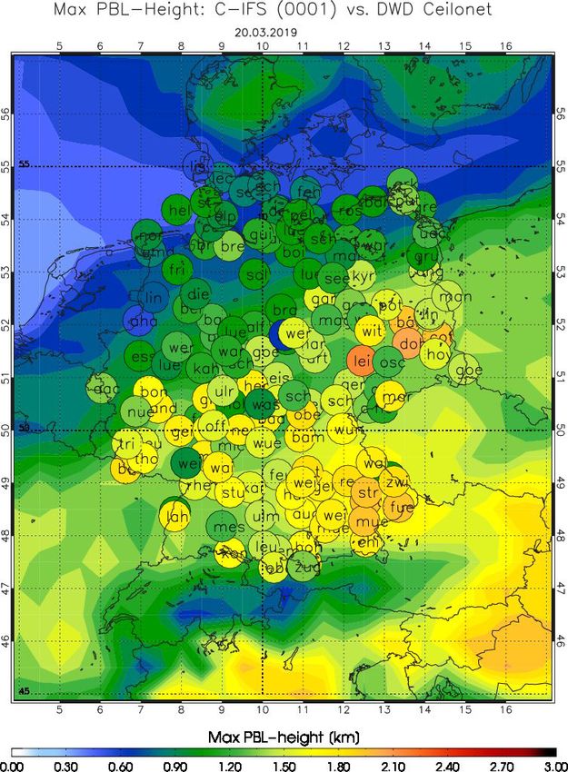
1726                                                                           H. Flentje et al.: CAMS aerosol profile evaluation

servation data or the forward operator or arise from necessary           By considering mean and median values, the skills with
adaptions of the data sets (see Sect. 4.2).                           and without (peaks of) events are distinguished, the latter
   While there are several options to discuss the agreement of        representing more background conditions and less the inter-
forecast and observed backscatter profiles, we use the follow-        annual variability of (mostly dust) events. Negative and pos-
ing metrics and scores: the correlation of model–observation          itive biases are denoted as “low bias” or “high bias”, respec-
profiles evaluates their shape, i.e., efficiency and timeliness       tively; their absolute amount is classified as large or small.
of vertical/horizontal transport, injection heights, represen-        The relative data coverage of 3-hourly profiles from all sta-
tation of the mixing layer and stratification. This is jointly        tions remaining for evaluation is 93 %, 92 %, 89 %, 83 %,
summarized in Taylor diagrams (Taylor, 2001) with the stan-           71 %, 46 % and 16 % at 0.4, 1, 2, 3, 4, 5 and 6 km above
dard deviation coding the variance or amplitude of the pro-           ground, respectively.
files. The bias (as Mm−1 sr−1 ) or modified normalized mean
bias (MNMB) (as a percentage) as a function of time and al-
titude evaluates the sources or sinks (strength) and physical
and chemical transformations, separately for ASM and CTR:             3     Results

                                 N
                             2 X   Masm, ctr (z, ti ) − O(z, ti )     3.1    Bias and MNMB
MNMBasm, ctr (z, t) = 100·     ·                                  ,
                             N i=0 Masm, ctr (z, ti ) + O(z, ti )
                                                                      Figure 2 shows the temporal evolution of bias (upper pan-
where Masm, ctr (z, ti ) and O(z, ti ) denote modeled and ob-         els) and MNMB (lower panels), each for ASM (red/orange)
served values at altitude z and time ti , respectively. Either        and corresponding CTR (green/blue) around vertical model
moving averages over selected altitude ranges (bias time se-          levels spaced by 1 km (0.4, 1, 2, . . .6 km above ground), each
ries) or (e.g., monthly) averages resampled at the model lev-         averaged over ±one model level. The data averaged over
els (bias profiles) are calculated.                                   21 German ceilometer stations become statistically sparse at
   The MNMB is used for comparability within CAMS, be-                higher levels (≥ 6 km). A different perspective, transformed
cause it is better suited to verify aerosol and chemical species      to the whole vertical profiles of monthly mean and median
concentrations compared to verifying standard meteorologi-            bias of β ∗ (z), is shown in Fig. 3 and color coded by each
cal fields. Spatial or temporal variations can be much greater,       month for 2016 to 2019. Actual β ∗ (z) profiles are shown for
and the model biases are frequently much larger in mag-               comparison in Figs. D1 to D4. The following results refer to
nitude. Most importantly, typical concentrations vary quite           Figs. 2 and 3.
widely between different aerosol types, regions and heights,             The bias of β ∗ (z) shows a clearly different behavior near
and a given bias or error value can have a quite different sig-       the surface, in the ML and the FT, with upward tendencies to-
nificance. It is useful therefore to consider bias and error met-     ward the surface, low bulges in the ML, reaching up to ≈ 0.5–
rics that are normalized with respect to observed concentra-          1 km in winter and ≈ 1–2 km in summer, and enhanced vari-
tions and hence can provide a consistent scale regardless of          ation related to irregular long-range transport, mostly of dust,
pollutant type, altitude or region (see, e.g., Elguindi et al.,       in the FT as shown in Fig. 3. Estimated error bars overlay-
2010, or Savage et al., 2013). Moreover, the MNMB is ro-              ing the CTR profiles indicate the significance of the biases.
bust to outliers and converges to the normal bias for biases          The low-bias dips above 6 km are artifacts caused by cloud
approaching zero, while taking into account larger uncer-             boundaries not captured by the quality control. Due to events,
tainties in the observations and the representativeness issue         the mean bias is on average larger and scatters more than the
when comparing coarse-resolved global models versus site-             median, particularly in the FT, which holds little aerosol in
specific station observations.                                        undisturbed situations. Throughout several months, Saharan
   Taylor polar plots combine two statistical measures for            dust events cause a large high bias in the upper ML and the
pairs of profiles, averaged over any optional period of time          FT. A positive impact of the assimilation is reflected by a
(here daily means or medians) and over different stations:            smaller and less variable bias in ASM than in CTR, as shown
the correlation of coincident pairs of modeled and observed           in Fig. 2, where 7 d running means remove the tremendous
vertical profiles plotted along the azimuth, and the standard         variability on daily timescales. Bias and MNMB tend to be
deviation of model profiles normalized to the observation on          lower in CTR (blueish) than in ASM (reddish), particularly
the x axis (Taylor, 2001). This means that correlation is cal-        at lower heights. ASM bias/MNMB show less longer-term
culated over altitude ranges rather than periods of time. The         variation with model changes and seasons and less vertical
ideal agreement or the reference point (observation) is thus          spread. (Note that only ASM is used with cycle 41r1 before
located at the polar coordinate [1, 1]. It is worth noting that       June 2016.) MNMB is less sensitive to absolute β ∗ (z) and
the distance from the reference in Taylor polar plots corre-          thus more clearly shows phases of vertical association and
sponds to the root-mean-square error (RMSE); thus, Tay-               dissociation, and an overall downward trend in 2016–2018
lor plots powerfully display performance changes between              of CTR MNMB turning into an increase in 2019. For ASM,
model versions in a strongly aggregated way.                          this variation is only evident in the FT. With cycle 46r1, bias

Geosci. Model Dev., 14, 1721–1751, 2021                                               https://doi.org/10.5194/gmd-14-1721-2021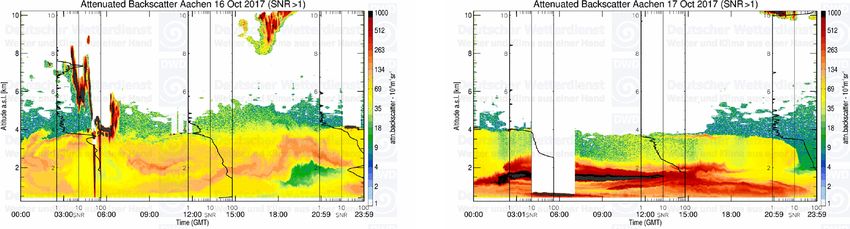
H. Flentje et al.: CAMS aerosol profile evaluation                                                                                      1727

Figure 2. The 7 d running mean bias of β ∗ (z) from ASM (a) and CTR (b) combined from 21 German stations in 2016–2019. Same for
MNMB in panels (c) and (d). Colors refer to different altitudes above ground. Vertical black lines indicate major model updates as in Table 1.

https://doi.org/10.5194/gmd-14-1721-2021                                                     Geosci. Model Dev., 14, 1721–1751, 2021
1728                                                                      H. Flentje et al.: CAMS aerosol profile evaluation

and MNMB in ASM and CTR are vertically closer associ-             til this exceeds the β ∗ (z) threshold above which ceilometer
ated.                                                             data are removed as clouds, such events produce a low bias.
    Over the 4 years, monthly bias profiles have become more      Low biases also occur in the ML (1–2 km lines in Fig. 2)
variable, the means more than medians and CTR more than           during smog periods, e.g., when transport of highly polluted
ASM (Fig. 3). This may reflect changes to model source            air from eastern Europe towards Germany (January 2017,
strengths (see Table 1), larger errors during more frequent       February/March 2018) is not captured by the model (low bias
events and a balancing impact of the assimilation, respec-        of −0.3 Mm−1 sr−1 in February–March 2018; cf. Sect. 3.3).
tively. This scatter is particularly observed in the ML where     At higher altitudes ≥ 5 km, remaining cloud artifacts within
model β ∗ (z) values are on average lower than observed un-       sparse data coverage (low SNR) cause sharp low-bias dips in
til July 2019 and higher thereafter. Particularly CTR shows       Fig. 2.
lower β ∗ (z) bias and MNMB around summers at low heights
(MNMB around −100 %), while ASM remains flatter thanks            3.2   Profile shape – correlation
to the assimilation (Fig. 2). SL biases stick out high (up to
0.3 Mm−1 sr−1 ) with cycle 41r1 T255 in spring 2016 and           The Pearson correlation coefficient (r) of model–observation
with cycle 46r1 after July 2019 (up to 0.4 Mm−1 sr−1 ). In be-    β ∗ (z) profile pairs specifically quantifies the covariance of
tween, they were smaller or negative as shown in Fig. 2 and       vertical variability, i.e., the shape of the profiles, independent
Table 2. A bias increase with cycle 46r1 at 0.4/1 km a.g. cor-    of the bias. The ML and eventual particle plumes in the FT
responds to overestimated NO3 , NH4 and OM in the model,          govern this correlation. Again, elimination of clouds and the
as discussed with respect to GAW surface data in Sect. 3.3.       overlap range is essential. Apart from large event-driven sit-
    Though seasonal regularities are disturbed by five irreg-     uational variability, the profile correlation exhibits no long-
ular model updates in the 2016–2019 period, bias/MNMB             term tendency but displays a clear seasonal cycle with better
in ASM show opposing seasonal cycles in the lower                 agreement in winter and less in summer, as shown in Fig. 5.
(0.4 km a.g.) and the upper (2 km a.g.) ML with ampli-            Overlain in Fig. 5 are vertical lines indicating seasonally ir-
tudes of 0.2 Mm−1 sr−1 /40 % (summer maximum) and                 regular model upgrades and mean values over the IFS cy-
0.1 Mm−1 sr−1 /70 % (summer minimum), respectively                cle periods from Table 1. The mean correlations within the
(Fig. 4). Figure 2 shows this particularly before cycle 43r3 in   IFS configuration periods do not vary significantly (cf. Ta-
October 2017. The seasonal amplitude is small at the inter-       ble 2), and their differences reflect the seasonal cycle rather
mediate level 1 km a.g. The summer minimum is evident up          than indicating changes of the model performance. Individ-
to 3 km (MNMB even to 4 km a.g.), while it is variable due to     ual (3-hourly) profile pairs or longer temporal averages have
Saharan dust events at 5 and 6 km a.g. A weekly cycle is not      been considered, whereby the former penalizes already small
significant in the bias nor the MNMB, indicating a negligible     time shifts or displacements (and yields lower r). Diurnal or
influence of short-term anthropogenic emissions which             longer averages reduce influence from early/lagged transport
are not captured by the inventories’ temporal resolution (1       as well as the dominant diurnal cycle of the ML and are more
month).                                                           sensitive to irregular events. On a monthly basis, also me-
    Periods with opposing high bias in SL or ML and low           dian profiles are considered to evaluate specifically the model
bias in FT indicate vertical displacement of aerosol within       background profile (Appendix D, Figs. D1–D4).
the profile. While expected within individual profiles, it of-       Generally, increasing correlation is found between IFS-
ten also lasts for longer periods, as shown in Fig. 2, e.g.,      AER fields and individual station profiles, with longer aver-
in April–June 2016 and repeatedly until cycle 45r1 in mid-        aging times: while only 50 %–60 % of the observed 3-hourly
2018, whereupon it largely disappears. Longer periods are         vertical variability is explained by IFS-AER (r3hly = 0.5–
evident as oscillations even in the monthly mean profiles         0.6), the explained fraction increases to 70 %–80 % for di-
in Fig. 3. The effect is more distinct for ASM and may be         urnal average profiles (r1dly = 0.7–0.8) as shown in Fig. 5.
attributed to adaptions by the assimilation of AOD which          Thus, spatiotemporal aggregation defines the information
adds no direct height information. Spatiotemporal shifts be-      to be revealed. Aerosol changes are very often not timely
tween the model and observations result in low-bias or high-      and/or (vertically) displaced on a timescale of a few hours,
bias oscillations with time and mostly cancel out within a        but longer (or more extended) events and developments are
day. The corresponding fractional skill score is discussed        quite reliably captured by IFS-AER. This is particularly true
in Sect. 3.4.2. Outstanding high-biased monthly profiles          for Saharan dust transport where nearly all events are re-
(Figs. 3 and 2) or high-bias peaks are mostly related to Sa-      produced but the large concentrations (large β ∗ (z)) com-
haran dust events, e.g., in April and June 2016, June, July       bined with small-scale inhomogeneity give rise to larger un-
and October 2017, January and April 2018 and June–July            certainties as well (see Sect. 3.4.1). The middle panel of
and October–December 2019 (see Sect. 3.4.1). However, oc-         Fig. 5 shows the variance and provides numbers of daily
casionally, SD particles induce cloud formation (e.g., 16–17      average vertical profiles normalized to that of the observa-
October 2017) which largely increases the β ∗ (z) signal in       tions as normalized standard deviation (NSD). The time se-
spite of the constant dust aerosol load (see Appendix B). Un-     ries and Table 3 reveals marked differences between the IFS

Geosci. Model Dev., 14, 1721–1751, 2021                                            https://doi.org/10.5194/gmd-14-1721-2021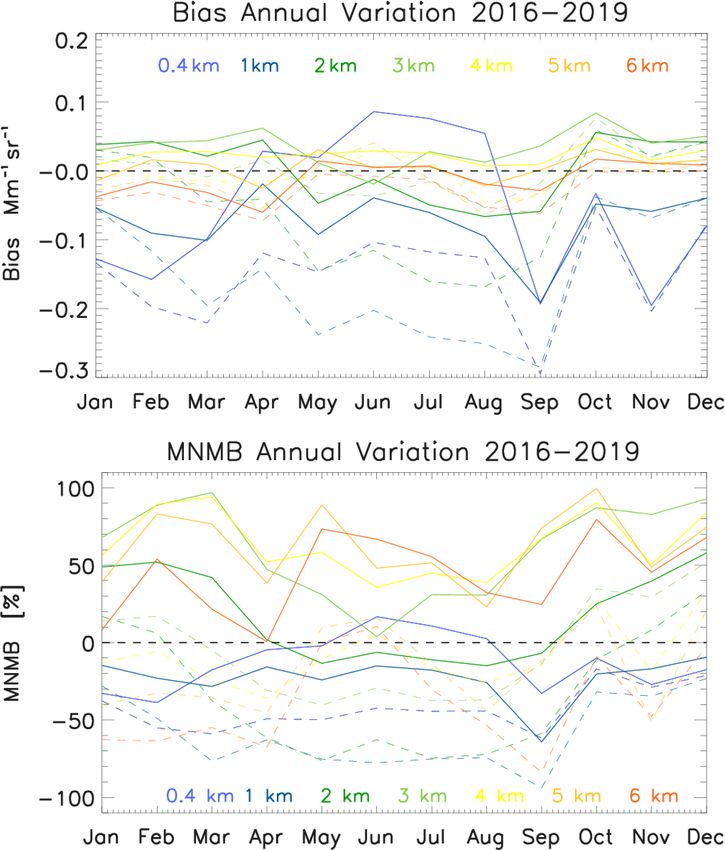
H. Flentje et al.: CAMS aerosol profile evaluation                                                                              1729

Figure 3. Monthly mean (left pair) and median (right pair) profiles of bias ASM/ceilometer (left) and CTR/ceilometer (right), combined
from 21 German stations in 2016–2019. At higher altitudes, the profiles are partly contaminated by remaining cloud artifacts.

https://doi.org/10.5194/gmd-14-1721-2021                                                Geosci. Model Dev., 14, 1721–1751, 2021

1730                                                                           H. Flentje et al.: CAMS aerosol profile evaluation

Table 2. Bias [Mm−1 sr−1 ] and MNMB [%] of β ∗ (z) for ASM and CTR runs at 0.4, 1 and 4 km altitude above-ground averages within the
different model configurations of Table 1.

                                          41r1 (T255)   41r1 (T511)        43r1      43r3        45r1      46r1
                         ASM bias
                         0.4 km                 0.04          −0.04       −0.07     −0.04      −0.11        0.2
                         1 km                  −0.01          −0.08       −0.11     −0.01      −0.12       0.02
                         4 km                   0.03           0.03        0.03      0.02        0.0       0.06
                         CTR bias
                         0.4 km                     –         −0.16       −0.21     −0.07     −0.21       0.09
                         1 km                       –         −0.17       −0.22     −0.03     −0.23      −0.06
                         4 km                       –          0.01       −0.02     −0.01    −0−03        0.07
                         ASM MNMB
                         0.4 km                    5             −10        −20        −8        −23         34
                         1 km                     −6             −15        −30        −4        −33          1
                         4 km                     86              82         67        65         29         99
                         CTR MNMB
                         0.4 km                     –            −47        −68      −20         −54         16
                         1 km                       –            −57        −82      −18         −78        -20
                         4 km                       –             34         −2       −6         −67         63

                                                                       cycles, given for ASM/CTR, separately: profile variance ap-
                                                                       proaches the observations (NSD = 0.97/0.93) during cycle
                                                                       41r1 before June 2016 and NSD = 0.95/0.96 during cycle
                                                                       46r1. Only about half the observed variance is simulated
                                                                       during cycles 41r1 after July 2016 (NSD = 0.52/0.50), 43r1
                                                                       (NSD = 0.46/0.45) and 45r1 (NSD = 0.51/0.52). Interme-
                                                                       diate values (NSD = 0.67/0.78) are found during cycle 43r3.
                                                                       A similar measure like NSD (analog to AOD bias) is the
                                                                       vertically integrated β ∗ (z) bias. It is dominated by the ML
                                                                       and/or events as in Fig. 2 but has the limitation that every
                                                                       single profile has weather-dependent vertical extension. No
                                                                       clear ruptures as for NSD appear at the model upgrade times
                                                                       for the integrated β ∗ (z) diurnal profile bias in Fig. 5c. It is not
                                                                       clear whether this can be interpreted in terms of model up-
                                                                       grades where several adaptions of sources took place. For ex-
                                                                       ample, sea salt as a large contributor to high β ∗ (z) bias in the
                                                                       ML (Chan et al., 2018) was reduced inland after June 2018
                                                                       by redistributing mass from fine to coarse particles (Rémy
                                                                       et al., 2019). As of July 2019, NO3 and NH4 were added
                                                                       and probably too much, as discussed in Sect. 3.3. On the
                                                                       other hand, the substantial increase of the OM load in Febru-
                                                                       ary 2017, clearly evident at the surface (Sect. 3.3) seemingly
                                                                       did not affect the profile integral.
                                                                          A more condensed way than Fig. 5 to descriptively visu-
                                                                       alize performance changes between model versions is Taylor
Figure 4. Annual variation of bias and MNMB of β ∗ (z) for ASM
                                                                       polar plots, as displayed in Fig. 6 and explained in Sect. 2.5.
and CTR (dashed) combined from 21 German stations in 2016–
                                                                       Here, the average performance during the six IFS-AER con-
2019.
                                                                       figurations in Table 1 are summarized in terms of correla-
                                                                       tion, normalized standard deviation and the plotting distance

Geosci. Model Dev., 14, 1721–1751, 2021                                                  https://doi.org/10.5194/gmd-14-1721-2021
H. Flentje et al.: CAMS aerosol profile evaluation 1731
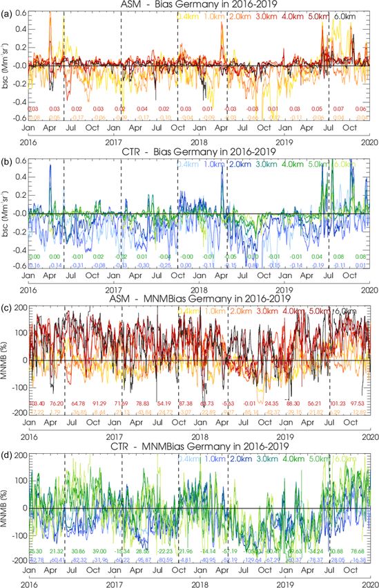
Figure 5. Pearson’s correlation coefficients (r; a), standard deviation normalized towards ceilometer observations (b) and integrated bias of
daily average β ∗ (z) profiles of IFS-AER versus ceilometers for 2016–2019. Red crosses denote ASM; blue crosses denote the control run.
The 3 d moving average line and median values over the periods with constant model configurations are added.
towards the reference, i.e., the root mean square error (Tay- 3.3 Particle composition and size at surface level
lor, 2001). Accordingly, the model system has not system-
atically evolved towards improved representation of the pro-
To better understand the differences between modeled
file shape, though mean values around r1dly = 0.7 are already
and observed backscatter β ∗ (z) profiles, near-surface
quite good. However, after some changes, finally the over-
mass concentrations MC of the prognostic aerosols in
all variance of the profile became nearly realistic on aver-
IFS-AER, namely PM10 , sulfate (SO4 ), nitrate (NO3 ),
age after the implementation of NO3 and NH4 and adaptions
ammonium (NH4 ), BC and OM as well as qualitative
to SO4 , organics and dust in cycle 46r1 in July 2019. The
proxies for sea salt (SS) and mineral dust (MD) are
differences between ASM and CTR are small. It should be
compared to surface in situ observations. All particle
noted that individual covariances of modeled and observed
concentrations are modeled and measured (in situ) in dry
profiles vary quite strongly with time and location/station,
state without hygroscopic water uptake. PM10 is calcu-
meaning that many situations cannot be closely captured and
lated from the model mass mixing ratio (mmr) according
even the observations may partly not be representative due
to the formula used in IFS-AER (Rémy et al., 2019):
to undetected artifacts (clouds, overlap correction, misalign-
PM10 = ρ([SS1 ]/4.3 + [SS2 ]/4.3 + [MD1 ] + [MD2 ] +
ment, etc., not removed by the quality control).
0.4[MD3 ] + [OM] + [BC] + [SO4 ] + [NO31 ] + [NO32 ] +
[NH4 ]), whereby [Xi ] denotes the mmr of the ith size bin
of the size-resolved species and ρ is the density of air. The
“dust” variable is not directly measured but approximated by
https://doi.org/10.5194/gmd-14-1721-2021 Geosci. Model Dev., 14, 1721–1751, 20211732 H. Flentje et al.: CAMS aerosol profile evaluation
Figure 6. Taylor plot combining Pearson’s correlation coefficients (azimuth) and standard deviation normalized towards ceilometer obser-
vations (radius) from daily average β ∗ (z) profiles of IFS-AER versus ceilometers for 2016–2019. (a) Median of all data; (b) mean over 221
Saharan dust days as defined in Sect. 3.4.1. Red dots denote ASM; blue dots denote the corresponding CTR. Note the different x and y axes.
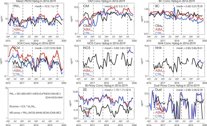
MD = PM10 −[OM]−[BC]−[NO3 ]−[NH4 ]−[SO4 ]−[Cl] Total suspended sea salt is equally overestimated in ASM
and inferred on event basis to discuss contingency of events and CTR with mean MC around 1.8 µg/m3 , while the esti-
in Sect. 3.4.1. Mineral dust sizes at HPB are mostly smaller mated abundance at the far inland HPB site is only 0.02–
than 10 µm and its composition is largely disjunct from the 0.3 µg/m3 , however with large error bars of ±0.3 µg/m3 due
other IFS-AER particle types. Chlorine (Cl) is used as a to the hard-to-sample coarse mode (5–20 µm) which con-
proxy for NaCl in sea salt, stoichiometrically corrected for tributes about 0.3 µg/m3 to the SS concentration in the model.
the sodium Na portion (mNa /mCl ≈ 22/35) and for ≈ 7 % The seasonal variation by roughly an order of magnitude
of additional minor components like SO4 , Mg, Ca, etc. A seems realistic. The large uncertainties and increases of bias
rigorous evaluation of composition-resolved MC is beyond in the PBL associated with SS has already been discussed
the scope of this article, but a sanity check with data from in Chan et al. (2018). To this end, the above-mentioned ap-
the GAW global station (HPB) provides insight into the proximation of SS via Cl has a negligible impact. The ob-
representation of individual aerosol types. served dust proxy contributes only 4 %–6 % to the annual
As shown in Fig. 7, the dry surface mass concentra- average mass at HPB (Flentje et al., 2015). The seasonal-
tion PM10 for ASM (10.3 µg/m3 ) and CTR (7.9 µg/m3 ) ity is reproduced, but mean summer contributions around
roughly corresponds to HPB data (7.9 µg/m3 ). The assimila- 10 µg/m3 would require much more events than observed and
tion seems to bias surface concentrations a bit high. Species simulated, which confirms that dust concentrations are over-
are detailed in Table 3. PM10 approaches HPB data after the estimated not only near the surface but also in the higher ML
increase of OM with cycle 43r1 (February 2017), though this and the FT, as noted in Sect. 3.1. The assimilation correc-
was partly compensated by a parallel decrease of SO4 ; it tion to dust MC of few µg/m3 is too small. These results are
is, however, overestimated as of cycle 46r1 after July 2019 not affected by mass-to-backscatter conversion nor humidity
due to the introduction of NO3 and NH4 , which are sim- and, due to averaging over the lowest 300 m a.g., are not sen-
ulated roughly 3 µg/m3 (∼ 300 %) and 0.3 µg/m3 (∼ 60 %) sitive to the model level selected to represent surface concen-
too high at HPB, respectively. Further changes with cycle trations at HPB. The regional representativeness is limited to
43r3 (October 2017) synchronize the phase but exaggerate rural central Europe (Putaud et al., 2010) where compara-
the amplitude of the SO4 annual cycle which together with tively small concentrations prevail, as discussed in Sect. 4.
the dominating high-biased contribution from OM causes
most of the PM10 overestimation near the surface in sum- 3.4 Long-range transport
mers since 2018. After sulfate was reduced in cycle 43r3
and beyond (Rémy et al., 2019), SO4 in CTR agrees remark- The DWD ceilometer network follows the 3-D dispersion of
ably well with HPB, while summer concentrations are by 2– optically efficient particles like dust or smoke and is therefore
4 µg/m3 too high in ASM. BC, which contributes only about particularly suitable to verify the timeliness of long-range
5 % in mass, has evolved quite realistically with a slightly aerosol transport in IFS-AER in a qualitative way. Against
more decreasing trend in 2016–2019 than observed. Proba- this, automated rendering of 2-D time–height sections from
bly, emission inventories overestimate the decreasing trend the ensemble of stations to evolving 3-D fields is a challenge
over Europe where the decline has leveled off in the last beyond the scope of this article, and advanced metrics like
decade. fractions skill score (Roberts, 2008) still have to be adapted.
Simpler options are to compare time–height slices at fixed
Geosci. Model Dev., 14, 1721–1751, 2021 https://doi.org/10.5194/gmd-14-1721-2021H. Flentje et al.: CAMS aerosol profile evaluation 1733
Table 3. Concentrations [µg/m3 ] of IFS-AER prognostic aerosols by ASM and CTR versus GAW in situ measurements at the Hohenpeißen-
berg station, averaged over constant model configuration periods as defined in Table 1.
41r1 (T255) 41r1 (T511) 43r1 43r3 45r1 46r1
ASM PM10 11.61 6.91 9.40 11.30 10.71 13.76
CTR PM10 10.43 5.55 6.37 10.06 6.92 11.36
GAW PM10 7.74 8.33 7.90 8.20 8.37 5.81
ASM OM 1.01 1.50 4.08 5.93 6.06 4.74
CTR OM 0.94 0.90 2.18 4.17 3.46 2.87
GAW OM 2.52 2.63 2.71 2.63 3.10 1.79
ASM BC 0.54 0.61 0.56 0.33 0.30 0.18
CTR BC 0.50 0.49 0.20 0.36 0.15 0.11
GAW BC 0.35 0.47 0.35 0.46 0.39 0.30
ASM SO4 5.60 3.02 1.80 1.03 1.97 1.04
CTR SO4 4.60 1.46 0.70 0.78 0.78 0.40
GAW SO4 0.81 0.72 0.82 0.86 1.00 0.51
ASM NO3 – – – – 3.21 3.95
CTR NO3 – – – – 3.63 3.85
GAW NO3 0.70 1.22 0.95 1.67 1.53 0.81
ASM NH4 – – – – 0.72 0.88
CTR NH4 – – – – 0.80 0.87
GAW NH4 0.47 0.62 0.60 0.92 0.89 0.45
ASM SS 2.38 1.35 2.14 2.52 1.22 1.24
CTR SS 2.25 1.32 2.16 2.60 1.13 1.20
GAW SS 0.17 0.13 0.14 0.19 0.14 0.13
ASM DU 4.34 1.41 2.42 2.82 2.44 6.04
CTR DU 4.31 2.48 2.90 3.90 2.71 6.84
GAW DU 1.94 2.78 2.28 1.58 2.69 1.79
locations (stations), analyze representative cases or evaluate these threshold yield “excess” and “miss” rates near zero,
the representation of events qualitatively. In aged air masses 221 “hit” days and 271 zeroes. Hits (zeroes) are SDDs (clear
far from the sources, chemical transformations slow down days) identified in both data sets; “excess” SDDs are simu-
and transport of particle layers/plumes becomes more pas- lated but not observed and “misses” denote observed SDDs
sive. This reflects in wide consistency of aerosol fields in the that are not reproduced by IFS-AER. Due to the uncertain
IFS model with large-scale dynamical structures in the mid- identification of faint aerosol layers based on ceilometers
dle and upper troposphere (e.g., Flentje et al., 2005). and trajectories, the majority (two-thirds) of days in between
these thresholds remain unclassified. This is, however, no se-
3.4.1 Mineral dust vere limitation to this analysis, which is meant to confirm
qualitatively the high reliability of the forecasts with respect
The previous sections showed that Saharan dust loads over to decided SDDs and non-SDDs.
Germany are overestimated at the surface and throughout As several improvements were made to emission, size dis-
the profile. The realistic seasonality (Fig. 7) and the rea- tribution and (wet) deposition of dust (Rémy et al., 2019), a
sonable correlation (Fig. 5) however suggest that time and Taylor diagram for the subset of SDDs with modeled maxi-
also vertical position of SD plumes are mostly captured mum AOD550 nm,dust > 0.03 in Fig. 6 shows the development
in IFS-AER, as long as the scales are sufficiently large. It of dust simulation by IFS-AER during the 2016–2019 pe-
can further be shown that IFS-AER forecasts have a high riod. On SDDs, the correlation of profiles (shapes) is lower
score in capturing or reliably excluding significant Saha- (r = 0.4–0.6 instead of r = 0.6–0.8), while standard devia-
ran dust days (SDDs), which are inferred from the observa- tion (coding the amplitude of β ∗ (z)) is higher. The first in-
tions by visual inspection of 2-D network composite plots dicates spatiotemporal or vertical shifts of layers/plumes, the
and backward trajectories and from the model by choos- latter reflects overestimation of dust concentrations but is not
ing a reasonable threshold for maximum dust AOD within directly scaled to the SD bias due to the large influence of
a box of 1◦ × 1◦ around selected ceilometer stations. Defin- the ML on the profile. These findings confirm the analysis
ing days with maximum AOD550 nm,dust > 0.03 (maximum by Rémy et al. (2019) who state a good capability to repro-
AOD550 nm,dust < 0.001) as SDDs (non-SDDs) in the model duce dust events as detected by Aerosol Robotic Network
and within the inherent uncertainties of type identification, (AERONET) station data (Holben et al., 2001). According
https://doi.org/10.5194/gmd-14-1721-2021 Geosci. Model Dev., 14, 1721–1751, 20211734 H. Flentje et al.: CAMS aerosol profile evaluation
Figure 7. Comparison of mass concentrations averaged over IFS levels L54–L60/L127–L137 for L60/L137 model versions and measured
by ACSM and filter probes at the Hohenpeißenberg GAW station for 2016–2019. From the top left to the bottom right: PM10 , OM, BC, SO4 ,
NO3 and NH4 , chlorine, sea-salt and dust proxies as described in the text. Vertical black lines indicate major model updates as in Table 1.
Note the different y ranges!
to the different trajectories, the long-range transport pathway randomly displaced or missed because the information con-
(via the Atlantic, Mediterranean, etc.) does not effect the ac- tent of the model fields does not match the resolution of
curacy of timing/positioning of plumes, while the scale re- the observations, which the other way round, are not rep-
duction during regional stirring and dispersion is the main resentative for the model grid box. For profile correlation,
reason degrading the representation of the vertical profile the usefulness threshold of scales is for IFS-AER presently
shape. of the order of 0.5 d and 100 km. An approach towards FSS
would be to draw polygons either outlining the boundary of
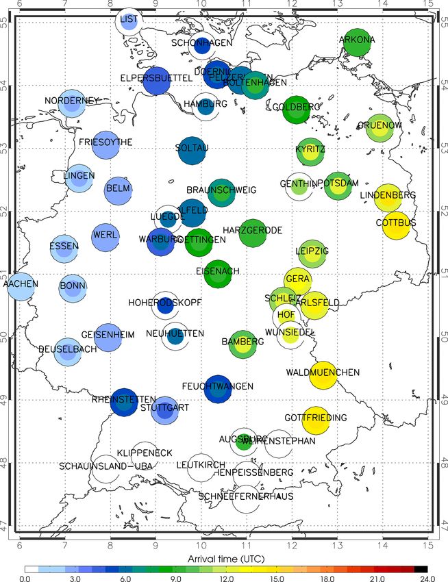
3.4.2 Fractions skill score an individual SD plume observed at a given time at differ-
ent ceilometer stations or, alternatively, refer to the overlap
The penalizing of slightly vertically displaced aerosol lay- of plumes in time–height sections at individual stations. An-
ers yielding a low or even anti-correlation in Sect. 3.2 hints other metric to quantify the model performance for coherent
to the fact that a useful assessment of the positioning (in plumes in a quasi-stationary flow is the relative deviation of
space and time) of an aerosol plume requires not only a ref- arrival/departure times of plumes/layers at station positions
erence to point locations but also to their vicinity. Such a in model and observation as visualized in Fig. 8 for the SD
skill score shall distinguish nearly correct positioned features plume on 16 October 2017. Composite bullets with color-
from deviations by a bigger margin. An approach to quan- coded arrival times observed in 2-D β ∗ (z) ceilometer sec-
tify the degree of overlap of simulated and observed aerosol tions (outer ring) and corresponding model fields (inner bul-
structures is the fractions skill score (FSS; Roberts, 2008; let) illustrate the slightly delayed arrival (0–1 h) of the model
Skok and Roberts, 2016). The perceived accuracy increases plume in western Germany, its catchup in the middle and
with larger scales, longer averaging, elimination of outliers, again lagged arrival (0–2 h) in the eastern part. The uncer-
etc. Thus, reasonable scales must be analyzed to balance the tainty of determination is about 1 h. This plume was neither
processes of interest and the useful level of detail to be no- observed nor simulated in the very south of Germany.
tified. For example, small (subgrid)-scale structures appear
Geosci. Model Dev., 14, 1721–1751, 2021 https://doi.org/10.5194/gmd-14-1721-2021You can also read