Evaluation of Satellite Precipitation Products in Simulating Streamflow in a Humid Tropical Catchment of India Using a Semi-Distributed ...
←
→
Page content transcription
If your browser does not render page correctly, please read the page content below
Article

Evaluation of Satellite Precipitation Products in
Simulating Streamflow in a Humid Tropical
Catchment of India Using a Semi-Distributed
Hydrological Model
Thalli Mani Sharannya 1,*, Nadhir Al-Ansari 2, Surajit Deb Barma 1 and Amai Mahesha 1
 1 Department of Water Resources and Ocean Engineering, National Institute of Technology Karnataka,
   Mangalore 575025, India; surajitdb@gmail.com (S.D.B.); amaimahesha@gmail.com (A.M.)
 2 Department of Civil, Environmental and Natural Resources Engineering, Lulea University of Technology,

   971 87 Lulea, Sweden; nadhir.alansari@ltu.se
 * Correspondence: sharannyatm@gmail.com

 Received: 30 July 2020; Accepted: 22 August 2020; Published: 26 August 2020

 Abstract: Precipitation obtained from rain gauges is an essential input for hydrological modelling.
 It is often sparse in highly topographically varying terrain, exhibiting a certain amount of
 uncertainty in hydrological modelling. Hence, satellite rainfall estimates have been used as an
 alternative or as a supplement to station observations. In this study, an attempt was made to
 evaluate the Tropical Rainfall Measuring Mission (TRMM) and Climate Hazards Group InfraRed
 Precipitation with Station data (CHIRPS), employing a semi-distributed hydrological model, i.e.,
 Soil and Water Assessment Tool (SWAT), for simulating streamflow and validating them against
 the flows generated by the India Meteorological Department (IMD) rainfall dataset in the Gurupura
 river catchment of India. Distinct testing scenarios for simulating streamflow were made to check
 the suitability of these satellite precipitation data. The TRMM was able to better estimate rainfall
 than CHIRPS after performing categorical and continuous statistical results with respect to IMD
 rainfall data. While comparing the performance of model simulations, the IMD rainfall-driven
 streamflow emerged as the best followed by the TRMM, CHIRPS-0.05, and CHIRPS-0.25. The
 coefficient of determination (R2), Nash–Sutcliffe efficiency (NSE), and percent bias (PBIAS) were in
 the range 0.63 to 0.86, 0.62 to 0.86, and −14.98 to 0.87, respectively. Further, an attempt was made to
 examine the spatial distribution of key hydrological signature, i.e., flow duration curve (FDC) in the
 30–95 percentile range of non-exceedance probability. It was observed that TRMM underestimated
 the flow for agricultural water availability corresponding to 30 percent, even though it showed a
 good performance compared to the other satellite rainfall-driven model outputs.

 Keywords: CHIRPS; FDC; hydrological signature; SWAT; TRMM; Western Ghats

1. Introduction
      Precipitation is a critical element of the hydrological cycle which is responsible for replenishing
freshwater on the planet. It is an essential input for hydrological modelling and also forms the basis
of hydrological, agricultural research applications, environment studies, and climate change studies
[1,2]. It is seen that areas of high rain gauge density give more reliable precipitation estimates than
those of low-density areas [3,4]. However, due to economic constraints and infeasible natural
conditions, such as in the Arctic [5] and in the Tibetan Plateau, ground-based observations are usually
sparse, especially in several developing countries, where ground-based rainfall observation networks

Water 2020, 12, 2400; doi:10.3390/w12092400                                    www.mdpi.com/journal/water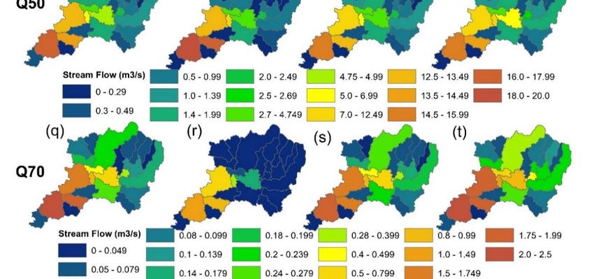
Water 2020, 12, 2400                                                                               2 of 25

have always been relatively sparse [6–8]. Hence, precipitation data retrieved from satellite sensors
act as a valuable source for several research applications [9,10]. Recently, many satellite rainfall
estimates were made available free of cost from different sources with high temporal and spatial
resolutions providing global coverage at sub-daily, daily, and monthly time steps [11]. Various
rainfall satellite products are available worldwide which could be broadly categorised into satellite
only (SM2-RAIN product), satellite-adjusted (PERSIANN CDR, GPCC), reanalysis category (CHIRP,
ERA, and MSWEP), and near real-time products (TRMM RT) [12–14]. With the advancement in
blending infrared, microwave, and gauge datasets and availability of spatial and global coverages,
multi-temporal resolutions have increased the applicability of satellite rainfall datasets over a wide
range of applications. However, signal calibration and corrections for beam filling, bright band, and
attenuation could be considered as their limitations [15,16]. These satellite data could be validated
either by comparing them to station data and ground-based radar estimates or by confirming their
predictive ability and effectiveness through a hydrological modelling framework [17].
      A comparative analysis of various satellite-derived datasets with gauge datasets is available
elsewhere [18–21]. The statistical evaluation displays the inherent data consistency of the satellite
precipitation data. In contrast, the hydrological simulation of these data gives insight into the utility
of the datasets within the given application. Many investigators addressed the assessment and
evaluation of satellite precipitation products’ efficiency for statistical and hydrological analysis
[13,17,19,22], out of which only a few were conducted over the Indian basins [23,24]. Several
investigations [19,25,26] have reported that better statistical analysis for precipitation data has not
yielded reliable hydrological analysis. This mandates the testing of all precipitation data using
hydrological models for different applications.
      Flow duration curve (FDC) performance assessment can help assess the ability of the
hydrological model to simulate streamflow [27]. The FDC is perceived as a legitimate descriptor for
catchments. The FDC is described by [28] as ‘a key runoff variability signature’ that could be applied
for obtaining the catchment response as daily streamflow magnitude and as a function of the percent
of time exceeded [29]. The use of FDC provides more information on the hydrological activity of the
modelled basins, as well as their underlying processes [30,31]. The hydrological models have the
advantage of simulating continuous runoff but come at the expense of calibrating them with a specific
objective function like NSE. Such models are also biased towards high and medium flows and
underperform over regression techniques when they come to low flow and dynamic flows [32].
Hence, the present study is focused on characterising the medium and high flows. To the best of the
authors’ knowledge, spatial representation of these flow duration curves for evaluating the ability of
satellite-based precipitation data has not been explored earlier for a poorly gauged catchment. The
main objective of this paper is to derive the streamflow from different sets of precipitation data and
their spatiotemporal variability. An attempt is made here to examine the spatial distribution of FDC
in the range Q5–Q70, i.e., 95–30 percentile range of non-exceedance probability. Since the study
catchment experiences high flow from June to November due to the Indian monsoon season (June to
September), and low flows over the rest of the year, it is of interest to study streamflow over the range
of the 30 to 90 percentile range.
      Based on the literature above, there exists a need to examine the effectiveness and reliability of
precipitation data for hydrological simulations. Because of the above considerations, the present
work is framed with the following objectives: (i) to evaluate the capability of satellite-based
precipitation data for simulating the streamflow using a semi-distributed hydrological model
(SWAT); (ii) to evaluate the responsiveness of calibrated parameters under different scenarios for
simulating the streamflow with gauge-based and satellite precipitation datasets; (iii) to quantify the
uncertainty in the parameters for hydrological process simulation; (iv) to represent the key
hydrological signatures using the flow simulated from different datasets with optimised parameters
for a typical Western Ghat catchment of India. The novelty of this paper lies in utilising the ability of
the SWAT model to generate the streamflow for ungauged subcatchments by gauge and satellite
precipitation datasets and using them to derive hydrological signatures spatially. The simulation of
the flow from different satellite datasets under different calibration scenarios is yet to be explored for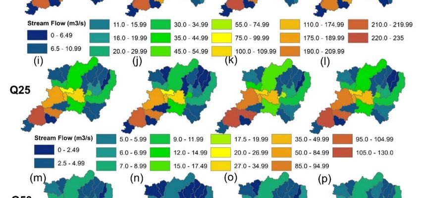
Water 2020, 12, 2400                                                                              3 of 25

the Western Ghat catchments of India. This is the first study to use satellite precipitation products for
generating hydrological signatures. A similar approach using calibration scenarios for developing
hydrological signatures in ungauged catchments could be carried out to formulate a hypothesis
regarding the effects of sensitive parameters of each dataset to understand the catchment
characteristics worldwide. The above investigations would help to identify the most appropriate
dataset for hydrological application.

2. Materials and Methods

2.1. Study Area
     The Western Ghats (WG) are the mountain ranges along the west coast of India that extend for
about 2300 km parallel to the seacoast. They are located at a distance of about 100 to 200 km from the
seacoast across the Gujarat, Maharashtra, Karnataka, and Kerala states of India [33]. The Gurupura
river is one of the west-flowing rivers originating in the WG of India, at an elevation of 1880m above
mean sea level. The catchment has two river gauging stations at Addoor and Polali, which are
maintained by the Central Water Commission, Government of India and the Public Works
Department of the Government of Karnataka [34], respectively. For the present investigation, the
Addoor gauging station was selected, which drains out an area of about 840 km2 (Figure 1). The west
coast consists of a coastal plain with agricultural cropland followed by the lateritic plateau
dominating the central portion of the river basin and dense forest in the hilly regions of the Western
Ghats. The mean annual precipitation over the basin is about 3812 mm, mostly occurring during the
southwest monsoon season (June to September). It is characterised by a humid and tropical climate
with a temperature range of 20 to 35 °C. It is one of the vital river basins within the WG, which
supplies drinking water to the suburban region of Mangalore city and a few industrial units and
agricultural activities in the basin.

                           Figure 1. Location map of the Gurupura river basin.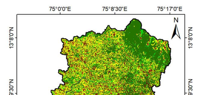
Water 2020, 12, 2400                                                                            4 of 25

2.2. Hydrological Model
      The Soil and Water Assessment Tool (SWAT) is a physically based semi-distributed model
intended to compute and route water, sediments, and contaminants from the individual drainage
units (subbasins) to their outlets throughout the river basin [35]. The SWAT model is widely used for
simulating biophysical processes, viz., erosion, vegetative growth, water quality, streamflow, and
pollutant concentration for quite a long period [36–38]. It segments the river basin into several
subbasins leading to Hydrological Response Units (HRUs), defined by various combinations of land
use, soil characteristics, topography, and management systems.
      The hydrological cycle is determined based on water balance, which is regulated by climate
inputs such as daily precipitation and maximum/minimum air temperature. The SWAT simulates
the daily, monthly, and annual water fluxes and solutes in river basins using daily input time series.
The simulations begin by calculating the amount of water, sediment, and pollutants loading to the
main channel from the land of each subbasin; loads are conveyed and routed through the streams
and reservoirs within the basin. The Shuttle Radar Topography Mission (SRTM), the Digital Elevation
Model (DEM) (Figure 1), the Land use land cover map (LULC) obtained from the supervised
classification technique (maximum likelihood algorithm) for the year 2003 (Figure 2), and the soil
map were the input to the SWAT model. The spatial/temporal resolution and source of data obtained
are listed in Table 1. After providing the land use and soil maps as input, a total of 27 subbasins and
266 Hydrological Response Units (HRU) were generated. The residual climate data such as solar
radiation, relative humidity, and wind speed could be supplied or generated by the user-defined
weather generator (Table 1).

                               Figure 2. LULC used for the SWAT model.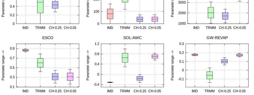
Water 2020, 12, 2400                                                                                                                              5 of 25

                                                         Table 1. Data source and description.

                                                       Spatial/Temporal
                        Input Data Type                                                                       Source/Period
                                                          Resolution
        SRTM Digital Elevation Model (DEM)                   30 m/-                                https://earthexplorer.usgs.gov/
                    Land use map                             30 m/-                     Landsat imageries (http://earth explorer.usgs.gov/2003)
                       Soil map                             500 m/-               Food and Agriculture Organization of the United Nation (FAO)/2002
       Meteorological data (rainfall and min-max
                                                           0.25°/daily                      India Meteorological Department (IMD)/1998–2013
                    temperature)
                 TRMM rainfall data                        0.25°/daily                                    https://disc.gsfc.nasa.gov
                                                                                          ftp://ftp.chg.ucsb.edu/pub/org/chg/products/CHIRPS-
                       CHIRPS rainfall data           0.05° and 0.25°/daily
                                                                                                         2.0/global_daily/netcdf/p25
     Meteorological data (solar radiation, relative
                                                           0.25°/daily                           https://globalweather.tamu.edu/1998–2013
           humidity, and wind velocity)
            Observed Hydrological data                                             Central Water Commission (https://indiawris.gov.in/wris/#/)/ 2006–
                                                          Point/Daily
                    (streamflow)                                                                          2012 at Addoor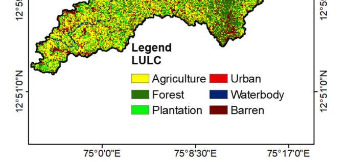
Water 2020, 12, 2400                                                                               6 of 25

2.2.1. Gauge-Based Meteorological Data
     Since the study area is poorly gauged, daily precipitation data for the period 1998–2013 were
collected from 0.25° × 0.25° grid points from the India Meteorological Department (IMD),
Government of India [39]. Similarly, daily maximum and minimum temperature, relative humidity,
wind speed, and solar radiation for the same period were obtained from the IMD (1° × 1°) [40] and
Climate Forecast System Reanalysis (CFSR, 0.25° × 0.25°) for calculating the potential
evapotranspiration (PET), which is required for the SWAT model. Even though CFSR data are not up
to the mark compared to, for example, ERA, in terms of resolution and near real-time availability,
ERA was proved to give poor streamflow simulation for Indian basins in the study by [41]. In
addition, studies have proved that CFSR data suit watershed modelling for meeting the challenges
of modelling ungauged watersheds and real-time hydrological modelling [42–44]. Hence, in the
present study, CFSR data were used for hydrological modelling. The daily discharge data for 2006–
2012 at Addoor gauging station were collected from the Central Water Commission (CWC) via the
India Water Resources Information System (IWRIS) platform.

2.2.2. TRMM Rainfall Data
     The Tropical Rainfall Measuring Mission (TRMM) Multi-Satellite Precipitation Analysis (TMPA)
3B42 version 7 algorithm (the post real-time version) is a gauge-adjusted product, superseding all the
previous versions of TRMM launched by the National Aeronautics and Space Administration NASA
and the Japanese Aerospace Exploration Agency (JAXA) in order to monitor precipitation in the
tropical and subtropical areas of 50° S–50° N with near-global coverage [45]. Its spatial and temporal
resolutions are 0.25° × 0.25° and 3-hourly, respectively, spanning from 1998 to the present. Daily
TRMM 3B42 v7 data is obtained by summing 3-hourly precipitation, which is obtained as a
combination of microwave, IR and gauge precipitation estimates from multiple independent
satellites. The daily rainfall data obtained from https://disc.gsfc.nasa.gov for the period 1998–2013
were used as input to drive the SWAT model.

2.2.3. CHIRPS Rainfall Data
      The CHIRPS rainfall dataset, Climate Hazards Group InfraRed Precipitation with Station data
version 2 (CHIRPS-2.0), is a 30+ year quasi-global rainfall dataset to analyse precipitation at different
scales. The CHIRPS was created in collaboration with scientists at the U.S. Geological Survey (USGS)
and Earth Resources Observation and Science (EROS) Center [11] to deliver reliable, up to date, and
more complete datasets for several early warning objectives. Spanning 50° S–50° N (and all
longitudes), starting from 1981 to present, CHIRPS incorporates 0.05° × 0.05° and 0.25° × 0.25°
resolution satellite imagery with in situ station data to create gridded rainfall time series for trend
analysis and seasonal drought monitoring. The CHIRPS is a gridded land-only precipitation dataset
developed by the synergistic use of satellite infrared cold cloud duration measurements and ground-
based rain gauge observations [11]. The daily rainfall data were extracted from
ftp://ftp.chg.ucsb.edu/pub/org/chg/products/CHIRPS-2.0/global_daily/netcdf/p25 for 1998–2013 as
an input for the rainfall runoff model. The main difference of climate hazard group climatology from
other precipitation climatology is that it uses long period satellite rainfall for deriving climatological
surfaces, which improves its performance in mountainous terrain [11].

2.3. Statistical Evaluation for the Satellite Precipitation Data
     In the present work, categorical and continuous statistics were executed between the satellite
precipitation data and the gauge-based products (IMD gridded data) to understand the error
characteristics and estimation capabilities of these data. The categorical statistics included Probability
of Detection (POD), False Alarm Ratio (FAR), and Critical Success Index/Threat score (CSI/TS)
metrics, whereas continuous statistical indices included Correlation Coefficient (r), Root Mean Square
Error (RMSE), and Percentage Bias (PBIAS). The categorical statistics are the number of rainfall events
detected or missed by the satellite rainfall data with respect to gauge data. The continuous statistics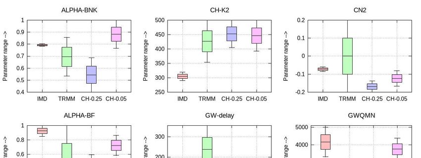
Water 2020, 12, 2400                                                                               7 of 25

signify efficiency of satellite datasets in estimating the amount of precipitation. The POD refers to the
ratio of hits (successful detection of rainfall as reference data) to the actual number of rainfall events
recorded according to base datasets (sum of hits and misses), whereas FAR represents the ratio of
false alarms (satellite precipitation products detecting the rainfall during non-occurrence of
precipitation in the base dataset) to the events that are not diagnosed by reference dataset [19,46]
      R represents the degree of significance or the synchronicity of precipitation differences between
satellite precipitation products and gauge or gridded data. The RMSE measures the precision of data
or the average error magnitude between the gauge and satellite data, while PBIAS shows the
likelihood of overestimation and underestimation. Lower bias and RMSE and higher R-value reflect
higher accuracy of satellite datasets with respect to reference datasets [47,48]. The POD and CSI/TS
values close to one, and FAR values close to zero reflect a satellite precipitation dataset’s capacity to
detect rainfall events.

2.4. Model Calibration, Validation, and Uncertainty Analysis
     The first five years (2001–2005) were used as a warm-up period to alleviate the initial conditions
in the model. The model was calibrated against the daily runoff during 2006–2009 and validated for
the period 2010–2012 for the Gurupura river. The calibration and validation of the model were
performed using Sequential Uncertainty Fitting version 2 (SUFI2) [49] in the SWAT Calibration and
Uncertainty Program (SWAT-CUP) tool developed for SWAT as an interface. The SUFI2 program
parameter uncertainty accounts for all the sources of uncertainties such as uncertainty in driving
variables (e.g., rainfall), conceptual model, parameters, and measured data. Initially, the models were
calibrated using the initial ranges of parameters listed in Table 2. According to the new parameters
suggested by the program [50] and their physical limitations, the ranges of each parameter are
modified after each iteration. The sensitivity analysis before calibration helps to reduce the number
of parameters and thereby reduce the computational time. Many iterations were carried out to obtain
an optimised parameter value. In each step, previous parameter ranges were updated to a new set of
value-based sensitivity matrix calculations. The parameters were then updated in such a way that the
new ranges were always smaller than the previous ranges and were centred around the best
simulation as per [50]. SUFI-2 methodology can be found elsewhere [51,52].

2.5. Performance Indices for Streamflow Simulation
     The ability of a hydrological model to reproduce observed streamflow could be expressed
through various output measurement indices. A variety of performance indices usually evaluate the
streamflow simulations. These evaluations include statistical performance measurements, e.g.,
Pearson’s correlation coefficient; weighted R2; hydrological performance measurements (e.g., Nash
and Sutcliffe Efficiency (NSE)). The performance evaluation of hydrological models is commonly
made by comparing the simulated and observed values. The statistical coefficients used for assessing
the model performance were the percent bias (PBIAS), coefficient of determination (R2), and the
Nash–Sutcliffe efficiency (NSE). The criteria suggested by [53] were used for evaluating the model
performance. The statistical indices were determined as follows:
     The percent bias (PBIAS) measures the tendency of the simulation compared to the observed
streamflow [33]. The optimal value of the percent bias is zero. A negative value indicates that the
model is overestimating, and a positive value indicates that the model is underestimating [54].
                                                         ∑       (       −       )
                                             =       ×                                                (1)
                                                             ∑       (       )
where O is the observed value, P is the predicted value, n is the number of samples, and            and
denote the average observed and predicted values, respectively.
The coefficient of determination (R2) is the proportion of the variation which can be explained by
fitting a regression line. It is a crucial output of regression analysis. The coefficient of determination
is a number that shows how well the data fit a statistical model. R2 is the squared value of the
correlation coefficient (r). Its value ranges from 0 to 1, higher values indicating lesser error variance.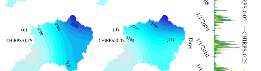
Water 2020, 12, 2400                                                                              8 of 25

                                              ∑       (       − )(       − )
                                     =
                                                                                                     (2)
                                          ∑       (       − ) ∑          (       − )

     The Nash–Sutcliffe Efficiency (NSE) is a statistical criteria used to assess the predictive power of
hydrological models. It is a normalised statistic that determines the relative magnitude of the residual
variance compared to the measured data variance [54].
                                                          ∑    (     −       )
                                              =       −                                              (3)
                                                          ∑    (     −       )
Water 2020, 12, 2400                                                                                                                                                     9 of 25

Table 2. The optimised value of each sensitive parameter for the four scenarios (“v_” and “r_” stand for replacement and a relative change to the initial parameter values,
respectively).

                                                                                             Lower   Upper                    Optimal Value
    Parameter                                     Description                                                                                                       Process
                                                                                             Limit   Limit       S1           S2        S3             S4
     r_CN2                                   Initial SCS CN II Value                         −0.20    0.20    −0.08(2)     0.18(7)      −0.18(1)     −0.12(4)       Runoff
 v_GW_DELAY                                 Groundwater delay (days)                          10      350      22.09(9)   309.25(8)     9.56(4)      14.61(3)    Groundwater
    v_CH_K2            Effective hydraulic conductivity in main channel alluvium (mm/h)        0      500     291.50(7)   483.44(5)    422.13(8)    487.19(9)      Channel
  v_Alpha_Bnk                     Baseflow alpha factor for bank storage [days]               0.5      1       0.79(1)     0.70(6)      0.54(9)       0.89(8)      Channel
  r_SOL_AWC                         Available water capacity of the soil layer                 0       1       0.31(3)     0.79(2)      0.24(2)       0.73(2)        Soil
 v_ALPHA_BF                                Base flow alpha factor (day)                        0       1       0.89(6)     0.42(9)      0.43(7)       0.86(5)    Groundwater
                       Threshold depth of water in the shallow aquifer required for return
   v_GWQMN                                                                                     0      5000    4100.8(8)   1391.14(4)   1706.12(6)   3742.63(7)   Groundwater
                                               flow to occur (mm)
    v_ESCO                           Soil evaporation compensation factors                    0        1       0.88(4)     0.45(3)      0.41(5)      0.36(6)     Evaporation
 v_GW_REVAP                             Groundwater “revap” coefficient                      0.02     0.2      0.17(5)     0.02(1)      0.11(3)      0.19(1)     Groundwater
      Note: Numbers in the parenthesis represent the rank of sensitive parameters.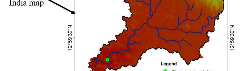
Water 2020, 12, 2400 10 of 25
2.6. Hydrological Signatures
The FDCs are the tools used for hydrological behaviour interpretation [55]. The FDCs are used
to systematically explain the frequency of high flows and low flows in the stream, and to determine
the probability of exceedance during the study duration. This provides both analytical and graphical
information to understand flow variability in the past and future. The SWAT model was run for all
four precipitation datasets, viz., IMD, TRMM, CHIRPS-0.25, and CHIRPS-0.05. Exceedance flow
analysis, performed by fitting an empirical equation [56] to the simulated flows at 5%, 10%, 25%, 50%,
and 70%, is identified. Q5 is the flow that exceeds 5% of the period of analysis, and Q10 is the flow
that exceeds 10% of the period of analysis, and so on. The flows corresponding to 5% and 10% are
indicative of the extreme flood events, 50% dependability indicates the median flow, 70% dependable
flow corresponds to the water availability for agriculture, and higher dependable flows correspond
the water availability for domestic requirements [57]. Since the study catchment experiences very
high flow during the monsoon season and negligible flows over the rest of the year, spatial variations
of above 30 percentile flow for the catchment are attempted. The simulated outflows obtained from
the SWAT model were further analysed to identify spatial heterogeneity at the subbasin scale for the
events and availability of water in the basin. The flow duration curve (FDC), a significant variability
signature, is the relationship between the discharge and the percentage of time that the discharge is
equalled or exceeded [28].
For simulating streamflow using the SWAT model, four calibration scenarios were considered
using gauge and satellite precipitation datasets.
Scenario 1 (S1): (a) the daily IMD rainfall data were first used to drive the model and optimise
the parameter values, (b) the daily TRMM, CHIRPS-0.25, and CHIRPS-0.05 rainfall data were
subsequently used to run the model with the same optimised parameter values, and (c) the simulated
runoffs for the three model runs were compared with IMD rainfall-driven results.
Scenario 2 (S2): the daily TRMM rainfall was used to drive the SWAT model and optimise the
parameter values, and then, the IMD, CHIRPS-0.25, and CHIRPS-0.05 rainfall were taken to drive the
model.
Scenario 3 (S3): CHIRPS-0.25 rainfall data were used to obtain the parameters, and the IMD,
TRMM, and CHIRPS-0.05 rainfall data were used to drive the model.
Scenario 4 (S4): CHIRPS-0.05 was used to run the model and obtained the optimal parameter
value, and the other three rainfall datasets viz. IMD, TRMM, and CHIRPS-0.25 were utilised to run
the model for comparison.
3. Results and Discussion
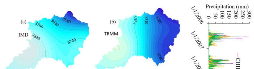
3.1. Spatial Distribution of Rainfall Data
Figure 3 represents the isohyetal maps for IMD, TRMM, CHIRPS-0.25, and CHIRPS-0.05 and
time series of daily rainfall data. The spatial distribution of annual average rainfall portrays
interesting characteristics of rainfall intensity in the windward side of the Western Ghats.
The catchment adjoining the Arabian Sea receives the highest annual rainfall (3700–3920 mm).
The midland of the catchment receives an annual average rainfall of 3400–3700 mm. This portion of
the catchment is characterised by agricultural and plantations. The upstream portion of the Gurupura
basin is dominated by the Western Ghats forest, having higher elevation that receives annual average
rainfall ranging from 3200 to 3400 mm. From Figure 3, it can be interpreted that all four datasets
exhibit a similar pattern of annual average rainfall over the catchment, with the highest amount of
rainfall at downstream followed by midland and minimum rainfall near the Ghats (Mountain
Ranges), whereas the TRMM projected less rainfall at high altitudes compared with others. This is
because TRMM uses passive microwave sensors of different wavelengths. Since these passive sensors
are not capable of detecting the orographic change in the liquid phase over the complex terrain [58],
the flow of the catchment in the mountainous area is underestimated. It could be observed that the
maximum annual average rainfall does not occur at the high altitude of the Western Ghats, which
may be due to the nonlinear temperature dependence of the saturation pressure. Similar findingsWater 2020, 12, 2400 11 of 25
were observed by [33], which indicated that the peak rainfall in the Western Ghats is 50 km away on
the windward side from the crest. From the time series plot of daily rainfall (Figure 3), it can be
observed that CHIRPS-0.25 and CHIRPS-0.05 precipitation products detect a higher amount of
rainfall during the monsoon season when compared with TRMM precipitation data. TRMM can
capture high flow during the monsoon season, whereas the CHIRPS precipitation product was able
to detect high flows for the rest of the year with respect to IMD precipitation data.
Figure 3. Spatial distribution and time series plot of (a) IMD (b) TRMM (c) CHIRPS-0.25 (d) CHIRPS-
0.05 rainfall datasets.
3.2. Categorical and Continuous Statistical Metrics
In the current study, three categorical statistical metrics (POD, FAR, and CSI/TS) were used to
understand the capability of satellite precipitation products to detect rainfall events (Table 3). The
TRMM exhibited a higher POD value (0.74) than CHIRPS-0.25 (0.71) and CHIRPS-0.05 (0.58). The
TRMM also exhibited a lower FAR value of 0.11 than CHIRPS-0.25 and CHIRPS-0.05 (0.18 and 0.16,
respectively). The FAR value near to zero represents the capability of a satellite rainfall product to
detect rainfall events accurately. The critical success index, which measures the satellite precipitation
products event that was correctly predicted, should have values closer to 1. CHIRPS-0.25 exhibited
an excellent value for CSI, which has better rainfall detection capabilities than TRMM.
Continuous statistics such as correlation coefficient (CC), bias, and root mean square error
(RMSE) were obtained for the satellite datasets with respect to IMD data. The correlation between
TRMM and IMD data was better than the correlation between CHIRPS and IMD data. Among the
satellite data, TRMM exhibited lower bias with IMD data, and a similar pattern was observed in the
case of RMSE also. From the overall statistical analysis of rainfall, TRMM produced better results
than CHIRPS-0.25 followed by CHIRPS 0.05.
Table 3. Categorical and continuous statistical values of precipitation datasets.Water 2020, 12, 2400 12 of 25
TRMM CHIRPS 0.25 CHIRPS 0.05
POD 0.74 0.71 0.58
FAR 0.11 0.18 0.16
CSI/TS 0.67 0.85 0.52
CC 0.56 0.47 0.47
Bias 0.91 1.02 1.02
RMSE 19.44 22.78 23.74
3.3. Evaluation of Streamflow Generation
As a large number of parameters are available, sensitive parameters are identified based on the
previous literature [59] and are used for calibration and validation of streamflow. The calibration of
the SWAT model was carried out by comparing the observed and simulated streamflow on a daily
scale at the outlet of the basin, i.e., Addoor. Around 14 parameters with varying ranges were used
for a different set of iterations required for different input product calibrations. The various
parameters used in the present study are CN2 (Initial SCS CN II Value), GW_Delay (Groundwater
delay (days)), CH_K2 (Effective hydraulic conductivity in main channel alluvium (mm/h)),
ALPHA_BNK (Baseflow alpha factor for bank storage (days)), SOL_AWC (Available water capacity
of the soil layer), Alpha_BF (Base flow alpha-factor (day)), GWQMN (Threshold depth of water in
the shallow aquifer required for return flow to occur (mm)), ESCO (Soil evaporation compensation
factors), GW_REVAP (Groundwater “revap” coefficient), CH_N2 (Manning ‘n’ coefficient for the
main channel), SOL_K (Saturated hydraulic conductivity of soil), REVAPMN (Depth of water
required for revap to occur in the shallow aquifer), SLSUBBSN (Average slope length), and SLSOIL
(Slope length for lateral subsurface flow). Out of the above parameters, a global sensitivity analysis
was performed using the SUFI-2 algorithm of SWAT-CUP and the nine most sensitive parameters
were selected for simulating the flow using the model. The allowable ranges and fitted values for
each dataset are represented in Table 2.
The daily simulation of streamflow using the four datasets is represented in Figure 4. It is noticed
that the IMD gridded data, which were derived from the observed gauged data, are the best at
simulating the observed flow compared with other datasets. At the daily time scale, the TRMM
underestimates the low flow, whereas it tries to match with the peak flow. This may be mainly
because of orographic precipitation during the monsoon season resulting due to the Western Ghats
mountainous region in the study area. The orographic lifting of moist air leads to cloud formation,
and even when the cloud top is relatively warm, rainfall will occur. The deep convection of this cloud
system is due to latent heat release. The infrared satellite sensors may not detect precipitation from
warm clouds and may lose the capture of ice loft, thereby detecting only a portion of rain from deep
convection [6,11,34,60]. This process may be the reason for the lower performance of the satellite data-
driven model than the IMD data-driven model. Even though the spatial resolution of both CHIRPS
datasets (0.25° and 0.05°) is different, it was found that the finer resolution does not make much
improvement in the flow simulation.Water 2020, 12, 2400 13 of 25
Figure 4. Daily simulation of streamflow for different precipitation datasets.
3.4. Hydrological Process Simulation
For the assessment of runoff predictions obtained from the IMD and satellite rainfall datasets, a
specific analysis was performed, applying the SWAT model with inputs from both datasets over the
Gurupura catchment. The SWAT model includes the parameters which need calibration for
reasonable simulation of the flow. Nonetheless, due to the correlation between model parameters
and the observed data, calibrated values were swayed [19]. The objective function for testing the
hydrological processes for four scenarios is the NSE. Each scenario is explained below to eliminate
the calibration effects of different datasets that are important [19] but not adequately discussed in the
relevant literature:
Scenario 1 (S1) was used to check the capacity of IMD gridded data and to assess the other
datasets in the simulation process. In the first phase of S1, the daily IMD rainfall data were used to
calibrate the model and to obtain the optimised value for each sensitive parameter. In the second
phase of S1, the daily TRMM, CHIRPS 0.25, and CHIRPS 0.05 rainfall data were used to drive the
model with the same optimised parameter values as phase S1. The rationale behind implementing
this second phase was to understand the effect of satellite precipitation products on the variations in
streamflow simulations under a set of standard calibration sensitive parameters [47]. The last phase
of S1 was to compare the simulated runoff of satellite datasets with the IMD rainfall-driven results.
In Scenarios 2, 3, and 4 (S2, S3, S4), the daily TRMM, CHIRPS 0.25, and CHIRPS 0.05 rainfall
were used to drive the SWAT model and optimise the parameter values, respectively. The
corresponding phases used in the case of S1 were performed. The rationale behind this scenario was
that (i) calibrating the model with different satellite precipitation products collected from various
sources reveals the impact of the rainfall data source on calibration performance and discharge
simulations and (ii) understanding the hydrological usability of these data products, which especially
helps in data-scarce and ungauged regions.
Based on the SUFI-2 algorithm of SWAT-CUP, sensitivity analysis was performed before
calibration for identifying the most sensitive parameters (Table 2). In general, in subtropical and
tropical regions, the SUFI-2 approach is a promising technique in calibration and uncertainty analysis
[61] and was adopted for the present study. It may be noted that each parameter exhibited different
optimised values for different scenarios. The curve number, which was the most sensitive parameter
among all, showed different optimised values for all the datasets. The values of CN2 for S1, S2, S3,
and S4 were −0.08, 0.18, −0.18, and −0.12, respectively. These values corresponded to the relative
values of the parameter in the SWAT model.
The shallow aquifer transit parameter GW_DELAY [62] showed a higher value of 309.25 days
for TRMM rainfall, whereas IMD and CHIRPS datasets had lower values. As the value was higher,
the lag between the entry of water to the shallow aquifer to release increased. Other groundwater
parameters, such as ALPHA_BF, which is a direct index for altering the recharge of groundwater
response, GWQMN—the measure of capillary rise, and GW_REVAP—the indicator of water
removed from the aquifer, corresponded to different optimised values for meeting up with the
observed streamflow.
It could be observed that the pairs of IMD and CHIRPS-0.05 and TRMM and CHIRPS-0.25
datasets represented an optimised value closer to each other for groundwater parameters. It may be
presumed that the spatial resolution in the CHIRPS datasets and their optimised parameter values
were significantly different, which showed a variation in resolution and parameter value.
The parameter ESCO is directly related to the evapotranspiration process [62]. As the value of
ESCO decreases, it makes the lower layer to compensate for the water deficit in the upper layer such
that the soil evapotranspiration increases. The satellite-based rainfall datasets depicted an opposite
trend to IMD, with a lower value of ESCO corresponding to higher soil evapotranspiration. Similar
patterns were expressed by the channel parameter CH_K2, which was used for estimating the peak
runoff. The sensitive parameter values of SOL_AWC, which influenced the streamflow and base flowWater 2020, 12, 2400 14 of 25
with a range of 0–1, are given in Table 2. As the value increased, the ability of soil to hold water also
increased, which led to decreased streamflow.
The details of model performance under all the four scenarios are presented in Table 4. In
Scenario 1, the model using IMD rainfall generated a strong overall fit for hydrological processes.
The NSE, PBIAS, and R2 for the Gurupura river using IMD data were 0.86, 0.87, 0.86 during
calibration and 0.76, −13.5, 0.81 for the validation period, respectively. This exhibited an excellent
performance rating as per [53], indicating that IMD rainfall data led to a robust and reliable testing
model for applicability and precision that could be used for validating and comparing the results
obtained from TRMM and CHIRPS rainfall (phase one in S1). Nevertheless, the subsequent
performances using TRMM and CHIPRS data exhibited relatively lower agreements (see phase two
above).Water 2020, 12, 2400 15 of 25
Table 4. Statistical indexes for Gurupura streamflow using different rainfall data.
IMD Rainfall Based TRMM Rainfall Based CHIRPS-0.25 Rainfall Based CHIRPS 0.05 Rainfall Based
Period of the Model
Scenario Model Model Model Model
Run
NSE PBIAS R2 NSE PBIAS R2 NSE PBIAS R2 NSE PBIAS R2
Calibration 0.86 0.87 0.86 0.66 −21.69 0.74 0.61 −7.21 0.61 0.65 −2.32 0.66
1
Validation 0.76 −13.50 0.81 0.70 −12.92 0.73 0.57 −7.03 0.57 0.63 0.44 0.64
Calibration 0.75 10.71 0.77 0.71 −14.98 0.75 0.55 4.90 0.56 0.54 −1.85 0.58
2
Validation 0.72 −5.52 0.73 0.71 −8.18 0.72 0.55 3.98 0.56 0.55 2.40 0.59
Calibration 0.73 2.08 0.73 0.63 −27.25 0.74 0.64 −6.20 0.65 0.63 −0.70 0.64
3
Validation 0.67 −13.19 0.70 0.67 −19.22 0.73 0.62 −7.41 0.63 0.61 1.66 0.62
Calibration 0.75 −0.91 0.75 0.60 −30.8 0.74 0.67 −9.67 0.65 0.66 −13.76 0.69
4
Validation 0.70 −16.09 0.65 0.66 −22.60 0.75 0.62 −10.71 0.65 0.65 −11.01 0.67
Note: Values in bold represent the statistical index values obtained when those particular sets of precipitation data were used for calibrating the model.Water 2020, 12, 2400 16 of 25
The NSE, R2, and PBIAS were in the range 0.57 to 0.7, 0.57 to 0.74, and −21.69 to 0.44, respectively,
which are in the range of satisfactory and good performance rating as per [53]. The TRMM results
showed better agreement compared to CHIPRS-0.05 spatial resolution, which was better than the
coarser-resolution product of CHIRPS with 0.25 spatial resolutions.
For scenario 2, the model performance using TRMM also produced a good score, with NSE,
PBIAS, and R2 of 0.71, −14.98, 0.75 and 0.71, −8.18, 0.72 during calibration and validation, respectively.
The performance of IMD data with the TRMM optimised parameter showed a higher value than the
parent model (TRMM model), which is interesting. The CHIRPS data under S2 were also in the
acceptable range. In the case of S3 and S4, it was found that, as spatial resolution increased, the
performance of the model improved. This indicates that the resolution of datasets also has a vital role
in model performance and hydrological processes.
It showed higher performance for the IMD gridded data, irrespective of the parameters of the
models which were used for calibrating. While comparing the performance of the model simulations,
the IMD rainfall with driven streamflow emerged as the best followed by the TRMM, CHIRPS 0.05,
and CHIRPS 0.25. Since the TRMM and CHIRPS rainfall-driven model results were in the acceptable
range, they could be utilised for similar catchments for analysing hydrological responses, since these
datasets are available free of cost with different spatial and temporal resolutions. This result and the
performance of satellite precipitation products are particularly desirable for data-scarce and
ungauged river basins. Since the performance of the satellite precipitation data-driven model reduced
while using the calibrated parameters of the other datasets, it may be suggested that each dataset
should be calibrated and validated separately. Such findings are consistent with the findings of
[21,47,63].
It is noteworthy that the parameters of a dataset that provided better results during calibration
of the model served similar or higher performance for the other datasets by transferring the same
parameters in the model. For example, the IMD rainfall-driven model outperformed both TRMM and
CHIRPS models which were forced with calibrated parameters using TRMM and CHIRPS. When
TRMM data was used to simulate using the calibrated parameters of the CHIRPS-0.05 model, it
yielded better or higher results than when forced with CHIRPS-0.05 parameters. It is, therefore,
inferred from these results that the parameters from a dataset that proves efficient when calibrated
could be transferred to calibrate the model with other datasets. Nonetheless, it is recommended to
apply satellite precipitation product-specific sensitive parameters for calibration, because this often
leads to substantially improved hydrological simulations compared to a model calibrated with other
sensitive parameters of the satellite dataset or gage dataset [47,64].
3.5. Uncertainty of Model Parameters
The hydrological models reproduced streamflow by adjusting relevant model parameters and
converged to different optimal intervals of calibrated parameters [17]. The distribution of the range
of the most sensitive parameters for the four rainfall datasets is illustrated in Figure 5. Typically, the
most sensitive parameter in the streamflow simulation was curve number CN2 [46]. A different set
of rainfall data produced different ranges of parameter values. Among these, the most apparent
difference was seen in the TRMM range of values. A wide range of values was obtained using TRMM
for each iteration, whereas IMD fell within a very short range. Groundwater parameters such as GW-
DELAY, GW-REVAP, GWQMN, and ALPHA-BF also portrayed different ranges of values for
different datasets. However, it was not possible to find a typical range of values since the models
tried to merge with the observed value. The channel parameters, such as CH-K2 and ALPHA-BNK,
also exhibited different patterns. In brief, it could be inferred that no consistent pattern exists to
correlate the parameter ranges and their uncertainty for the precipitation products used in this study.
Additionally, it is not possible to determine which dataset will have higher uncertainty for the
parameters. A similar approach of study and results were analysed by [17], and the variability in the
estimated parameter was basin-specific.Water 2020, 12, 2400 17 of 25
Figure 5. Distribution of the sensitive parameter values using four rainfall datasets.
To generate an accurate and reliable output, SWAT-CUP will adjust volumes of different
hydrological components during calibration. Hence, it is essential to select a proper hydrological
model for finding the effectiveness of a particular dataset. Even though all input datasets produced
reasonable outputs, the distribution of a single parameter for streamflow differed apparently.
The value of ESCO was very high for the IMD data, which resulted in low soil
evapotranspiration when compared with other data estimates. Similarly, the value for SOL_AWC
was very low for IMD, which meant that the soil would have less capacity to hold water, increasing
the streamflow. These will subsequently affect different management practices such as groundwater
and surface water management, conjunctive use of water, etc. Consequently, these uncertainties may
be a cause of concern in the right decision-making process for water management practices [65].
3.6. Distribution of Hydrological Signature over the Catchment
Figure 6 depicts the FDCs for all rainfall-driven models at the outlet of the Gurupura catchment.
It is observed that CHIRPS-0.05 follows the same pattern as that of the IMD. The minimum flow
required for water supply and irrigation projects corresponds to Q90. The TRMM portrays a shifted
pattern for high flows when compared with other datasets, whereas it overlaps with other flow
quantiles as it moves towards the low flow.Water 2020, 12, 2400 18 of 25
Figure 6. Daily flow duration curve for the Gurpura river at the Addoor station.
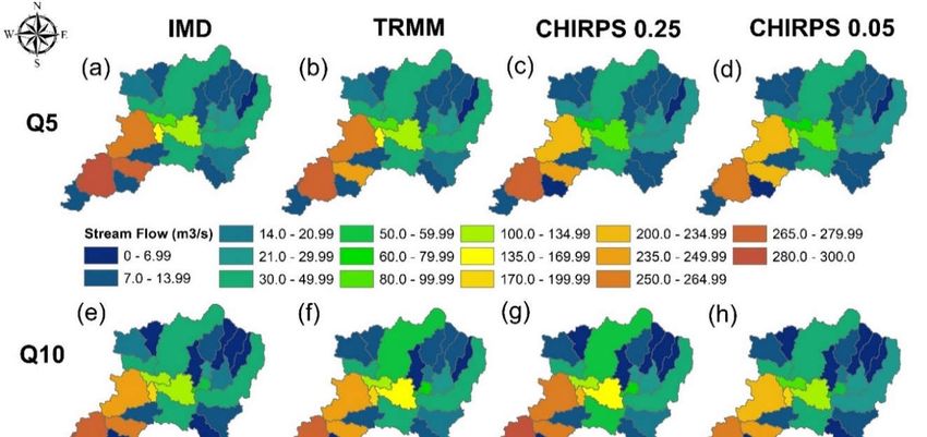
To perform a reliable flow analysis, dependable flow exceedances of Q5, Q10, Q25, Q50, and Q70
for the Gurupura catchment have been considered for all rainfall datasets. As the IMD gridded data
showed better results for the hydrological process, it could be considered as baseline data for testing
the capability of satellite datasets for illustrating the FDC spatially. Since the SWAT model was
calibrated for a subbasin over which the gauging station was present, it would likely simulate the
flow for all subbasins of the entire catchment. Applicability of the SWAT model to generate
streamflow for ungauged subcatchments was adopted here for deriving the hydrological signatures
spatially. Figure 7 illustrates the spatial variation of the dependable flow for the Gurupura catchment.
High flows depicting the extreme flood events are represented by Q5, Q10, and Q25 dependable flow.
The satellite datasets were capable of capturing these high flows for the catchment area. The TRMM
and CHIRPS indicated extreme events similar to the baseline established by the IMD data, which
indicates that these satellite data are useful for extreme event analysis. It is interesting to note that
the ability of TRMM data ceased for low flows when compared with CHIRPS data. Even though the
model performance of TRMM data superseded CHIRPS data, it failed to perform spatial dependable
flow analysis. Studies have reported that better statistical analysis for the precipitation data has not
yielded reliable hydrological analysis [19,25,26].Water 2020, 12, 2400 19 of 25
Figure 7. Spatial distribution of the dependable flow of (a) IMD-Q5, (b) TRMM-Q5, (c) CHIRPS 0.25-
Q5, (d) CHIRPS 0.05-Q5, (e) IMD-Q10, (f) TRMM-Q10, (g) CHIRPS 0.25-Q10, (h) CHIRPS 0.05-Q10,
(i) IMD-Q25, (j) TRMM-Q25, (k) CHIRPS 0.25-Q25, (l) CHIRPS 0.05-Q25, (m) IMD-Q50, (n) TRMM-
Q50, (o) CHIRPS 0.25-Q50, (p) CHIRPS 0.05-Q50, (q) IMD-Q70, (r) TRMM-Q70, (s) CHIRPS 0.25-Q70,
(t) CHIRPS 0.05-Q70, rainfall datasets for the Gurupura catchment.Water 2020, 12, 2400 20 of 25
The IMD and CHIRPS-0.25 data depicted the same kind of median flow (Q50) distribution,
whereas TRMM underestimated it at the mountainous region of the catchment. For estimating
agricultural water availability corresponding to Q70, CHIRPS-0.25 data were good since they exactly
corresponded to the IMD flow. The TRMM underestimated Q70 for more than half of the catchment,
indicating its weakness for producing this flow. It is to be noted that one cannot judge a dataset as
the best merely by just finding the performance indices. Further analysis has to be carried out for
finding the capability of data and its uses based on its application of the study [19,26]. For simulating
high flows, TRMM and CHIRPS may be used, whereas the TRMM is not suitable for low flow studies.
It also may be noted that the increased resolution of CHIRPS data did not improve the spatial
representation of flow quantile.
Connecting land use (Figure 2) and distribution of dependable flow, it was found that the TRMM
data underestimated the flow for the forested region of the catchment and at the places of high
altitude. This is because TRMM uses passive microwave sensors with multiple wavelengths. As these
passive sensors are not able to detect the orographic enhancement in the liquid phase over the
complex terrain [58], it underestimated flow at the mountainous region of the catchment. This
confirms the results reported earlier [66]. Since the catchment is dominated by agricultural land use,
the utmost care has to be taken while choosing the type of dataset for simulating Q70, which
corresponds to agricultural water availability. The majority of catchments in the coastal region of the
Western Ghats is agriculturally dominated. Hence, for analysing water availability for agricultural
purposes, it is recommended to choose IMD and CHIRPS-0.25 rainfall data over these regions. This
methodology could be applied for similar catchments elsewhere along the west coast of India. In
addition, TRMM overestimated the flow at the subbasin scale, which predominantly represents the
urban area. The land use land cover also affects satellite-based rainfall data for producing the
hydrological signature. Hence, the estimation of dependable flow and LULC will give a significant
linkage for the selection of satellite-based precipitation models. It is important to note that one should
be concerned not only with satellite-based precipitation but also with the selection of the hydrological
model [67].
Even if satellite-based precipitation is not capable of estimating the accurate amount of rainfall,
it could simulate accurate streamflow due to better calibration. Conversely, the precipitation dataset
which represents accurate rainfall may fail to generate proper streamflow due to poor selection of the
hydrological model. The results of this study, thus, would be helpful for users in the selection of
appropriate precipitation datasets based on their requirements.
4. Conclusions
The present work investigated the capability of four datasets of rainfall viz., IMD rainfall,
TRMM, CHIRPS-0.25, and CHIRPS-0.05 in simulating streamflow under different calibration
scenarios in a typical medium-sized catchment (Gurupura river) on the west coast of India. From
categorical and continuous statistical results, TRMM was able to detect better rainfall than CHIRPS
with respect to IMD rainfall data. All rainfall datasets were forced into the SWAT hydrological model
and calibrated separately to obtain the optimised parameters. The performance rating was found to
be in the following order as IMD, TRMM, CHIRPS-0.05, and CHIRPS-0.25. As the spatial resolution
of the CHIRPS dataset increased, the performance of the model to simulate the streamflow also
increased. The performance indicators R2, NSE, and PBIAS were in the ranges 0.63 to 0.86, 0.62 to
0.86, and −14.98 to 0.87, respectively, which showed that all datasets were in the acceptable range for
streamflow generation.
It could be inferred from the hydrological simulations that calibrated sensitive parameters of the
gauge or IMD dataset should not be used to calibrate the model with other satellite precipitation
products. Instead, each satellite dataset should be calibrated separately. The parameters of a best-
calibrated dataset should be transferred to calibrate other datasets. The optimised parameter values
for different rainfall datasets were different, with a varied range of parameter value distribution.Water 2020, 12, 2400 21 of 25
Even though the streamflow is adjusted to match the observed streamflow using the calibrated
parameters, other water balance components need to be accurate for adopting efficient water
management practices.
The potential of the SWAT model to produce streamflow for ungauged subcatchments was
evidenced by deriving the spatial hydrological signatures. The TRMM data underestimate the water
availability for agriculture purposes corresponding to Q70 dependable flow, whereas the CHIRPS
rainfall data are capable of capturing flow quantiles produced by the IMD gridded data. At the high
altitude and forest areas, TRMM underestimates rainfall and overestimates for the urban areas. The
CHIRPS-0.25 rainfall produces a similar pattern of flow quantiles of IMD than CHIRPS-0.05, which
conveys that the improvement in spatial resolution does not cause any significant improvement in
the flow quantiles, the key hydrological signature. Hence, it could be concluded that the uncertainties
in the model performance and parameters critically depend on the selection of precipitation datasets.
Different sets of data exhibit different results which may be a cause of concern while making
appropriate decisions related to water management practices. Hence, it is recommended to choose
appropriate rainfall data depending on the application. A similar strategy of calibration scenarios and
hydrological signatures in ungauged catchments may be used to interpret the effects of each dataset’s
sensitive parameters to understand catchment characteristics worldwide. The observations above
will help determine the most suitable dataset for hydrological application. In addition, the findings
in the study are useful for satellite-based rainfall developers to improve their products and provide
for users satellite rainfall-related applications.
Author Contributions: Investigation, T.M.S. and S.D.B.; Conceptualisation, T.M.S. and S.D.B.; Methodology,
T.M.S.; Writing—Original Draft, T.M.S.; Writing—Review and Editing, S.D.B., A.M., N.A.-A.; Funding
acquisition, N.A.-A.; Supervision, A.M. All authors have read and agreed to the published version of the
manuscript.
Funding: This research received no external funding.
Acknowledgments: The authors would like to extend their heartfelt gratitude to the Department of Water
Resources and Ocean Engineering of National Institute of Technology for providing valuable research data. We
are also thankful to all the institutes, organisations, and developers for providing the precipitation datasets.
Conflicts of Interest: The authors declare no conflict of interest.
References
1. Gao, F.; Zhang, Y.; Chen, Q.; Wang, P.; Yang, H.; Yao, Y. Comparison of two long-term and high-resolution
satellite precipitation datasets in Xinjiang, China. Atmos. Res. 2018, 212, 150–157,
doi:10.1016/j.atmosres.2018.05.016.
2. Stagl, J.; Mayr, E.; Koch, H.; Hattermann, F.F.; Huang, S. Effects of climate change on the hydrological cycle
in central and eastern Europe. In Managing Protected Areas in Central and Eastern Europe Under Climate
Change; Springer: Dordrecht, The Netherlands, 2014; pp. 31–43.
3. Chappell, A.; Renzullo, L.H.; Raupach, T.J.; Haylock, M. Evaluating geostatistical methods of blending
satellite and gauge data to estimate near real-time daily rainfall for Australia. J. Hydrol. 2013, 493, 105–114,
doi:10.1016/j.jhydrol.2013.04.024.
4. Su, Y.; Zhao, C.; Wang, Y.; Ma, Z. Spatiotemporal variations of precipitation in China using surface gauge
observations from 1961 to 2016. Atmosphere 2020, 11, 303, doi:10.3390/atmos11030303.
5. Zhao, C.; Garrett, T.J. Ground-based remote sensing of precipitation in the Arctic. J. Geophys. Res. Atmos.
2008, 113, 1–10, doi:10.1029/2007JD009222.
6. Ahmed, K.; Shahid, S.; Wang, X.; Nawaz, N. Evaluation of Gridded Precipitation Datasets over Arid
Regions of Pakistan. Water 2019, 11, 210, doi:10.3390/w11020210.
7. Chen, J.; Wang, Z.; Wu, X.; Chen, X.; Lai, C.; Zeng, Z.; Li, J. Accuracy evaluation of GPM multi-satellite
precipitation products in the hydrological application over alpine and gorge regions with sparse rain gauge
network. Hydrol. Res. 2019, 50, 1710–1729, doi:10.2166/nh.2019.133.
8. Tan, X.; Ma, Z.; He, K.; Han, X.; Ji, Q.; He, Y. Evaluations on gridded precipitation products spanning more
than half a century over the Tibetan Plateau and its surrounding. J. Hydrol. 2020,
doi:10.1016/j.jhydrol.2019.124455.You can also read